Search in book...
Toggle Font Controls
Create new playlist

Name your new playlist

Playlist description (optional)
Sign In

Email address

Password

Forgot Password?

or

Continue with Facebook

Continue with Google
Sign Up

Full Name

Email address

Confirm Email Address

Password

or

Continue with Facebook

Continue with Google

CHAPTER 20
CONSTRAINT EQUATIONS

20.1 INTRODUCTION

When doing an adjustment, it is sometimes necessary to fix an observation to a specific value. For instance, in Chapter 14, it was shown that the coordinates of a control station can be fixed by setting its dx and dy corrections to zero, and thus the corrections and their corresponding coefficients in the J matrix were removed from the solution. This is called a constrained adjustment. Another constrained adjustment occurs when the direction or length of a line is held to a specific value or when an elevation difference between two stations is fixed in differential leveling. In this chapter methods available for developing observational constraints are discussed. However, before discussing constraints, the procedure for including control station coordinates in an adjustment is described.

20.2 ADJUSTMENT OF CONTROL STATION COORDINATES

In examples in preceding chapters when the coordinates of a control station were excluded from the adjustments, hence their values held fixed, constrained adjustments were being performed. That is, the observations were being forced to fit the control coordinates. However, control is not perfect, and not all control is of equal reliability. This fact is evidenced by the fact that different orders of accuracy are used to classify control.

When more than minimal control is held fixed in an adjustment, the observations are forced to fit this control. For example, if the coordinates of two control stations are held fixed, but their actual positions are not in agreement with the values given by their held coordinates, the observations will be adjusted to match the erroneous coordinates. Simply stated, precise observations may be forced to fit less precise control. This was not a major problem in the days of transits and tapes, but does happen with modern instrumentation. This topic is discussed in more detail in Chapter 21.

To clarify the problem further, suppose that a new survey is tied to two existing control stations set from two previous surveys. Assume that the precision of the existing control stations is only 1:10,000. A new survey uses equipment and field procedures designed to produce a survey of 1:50,000. Thus, it will have a higher accuracy than either of the control stations to which it must fit. If both existing control stations are fixed in the adjustment, the new observations must distort to fit the errors of the existing control stations. After the adjustment, their residuals will show a lower-order fit that matches the control. In this case, it would be better to allow the control coordinates to adjust according to their assigned quality so that the observations are not distorted. However, it should be stated that the precision of the new coordinates relative to stations not in the adjustment can only be as good as the initial control.

The observation equations for control station coordinates are

(20.1) $images$

In Equation (20.1), x′ and y′ are the observed coordinate values of the control station, x and y the published coordinate values for the station, and v_x and v_y the residuals for the respective published coordinate values.

To allow the control to adjust, Equations (20.1) must be included in the adjustment for each control station. To fix a control station in this scheme, high weights are assigned to the station's coordinates. Conversely, low weights will allow a control station's coordinates to adjust. In this manner, all control stations are allowed to adjust in accordance with their expected levels of accuracy. In Chapter 21, it will be shown that when the control is included as observations, poor observations and control stations can be isolated in the adjustment by using weights.

EXAMPLE 20.1

A trilateration survey was completed for the network shown in Figure 20.1, and the following observations collected:

FIGURE 20.1 Trilateration network.

Control Stations
Station	X (ft)	Y (ft)
A	10,000.00	10,000.00
C	12,487.08	10,528.65

Distance Observations
From	To	Distance (ft)	σ (ft)	From	To	Distance (ft)	σ (ft)
A	B	1400.91	0.023	B	E	1644.29	0.023
A	E	1090.55	0.022	B	F	1217.54	0.022
B	C	1723.45	0.023	D	F	842.75	0.022
C	F	976.26	0.022	D	E	1044.99	0.022
C	D	1244.40	0.023	E	F	930.93	0.022

Perform a least squares adjustment of this survey, holding the control coordinates of stations A and C by appropriate weights (Assume that these control stations have a precision of 1:10,000).

SOLUTION

The first iteration linearized observation equations for the control coordinates of Equation (20.1) are

$images$

The J, X, and K matrices formed in this adjustment are

$images$

Notice that the last four rows of the J matrix correspond to linearized observation Equation (20.1) for the coordinates of control stations A and C. Each coordinate has a row with one in the column corresponding to its correction. Obviously, by including the control station coordinates, four unknowns have been added to the adjustment: dx_A, dy_A, dx_C, and dy_C. However, four observations have also been added. Therefore, the number of redundancies is unaffected by adding the coordinate observation equations. That is, the adjustment has the same number of redundancies with or without the control equations.

It is possible to weight a control station according to the precision of its coordinates. Unfortunately control stations are sometimes published with distance precisions rather than the covariance matrix elements that are required for weighting. However, estimates of the standard deviations of the coordinates can be computed from the published distance precisions. That is, if the distance precision between stations A and C is 1:10,000 or better, their coordinates should have estimated errors that yield a distance precision of 1:10,000 between the stations. To find the estimated errors in the coordinates that yield the appropriate distance precision between the stations, Equation (6.16) can be applied to the distance formula, resulting in

(20.2) $images$

In Equation (20.2), $images$ is the variance in distance D_ij and $images$ the variances in the coordinates of the end points of the line. Assuming that the estimated errors for the coordinates of Equation (20.2) are equal and substituting in the appropriate partial derivatives yields

(20.3) $images$

In Equation (20.3), σ_c is the standard deviation in the x and y coordinates. [Note that the partial derivatives appearing in Equation (20.3) were described in Section 14.2.] Factoring $images$ from Equation (20.3) yields

(20.4) $images$

where $images$ .

From the coordinates of A and C, distance AC is 2542.65 ft. To get a distance precision of 1:10,000, a maximum distance error of ±0.25 ft can exist. Assuming equal coordinate errors, then

$images$

Thus, σ_x = σ_y = ±0.18 ft. The computed standard deviations are used to weight the control in the adjustment. The weight matrix for this adjustment is

$images$

The adjustment results, obtained using the program ADJUST, are shown below.


****  Adjusted Distance Observations  ****
No. |  From  |   To   |  Distance  |  Residual  |
===========================================
   1|      A |      B |  1,400.910 |     -0.000 |
   2|      A |      E |  1,090.550 |     -0.000 |
   3|      B |      E |  1,644.288 |     -0.002 |
   4|      B |      F |  1,217.544 |      0.004 |
   5|      B |      C |  1,723.447 |     -0.003 |
   6|      C |      F |    976.263 |      0.003 |
   7|      C |      D |  1,244.397 |     -0.003 |
   8|      D |      E |  1,044.988 |     -0.002 |
   9|      E |      F |    930.933 |      0.003 |
  10|      D |      F |    842.753 |      0.003 |
===========================================

******  Adjusted Control Stations  ******
No. | Sta. |   Northing  |     Easting   |  N Res |  E Res |
=============================================================
   1|    C |  10,528.650 |    12,487.080 |  0.000 |  0.002 |
   2|    A |  10,000.000 |    10,000.000 | -0.000 | -0.002 |
=============================================================

Reference Standard Deviation = 0.25
Degrees of Freedom = 2

*******  Adjusted Unknowns  ******
Station|  Northing  |    Easting   | σ North| σ East | t ang° |A axis |B axis |
===============================================================================
      A|  10,000.000|     9,999.998|   0.033|   0.045| 168.000|  0.046|  0.033|
      B|  11,103.933|    10,862.483|   0.039|   0.034|  65.522|  0.040|  0.033|
      C|  10,528.650|    12,487.082|   0.033|   0.045| 168.000|  0.046|  0.033|
      D|   9,387.462|    11,990.882|   0.040|   0.038|  49.910|  0.044|  0.033|
      E|   9,461.900|    10,948.549|   0.039|   0.034| 110.409|  0.039|  0.033|
      F|  10,131.563|    11,595.223|   0.033|   0.034|  17.967|  0.034|  0.033|
===============================================================================

Notice that the control stations were adjusted slightly, as evidenced by their residuals. Also note the error ellipse data computed for each control station.

20.3 HOLDING CONTROL STATION COORDINATES AND DIRECTIONS OF LINES FIXED IN A TRILATERATION ADJUSTMENT

As demonstrated in Example 14.1, the coordinates of a control station are easily fixed during an adjustment. This is accomplished by assigning values of zero to the coefficients of the dx and dy correction terms. This method removes their corrections from the equations. In that particular example, each observation equation had only two unknowns, since one end of each observed distance was a control station that was held fixed during the adjustment. This was a special case of a method known as solution by elimination of constraints.

This method can be shown in matrix notation as

(20.5) $images$

(20.6) $images$

In Equation (20.6), A₁, A₂, X₁, X₂, L₁, and L₂ are the A, X, and L matrices partitioned by the constraint equations, as shown in Figure 20.2; C₁ and C₂ are the partitions of the matrix C consisting of the coefficients of the constraint equations; and V is the residual matrix. In this method, matrices A, C, and X are partitioned into two matrix equations that separate the constrained and unconstrained observations. Careful consideration should be given to the partition of C₁ since this matrix cannot be singular. If singularity exists, a new set of constraint equations that are mathematically independent must be determined. Also, since each constraint equation will remove one parameter from the adjustment, the number of constraints must not be so large that the remaining A₁ and X₁ have no independent equations or are themselves singular.

Geometrical depcition of A, X, and L matrices partitioned. — **FIGURE 20.2** A, X, and L matrices partitioned.

From Equation (20.6), solve for X₁ in terms of C₁, C₂, X₂, and L₂ as

(20.7) $images$

Substituting Equation (20.7) into Equation (20.5) yields

(20.8) $images$

Rearranging Equation (20.8), regrouping, and dropping V for the time being gives

(20.9) $images$

Letting A′ = −A₁C₁⁻¹C₂ + A₂, Equation (20.9) can be rewritten as

(20.10) $images$

Now Equation (20.10) can be solved for X₂, which, in turn, is substituted into Equation (20.7) to solve for X₁.

It can be seen that in the solution by elimination of constraint, the constraints equations are used to eliminate unknown parameters from the adjustment, thereby fixing certain geometric conditions during the adjustment. This method was used when the coordinates of the control stations were removed from the adjustments in previous chapters. In the following subsection, this method is used to hold the azimuth of a line during an adjustment.

20.3.1 Holding the Direction of a Line Fixed by Elimination of Constraints

Using this method constraint equations are written, and then substituted functionally into the observation equations to eliminate unknown parameters. To illustrate this, suppose that the direction of line IJ shown in Figure 20.3 is fixed. Thus, the position of J is constrained to move linearly along IJ during the adjustment. If J moves to J′ after adjustment then the relationship between the direction of IJ and dx_j and dy_j is

Geometrical depcition of Holding direction IJ fixed. — **FIGURE 20.3** Holding direction IJ fixed.

(20.11) $images$

For example, suppose that the direction of line AB in Figure 20.4 is to be held fixed during a trilateration adjustment. Noting that station A is to be held fixed and using prototype Equation (14.9), the following linearized observation equation results for observed distance AB.

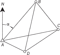
Geometrical depcition of Holding direction AB fixed in a trilateration adjustment. — **FIGURE 20.4** Holding direction AB fixed in a trilateration adjustment.

(20.12) $images$

Now, based on Equation (20.11), the following relationship is written for line AB:

(20.13) $images$

Substituting Equation (20.13) into Equation (20.12) yields

(20.14) $images$

Factoring dy_b in Equation (20.14), the constrained observation equation is

(20.15) $images$

Using this same method, the coefficients of dy_b for lines BC and BD are also determined resulting in the J matrix shown in Table 20.1.

TABLE 20.1 The J Matrix of Figure 20.3

	Unknowns
Distance	*dy_b*	*dx_c*	*dy_c*	*dx_d*	*dy_d*
AB	[(x_b − x_a)tan α + (y_b − y_a)]/AB	0	0	0	0
AC	0	(x_c − x_a)/AC	(y_c − y_a)/AC	0	0
AD	0	0	0	(x_d − x_a)/AD	(y_d − y_a)/AD
BC	[(x_b − x_c)tan α + (y_b − y_c)]/BC	(x_c − x_b)/BC	(y_c − y_b)/BC	0	0
BD	[(x_b − x_d)tan α + (y_b − y_d)]/BD	0	0	(x_d − x_b)/BD	(y_d − y_b)/BD
CD	0	(x_c − x_d)/CD	(y_c − y_d)/CD	(x_d − x_c)/CD	(y_d − y_c)/CD

For this example the K, X, and V matrices are

$images$

20.4 HELMERT'S METHOD

Another method of introducing constraints was originally presented by Friedrich R. Helmert in 1872. In this procedure, the constraint equation(s) border the reduced normal equations as

(20.16) $images$

To establish this matrix, the normal matrix and its matching constants matrix are formed, as has been done in Chapters 13 through 19. Following this, the observation equations for the constraints are formed. These observation equations are then included in the normal matrix as additional rows [C] and columns [C^T] in Equation (20.16) and their constants are added to the constants matrix as additional rows [L₂] in Equation (20.16). The inverse of this bordered normal matrix is computed. The matrix solution of the Equation (20.16) is

(20.17) $images$

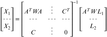
In Equation (20.17) X₂ is not used in the subsequent solution for the unknowns. This procedure is illustrated in the following examples. Both Example 20.2 and 20.3 are solved in the spreadsheet Chapter 18.xls, which is available on the book's companion website. In this spreadsheet, the examples are first solved using Helmert's method. Following this, they are solved using the elimination of constraints method. No matter the method used, the same results are always obtained.

EXAMPLE 20.2

A constrained differential leveling adjustment in figure 20.5, differential elevations were observed for a network where the elevation difference between stations B and E is to be held at −17.60 ft. The elevation of A is 1300.62 ft and the observed elevation differences for each line are shown below

FIGURE 20.5 Differential leveling network.

Line	From	To	Elevation (ft)	S (ft)
1	A	B	25.15	0.07
2	B	C	−10.57	0.05
3	C	D	−1.76	0.03
4	D	A	−12.65	0.08
5	C	E	−7.06	0.03
6	E	D	5.37	0.05
7	E	A	−7.47	0.05

Perform a least squares adjustment of this level net constraining the required elevation difference.

SOLUTION

The A, X, and L matrices are

$images$

The weight matrix (W) is

$images$

The reduced normal equations are

(a) $images$

The reduced normal matrix is now bordered by the constraint equation

$images$

which has a matrix form of

(b) $images$

The left-side of Equation (b) is now included as an additional row and column to the reduced normal matrix in Equation (a). The lower-right corner diagonal element of the newly bordered normal matrix is assigned a value of 0. Similarly, the right-hand side of Equation (b) is added as an additional row in the right-hand side of Equation (a). Thus, the bordered-normal equations are

Notice in Equation (c) that an additional unknown, X₂, is added at the bottom of the X to make the X matrix dimensionally consistent with the bordered-normal matrix of (c). Similarly, the right-hand side of the constraint Equation (b) is added to the bottom of the matrix. Using Equation (20.17), the resulting solution is

(d) $images$

From the X matrix in Equation (d), elevation of station B is 1325.686 and that for station E is 1308.086. Thus, the elevation difference between stations B and E is exactly −17.60, which was required by the constraint condition.

EXAMPLE 20.3

Constraining the azimuth of a line Helmert's method can also be used to constrain the direction of a line. In Figure 20.6 the bearing of line AB is to remain at its record value of N 0°04′ E. The data for this trilaterated network are:

FIGURE 20.6 Network for Example 20.3.

Control Stations			Station Initial Approximations
Station	X (m)	Y (m)	Station	X (m)	Y (m)
A	1000.000	1000.000	B	1003.07	3640.00
			C	2323.07	3638.46
			D	2496.08	1061.74

Distance Observations
From	To	Distance (m)	σ (m)	From	To	Distance (m)	σ (m)
A	C	2951.604	0.025	C	D	2582.534	0.024
A	B	2640.017	0.024	D	A	1497.360	0.021
B	C	1320.016	0.021	B	D	2979.325	0.025

Adjust this figure by the method of least squares holding the direction of the line AB using Helmert's method.

SOLUTION

Using procedures discussed in Chapter 14, the reduced normal equations for the trilaterated system are

(e) $images$

Following prototype Equation (15.9), the linearized equation for the azimuth of line AB is

(f) $images$

The observation equation for the constrained direction [Equation (f)] is then added to the border of the matrix of reduced normal Equations (e), which yields

(g) $images$

This is a nonlinear problem, and thus the solution must be iterated until convergence. The first two iterations yielded the X matrices listed as X₁ and X₂ below. The third iteration resulted in negligible corrections to the unknowns. The total of these corrections is shown as X_T below.

$images$

Adding the coordinate corrections of X_T to the initial approximations results in the final coordinates for stations B, C, and D of

$images$

Checking the solution: Using Equation (15.1), check to see that the direction of line AB was held to the value of the constraint.

$images$

20.5 REDUNDANCIES IN A CONSTRAINED ADJUSTMENT

The number of redundancies in an adjustment increases by one for each parameter that is removed by a constraint equation. An expression for determining the number of redundancies is

(20.18) $images$

where r is the number of redundancies in the system, m the number of observations in the system, n the number of unknown parameters in the system, and c the number of mathematically independent constraints applied to the system. In Example 20.2, there were seven observations in a differential leveling network that had four stations with unknown elevations. One constraint was added to the system of equations that fixed the elevation difference between B and E as −17.60. In this way, the elevation of B and E became mathematically dependent. By applying Equation (20.18), it can be seen that the number of redundancies in the system is r = 7 − 4 + 1 = 4. Without the aforementioned constraint, this adjustment would have only 7 − 4 = 3 redundancies. Thus, the constraint added one redundant observation to the adjustment while making the elevations of B and E mathematically dependent.

Care must be used when adding constraints to an adjustment. It would be possible to add as many mathematically independent constraint equations as there are unknown parameters. If that were done, all unknowns would be constrained or fixed, and it would be impossible to perform an adjustment. Furthermore, it is also possible to add constraints that are mathematically dependent equations. Under these circumstances, even if the system of equations has a solution, two mathematically dependent constraints would remove only one unknown parameter, and thus the redundancies in the system would increase by only one.

20.6 ENFORCING CONSTRAINTS THROUGH WEIGHTING

The methods described previously for handling constraint equations can often be avoided simply by overweighting the observations to be constrained in a weighted least squares adjustment. This was done in Example 16.2 to fix the direction of a line. As a further demonstration of the procedure of enforcing constraints by overweighting, Example 20.3 will be adjusted by writing observation equations for azimuth AB and the control station coordinates X_A and Y_A. These observations will be fixed by assigning a 0.001″ standard deviation to the azimuth of line AB and standard deviations of 0.001 ft to the coordinates of Station A.

The J, K, and W matrices for the first iteration of this problem are listed below. Note that the numbers have been rounded to three-decimal places for display purposes only.

$images$

The results of the adjustment (from the program ADJUST) are presented below.

*****************
Adjusted stations
*****************
Standard error ellipses computed
Station       X            Y         Sx        Sy        Su        Sv      t
=================================================================================
     A    1,000.000    1,000.000    0.0010    0.0010    0.0010    0.0010 135.00°
     B    1,003.072    3,640.003    0.0010    0.0217    0.0217    0.0010   0.07°
     C    2,323.081    3,638.468    0.0205    0.0248    0.0263    0.0186 152.10°
     D    2,496.081    1,061.748    0.0204    0.0275    0.0281    0.0196  16.37°

******************************
Adjusted Distance Observations
******************************
   Station   Station
  Occupied   Sighted       Distance          V          S
==========================================================
         A         C      2,951.620     0.0157     0.0215
         A         B      2,640.004    -0.0127     0.0217
         B         C      1,320.010    -0.0056     0.0205
         C         D      2,582.521    -0.0130     0.0215
         D         A      1,497.355    -0.0050     0.0206
         B         D      2,979.341     0.0159     0.0214

*****************************
Adjusted Azimuth Observations
*****************************
   Station   Station
  Occupied   Sighted          Azimuth       V        S′
===============================================================
         A         B       0° 04′ 00′     0.0′     0.0′

                    ****************************************
                             Adjustment Statistics 
                    **************************************** 
                             Iterations = 2
                           Redundancies = 1
                     Reference Variance = 1.499
                           Reference So = ±1.2 

               Passed X² test at 95.0% significance level!
                        X² lower value = 0.00
                        X² upper value = 5.02
               A priori value of 1 used for reference variance
                    in computations of statistics.
                          Convergence!

Notice in the previous adjustment that the control station coordinates remained fixed and the residual of the azimuth of line AB is zero. Thus, the azimuth of line AB was held fixed without the inclusion of any constraint equation. It was simply constrained by overweighting the observation. Also note that the final adjusted coordinates of stations B, C, and D match the solution in Example 20.3.

PROBLEMS

Note: For problems requiring least squares adjustment, if a computer program is not distinctly specified for use in the problem, it is expected that the least squares algorithm will be solved using the program MATRIX, which is available in the book's companion website. Partial answers to problems that are marked with an asterisk are provided in Appendix H.

*20.1 Given the following observed lengths in a trilateration survey, adjust the survey by least squares using the elimination of constraints method to hold the coordinates of A at x_a = 30,000.00 ft and y_a = 30,000.00 ft, and the azimuth of line AB to 2°31′56″± 3.0″ from North. Find the adjusted coordinates of B, C, and D.

Distance Observations
Course	Distance (ft)	S (ft)	Course	Distance (ft)	S (ft)
AB	9,813.20	0.033	BC	9,629.69	0.033
AC	13,764.18	0.044	BD	15,006.82	0.047
AD	11,395.99	0.037	CD	9,943.63	0.033

Initial Coordinates
Station	X (ft)	Y (ft)
B	30,433.56	39,803.63
C	40,054.84	39,399.65
D	41,386.93	29,545.64

20.2 Do Problem 20.1 using Helmert's method.
20.3 Do Problem 20.1 using the method of weighting for the azimuth.
20.4 Repeat Problem 20.1 using the following data.

Control Station Approximate Coordinates

Station X (m) Y (m) Station X (m) Y (m)

A 6509.325 6681.064 B 6402.643 7619.260

C 7329.700 7632.254

D 7427.389 6765.248

Distance Observations

Occupied Sighted Distance (m) S (m)

A B 944.243 0.005

A C 1256.093 0.006

A D 921.916 0.005

B C 927.136 0.005

B D 1333.965 0.006

C D 872.490 0.005

Azimuth Observation

Course Azimuth S

AB 353°30′46″ 3.2″
20.5 Do Problem 20.4 using Helmert's method.
20.6 Do Problem 20.4 using the method of weighting for the azimuth.
*20.7 Adjust the following differential leveling data using the elimination of constraints method. Hold the elevation of A to 136.485 m and the elevation difference ΔElev_BD to −3.750 m.

Elevation Differences

From To ΔElev (m) S (m)

A B −7.466 0.030

B C 4.101 0.030

D E 5.842 0.037

E A 5.368 0.042

C D −7.932 0.021
20.8 Repeat Problem 20.7 using Helmert's method.
20.9 Repeat Problem 20.7 using the weighting method.
20.10 Do Problem 13.14 holding distance BC to 100.00 ft.
1. *(a) Use the elimination of constraints method.
2. (b) Use Helmert's method.
3. (c) Compare the results of the adjustments from the different methods.
20.11 Do Problem 13.15 holding the elevation difference between V and Z to 30.00 ft.
1. (a) Use the elimination of constraints method.
2. (b) Use Helmert's method.
3. (c) Use the method of overweighting technique.
4. (d) Compare the results of the adjustments from the different methods.
20.12 Do Problem 12.15 holding the difference in elevation between Stations 2 and 8 to 5.500 m.
1. (a) Use the elimination of constraints method.
2. (b) Use Helmert's method.
3. (c) Use the method of overweighting technique.
*20.13 Assuming stations A and D are second-order, class I horizontal control (1:50,000), do Problem 14.9 by including the control in the adjustment.
20.14 Do Problem 15.8 assuming station A is first-order horizontal control (1:100,000) and D is second-order, class II horizontal control (1:20,000) using the method of weighting.
20.15 Do Problem 15.11 assuming the control stations A and B are first order control (1:100,000) and stations G and H are second-order, class II horizontal control (1:20,000) using the method of weighting.
20.16 Do Problem 16.16 assuming Stations A and D are third-order, class I control (1:10,000) using the method of weighting.

Control Station
A	6509.325	6681.064	B	6402.643	7619.260
			C	7329.700	7632.254
			D	7427.389	6765.248

Distance Observations
A	B	944.243	0.005
A	C	1256.093	0.006
A	D	921.916	0.005
B	C	927.136	0.005
B	D	1333.965	0.006
C	D	872.490	0.005

Azimuth Observation
Course	Azimuth	S
AB	353°30′46″	3.2″

Elevation Differences
A	B	−7.466	0.030
B	C	4.101	0.030
D	E	5.842	0.037
E	A	5.368	0.042
C	D	−7.932	0.021

PRACTICAL PROBLEMS

20.17 Develop a computational program that computes the coefficients for the J matrix in a trilateration adjustment with a constrained azimuth. Use the program to solve Problem 20.9.
20.18 Develop a computational program that computes a constrained least squares adjustment of a trilateration network using Helmert's method. Use this program to solve Problem 20.13.

..................Content has been hidden....................

You can't read the all page of ebook, please click here login for view all page.

Table of Contents for CHAPTER 20: CONSTRAINT EQUATIONS

Create new playlist

Sign In

Sign Up

20.1 INTRODUCTION

20.2 ADJUSTMENT OF CONTROL STATION COORDINATES

20.3 HOLDING CONTROL STATION COORDINATES AND DIRECTIONS OF LINES FIXED IN A TRILATERATION ADJUSTMENT

20.3.1 Holding the Direction of a Line Fixed by Elimination of Constraints

20.4 HELMERT'S METHOD

20.5 REDUNDANCIES IN A CONSTRAINED ADJUSTMENT

20.6 ENFORCING CONSTRAINTS THROUGH WEIGHTING

PROBLEMS

PRACTICAL PROBLEMS

Table of Contents for
CHAPTER 20: CONSTRAINT EQUATIONS