6.1 BASIC ERROR PROPAGATION EQUATION

As discussed in Section 1.2, unknown values are often determined indirectly by making direct measurements of other quantities that are functionally related to the desired unknown quantities. Examples in surveying include computing station coordinates from distance and angle observations, obtaining station elevations from rod readings in differential leveling, and determining the azimuth of a line from astronomical observations. As noted in Section 1.2, since all directly observed quantities contain errors, any values computed from them will also contain errors. This intrusion, or propagation, of errors that occurs in quantities computed from direct measurements is called error propagation. This topic is one of the most important discussed in this book.

In this chapter, it is assumed that all systematic errors and mistakes have been eliminated from a set of direct observations, so that only random errors remain. To derive the basic error propagation equation, consider the simple function, z = a₁x₁ + a₂x₂, where x₁ and x₂ are two independently observed quantities with standard errors σ₁ and σ₂, and a₁ and a₂ are constants. By analyzing how errors propagate in this function, a general expression can be developed for the propagation of random errors through any function.

Since x₁ and x₂ are two independently observed quantities, they each have different probability density functions. Let the errors in n determinations of x₁ be , and the errors in n determinations of x₂ be , then z_T, the true value of z for each independent observation, is

(6.1)

The values for z computed from the observations are

(6.2)

Substituting Equations (6.2) into Equations (6.1) and regrouping Equations (6.1) to isolate the errors for each computed value yields

(6.3)

From Equation (2.4) for the variance in a population, , and thus for the case under consideration, the sum of the squared errors for the value computed is

(6.4)

Expanding the terms in Equation (6.4) yields

(6.5)

Factoring terms in Equation (6.5) results in

(6.6)

Inserting summation symbols for the error terms in Equation (6.6) yields

(6.7)

Recognizing that the terms in parentheses in Equation (6.7) are by definition: , respectively, Equation (6.7) can be rewritten as

(6.8)

In Equation (6.8) the middle term, , is known as the covariance. This term shows the interdependence between the two unknown variables x₁ and x₂. As the covariance term decreases, the interdependence of the variables also decreases. When these terms are zero, the variables are said to be mathematical independent. Its importance in surveying is discussed in more detail in later chapters.

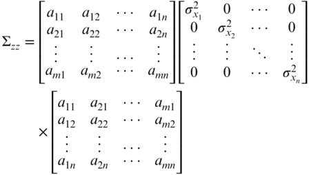
Equations (6.7) and (6.8) can be written in matrix form as

(6.9)

where Σ_zz is the variance-covariance matrix for the function z. It follows logically from this derivation that, in general, if z is a function of n independently measured quantities, x₁, x₂,…, x_n, then Σ_zz is

(6.10)

Further for a set of m functions with n independently measured quantities, x₁, x₂,…, x_n, Equation (6.10) expands to

(6.11)

Similarly, if the functions are nonlinear, a first order Taylor Series expansion can be used to linearize them.¹ Thus, a₁₁, a₁₂,…are replaced by the partial derivatives of the Z₁, Z₂,…with respect to the unknown parameters, x₁, x₂,…. Thus, after linearizing a set of nonlinear equations, the matrix for the function of Z can be written in linear form as

(6.12)

Equations (6.11) and (6.12) are known as the general law of propagation of variances (GLOPOV) for linear and nonlinear equations, respectively. Both Equations (6.11) and (6.12) can be written symbolically in matrix notation as

(6.13)

where Σ_zz is the covariance matrix for the function Z. For a nonlinear set of equations that is linearized using Taylor's Theorem, the coefficient matrix (A) is called a Jacobian matrix. That is, it is a matrix of partial derivatives with respect to the unknowns, as shown in Equation (6.12).

If the observations, x₁, x₂,…, x_n, are unrelated, that is, they are statistically independent, then the covariance terms are equal to zero and the right side of Equations (6.10) and (6.11) can be rewritten, respectively, as

(6.14)

(6.15)

If there is only one function Z, involving n unrelated quantities, x₁, x₂,…, x_n, then Equation (6.15) can be rewritten in algebraic form as

(6.16)

Equations (6.14) (6.15), and (6.16) express the special law of propagation of variances (SLOPOV). These equations govern the manner in which errors from statistically independent observations (i.e., ) propagate in a function. In these equations, individual terms represent the individual contributions to the total error that occur as the result of observational errors for each independent variable. When the size of a function's estimated error is too large, inspection of these individual terms will indicate the largest contributors to the error. The most efficient method to reduce the overall error in the function is to closely examine ways to reduce the largest individual error terms in Equation (6.16).

6.1.1 Generic Example

Let A = B + C, and assume that B and C are independently observed quantities. Note that and . Substituting these into Equation (6.16) yields

(6.17)

Using Equation (6.15) yields

Equation (6.17) yields the same results as Equation (6.16) after the square root of the single element is determined. In the equations above, standard error (σ) and standard deviation (S) can be used interchangeably.

6.2 FREQUENTLY ENCOUNTERED SPECIFIC FUNCTIONS

6.2.1 Standard Deviation of a Sum

Let A = B₁ + B₂ + ⋯ + B_n, where the B's are n independently observed quantities having standard deviations of , then by Equation (6.16),

(6.18)

6.2.2 Standard Deviation in a Series

Assume that the error for each observed value in Equation (6.18) is equal—that is, , then Equation (6.18) simplifies to

(6.19)

6.2.3 Standard Deviation of the Mean

Let be the mean obtained from n independently observed quantities y₁, y₂,…, y_n, each of which has the same standard deviation S. As given in Equation (2.1), the mean is expressed as

An equation for , the standard deviation of the mean is obtained by substituting the above expression into Equation (6.16). Since the partial derivatives of with respect to the observed quantities, y₁, y₂,…, y_n, is , the resulting error in is

(6.20)

Note that Equation (6.20) is the same as Equation (2.8).

6.3 NUMERICAL EXAMPLES

6.4 SOFTWARE

The computations in this chapter can be time-consuming and tedious often leading to computational errors in the results. It is often more efficient to program these equations in a computational package. The programming of the examples in this chapter is demonstrated in the Mathcad® electronic book on the companion website for this book. Figure 6.4 shows a partial listing of a Mathcad® worksheet used to solve Example 6.3. Notice that a function called radian was used to convert angles from sexagesimal units to radian units. After all of the variables for the problem are created, the problem is solved by creating an equation that looks very similar to those written in this book. The results of each expression are shown to the right of the equation. Oftentimes, the time that is spent learning a new programming language is more than rewarded in its efficient use to solve multiple problems. For example, the same worksheet can be used to solve problems that are similar to that in Example 6.3.

Another efficient method of programming these types of problems is to use a spreadsheet. In some spreadsheets, cells can be named, and thus equations can be entered using variables. For example, the expression for the , which is EC/A in Figure 6.5, was entered as AB/2*((−COS(A+B)*(SIN(B)*TAN(VA)+SIN(A)*TAN(VB)))/(SIN(A+B))^2 + (COS(A)*TAN(VB))/SIN(A+B)) where AB referred to the cell containing the distance AB, A the cell containing the angle A in radian units, B the cell containing the angle B in radian units, VA the cell containing the altitude angle v₁ in radian units, and VB the cell containing the altitude angle v₂ in radian units. Similarly, the other expressions were created using the named cells. While this method is not as clear as using a program such as Mathcad®, when an expression is entered carefully, the same results can be computed. Again, the resultant spreadsheet can be used to solve similar problems by simply change the data entry values.

6.5 CONCLUSIONS

Errors associated with any indirect measurement problem can be analyzed as described above. Besides being able to compute the estimated error in a function, the sizes of the individual errors contributing to the functional error can also be analyzed. This identifies those observations whose errors are most critical in reducing the functional error. An alternative use of the error propagation equation involves computing the error in a function of observed values prior to fieldwork. The calculation can be based on the geometry of the problem and the observations that are included in the function. The estimated errors in each observed value can be varied to correspond with those estimated using different combinations of available equipment and field procedures. The particular combination that produces the desired accuracy in the final computed function can then be adopted in the field. This analysis falls under the heading of survey planning and design. This topic is discussed further in Chapters 7, 19, and 21.

PROBLEMS

Note: Partial answers to problems marked with an asterisk can be found in Appendix H.

1. *6.1 In running a line of levels, 24 instrument setups are required, with a backsight and foresight taken from each. For each rod reading, the estimated error is ±1.5 mm. What is the error in the measured elevation difference between the origin and terminus?
2. 6.2 The estimated error in each angle of a 10-sided traverse is ±2.6″. What is the estimated error in the angular misclosure of the traverse?
3. 6.3 In Problem 2.10 compute the estimated error in the overall distance as measured by both the 100-ft and 200-ft tapes. Which tape produced the smallest estimated error?
4. 6.4 Determine the estimated error in length of AE that was observed in sections as follows:

   Section	Observed Length (m)	Standard Deviation (mm)
   AB	323.532	±3.2
   BC	465.083	±3.3
   CD	398.706	±3.2
   DE	120.683	±3.0

5. 6.5 A slope distance is observed as 2508.98 ± 0.013 ft. The zenith angle is observed as 98°05′26″ ± 4.3″. What are the horizontal distance and its estimated error?
6. 6.6 A slope distance is observed as 3581.98 ± 0.015 ft. The zenith angle is observed as 82°03′25″ ± 9.5″. What are the horizontal distance and its estimated error?
7. 6.7 A rectangular parcel has dimensions of 648.97 ± 0.018 ft by 853.03 ± 0.022 ft. What is the area of the parcel and the estimated error in this area?
8. 6.8 Same as Problem 6.7 except the dimensions are 536.792 ± 0.042 m by 600.087 ± 0.028 m.
9. *6.9 The volume of a cone is given by . A storage shed in the shape of a cone has a measured height of 30.0 ± 0.1 ft and radius of 30.0 ± 0.2 ft. What are the shed's volume and estimated error in this volume?
10. 6.10 Same as Problem 6.9, but the measured height is 15.00 ± 0.05 m and radius is 15.00 ± 0.08 m.
11. 6.11 Using an EDM instrument the rectangular dimensions of a large building 600.87 ± 0.019 ft by 350.08 ± 0.016 ft are laid out. Assuming only errors in distance observations, what are the
    1. (a) Area enclosed by the building and its standard deviation?
    2. (b) Perimeter of the building and its standard deviation?
12. 6.12 A particular total station's reading error is determined to be ±3.0″. After repeatedly pointing on a distant target with the same instrument, the observer determines an error due to both pointing and reading the circles of ±4.5″. What is the observer's pointing error?
13. *6.13 The dimensions of a storage shed under the rafters are 100.00 ± 0.03 ft long, 50 ± 0.02 ft wide, by 14.03 ± 0.02 ft high. What are the volume of this shed and the estimated error in this volume?
14. 6.14 Same as Problem 6.13 except the dimensions are 60.000 ± 0.003 m long, 40.000 ± 0.003 m wide, by 4.000 ± 0.003 m high.
15. 6.15 An EDM instrument manufacturer publishes its instrument's accuracy as ±(3 mm + 3 ppm). [Note: 3 ppm means 3 parts per million. This is a scaling error and is computed as (Distance × 3/1,000,000).]
    1. (a) What formula should be used to determine the error in a distance observed with this instrument?
    2. (b) What is the error in a 1256.78-ft distance measured with this EDM?
16. 6.16 Same as Problem 6.15 except the observed distance is 435.781 m.

    

17. 6.17 As shown in the accompanying sketch, a racetrack is measured in three simple components; a rectangle and two semicircles. Using an EDM with a manufacturer's specified accuracy of ±(3 mm + 3 ppm), the rectangle's dimensions measured at the inside of the track are 5280.00 ft by 850.00 ft. Assuming only errors in the distance observations, what are the
    1. (a) Standard deviations in each observation?
    2. (b) Length of the perimeter of the track?
    3. (c) Area enclosed by the track?
    4. (d) Standard deviation in the perimeter of the track?
    5. (e) Standard deviation in the area enclosed by the track?
18. 6.18 Repeat Problem 6.17, using the rectangle's dimensions as 1600.005 ± 0.006 m by 260.000 ± 0.003 m.
19. 6.19 The elevation of point C on the chimney shown in Figure 6.3 is desired. Field angles and distances are observed. Station A has an elevation of 345.36 ± 0.03 ft and Station B has an elevation of 353.86 ± 0.03. The instrument height, hi_A, at Station A is 5.53 ± 0.02 ft and the instrument height, hi_B, at Station B is 5.52 ± 0.02 ft. Zenith angles are read in the field. The other observations and their estimated errors are

    AB = 203.56 ± 0.02 ft

    What is the elevation of the stack and the standard deviation in this elevation?

20. 6.20 Same as Problem 6.19 with the following observations.

    ElevA = 248.35 ± 0.04 ft	ElevB = 242.87 ± 0.04 ft
    hiA = 5.53 ± 0.01 ft	hiB = 5.52 ± 0.01 ft

21. 6.21 Show that Equation (6.12) is equivalent to Equation (6.11) for linear equations.
22. 6.22 Derive an expression similar to Equation (6.9) for the function z = a₁x₁+ a₂x₂+ a₃x₃.

PRACTICAL EXERCISES

1. 6.23 With an engineer's scale, measure the radius of the circle in the accompanying sketch 10 times using different starting locations on the scale. Use a magnifying glass and interpolate the readings on the scale to a tenth of the smallest graduated reading on the scale.
   1. (a) What are the mean radius of the circle and its standard deviation?
   2. (b) Compute the area of the circle and its standard deviation.
   3. (c) Calibrate a planimeter by measuring a 2-in. square. Calculate the mean constant for the planimeter (k = units/4 in.²) and based on 10 measurements, determine the standard deviation in the constant.
   4. (d) Using the same planimeter, measure the area of the circle and determine its standard deviation.
2. 6.24 Develop a computational worksheet that solves Problem 6.19.