
CHAPTER 19
ERROR ELLIPSE
19.1 INTRODUCTION
![]() As discussed previously, after completing a least squares adjustment, the estimated standard deviations in the coordinates of an adjusted station can be calculated from covariance matrix elements. These standard deviations provide error estimates in the reference axes directions. In graphical representation, they are half the dimensions of a standard error rectangle centered on each station. The standard error rectangle has dimensions of 2Sx by 2Sy as illustrated for station B in Figure 19.1, but this is not a true representation of the error present at the station.
As discussed previously, after completing a least squares adjustment, the estimated standard deviations in the coordinates of an adjusted station can be calculated from covariance matrix elements. These standard deviations provide error estimates in the reference axes directions. In graphical representation, they are half the dimensions of a standard error rectangle centered on each station. The standard error rectangle has dimensions of 2Sx by 2Sy as illustrated for station B in Figure 19.1, but this is not a true representation of the error present at the station.

FIGURE 19.1 Standard error rectangle.
Simple deductive reasoning can be used to show the basic problem. Assume in Figure 19.1 that the XY coordinates of station A have been computed from the observations of distance AB and azimuth AzAB, which is approximately 30°. Further assume that the observed azimuth has no error at all, but that the distance has a large error, say ±2 ft. From Figure 19.1, it should then be readily apparent that the largest uncertainty in the station's position would not lie in either cardinal direction. That is, neither Sx nor Sy represents the largest positional uncertainty for the station. Rather, the largest uncertainty would be collinear with line AB and approximately equal to the estimated error in the distance. In fact, this is what happens.
In the usual case, the position of a station is uncertain in both direction and distance, and the estimated error of the adjusted station involves the errors of two jointly distributed variables, the x and y coordinates. Thus, the positional error at a station follows a bivariate normal distribution. The general shape of this distribution for a station is shown in Figure 19.2. In this figure, the three-dimensional surface plot [Figure 19.2(a)] of a bivariate normal distribution curve is shown along with its contour plot [Figure 19.2(b)]. Note that the ellipses shown in the xy plane of Figure 19.2(b) can be obtained by passing planes of varying levels through Figure 19.2(a) parallel to the xy plane. The volume of the region inside the intersection of any plane with the surface of Figure 19.2(a) represents the probability level of the ellipse. The orthogonal projection of the surface plot of Figure 19.2(a) onto the xz plane would give the normal distribution curve of the x coordinate, from which Sx is obtained. Likewise, its orthogonal projection onto the yz plane would give the normal distribution in the y coordinate from which Sy is obtained.

FIGURE 19.2 (a) Three-dimensional view and (b) contour plot of a bivariate distribution.
To fully describe the estimated error of a station, it is only necessary to show the orientation and lengths of the semiaxes of the error ellipse. A detailed diagram of an error ellipse is shown in Figure 19.3. In this figure, the standard error ellipse of a station is shown (i.e., one whose arcs are tangent to the sides of the standard error rectangle). The orientation of the ellipse depends on the t angle, which fixes the directions of the auxiliary, orthogonal uv axes along which the ellipse axes lie. The u axis defines the weakest direction in which the station's adjusted position is known. In other words, it lies in the direction of maximum estimated error in the station's coordinates. The v axis is orthogonal to u and defines the strongest direction in which the station's position is known, or the direction of minimum error. For any station, the value of t that orients the ellipse to provide these maximum and minimum values can be determined after the adjustment from the elements of the covariance matrix.

FIGURE 19.3 Standard error ellipse.
The exact probability level of the standard error ellipse is dependent on the number of degrees of freedom in the adjustment. This standard error ellipse can be modified in dimensions through the use of F critical values to represent an error probability at any selected percentage. It will be shown later that the percent probability within the boundary of standard error ellipse for a simple closed traverse is only 35%. Surveyors often use the 95% probability since this affords a higher level of confidence.
19.2 COMPUTATION OF ELLIPSE ORIENTATION AND SEMIAXES
As shown in Figure 19.4, the method for calculating the orientation angle t that yields maximum and minimum semiaxes involves a two-dimensional coordinate rotation. Notice that the t angle is defined as a clockwise angle from the y axis to the u axis. To propagate the errors in a point I from the xy system into an orthogonal uv system, the generalized law of the propagation of variances, discussed in Chapter 6, is used. The specific value for t that yields the maximum error along the u axis must be determined. The following steps accomplish this task.

FIGURE 19.4 Two-dimensional rotation.
- Step 1: Any point I in the uv system can be represented with respect to its XY coordinates as

Rewriting Equations (19.1) in matrix form yields

or, in simplified matrix notation,
- Step 2: Assume that for the adjustment problem in which I appears, there is a Qxx matrix for the xy coordinate system. The problem is to develop, from the Qxx matrix, a new covariance matrix Qzz for the uv coordinate system. This can be done using the generalized law for the propagation of variances, given in Chapter 6 as
(19.4)

where

Since ![]() is a scalar, it can temporarily be dropped and recalled again after the derivation. Thus,
is a scalar, it can temporarily be dropped and recalled again after the derivation. Thus,

where

- Step 3: Expanding Equation (19.5), the elements of the Qzz matrix are
- Step 4: The quu element of Equation (19.6) can be rewritten as

The following trigonometric identities are useful in developing the equation for t.
Substituting identity (a) into Equation (19.7) yields
Regrouping the first two terms and adding the necessary terms to Equation (19.8) to maintain equality yields

Substituting identity (c) and regrouping Equation (19.9) results in

Finally, substituting identity (b) into Equation (19.10) yields

To find the value of t that maximizes quu, differentiate quu in Equation (19.8) with respect to t and set the results equal to zero. This yields

Reducing Equation (19.12) yields
Finally, rearranging Equation (19.13) yields

Equation (19.14a) is used to compute 2t, and hence the desired angle t that yields the maximum value of quu. Note that the correct quadrant of 2t must be determined by noting the sign of the numerator and denominator in Equation (19.14a) before dividing by 2 to obtain t. Table 19.1 shows the proper quadrant for the different possible sign combinations of the numerator and denominator.
TABLE 19.1 Selection of the Proper Quadrant for 2ta
| Algebraic sign of sin 2t | cos 2t | Quadrant |
| + | + | 1 |
| + | − | 2 |
| − | − | 3 |
| − | + | 4 |
a When calculating for t, always remember to select the proper quadrant of 2t before dividing by 2.
Table 19.1 can be avoided by using the atan2 function available in most software packages. This function returns a value between −180° ≤ 2t ≤ 180°. If the value returned is negative, the correct value for 2t is obtained by adding 360°. The correct usage of the atan2 function in this instance is
The use of Equation (19.14b) is demonstrated in the Mathcad® worksheet c19.xmcd on the companion website.
Correlation between the latitude and departure of a station was discussed in Chapter 8. Similarly, the adjusted coordinates of a station are also correlated. Computing the value of t that yields the maximum and minimum values for the semiaxes is equivalent to rotating the covariance matrix until the off-diagonals are nonzero. Thus, the u and v coordinate values will be uncorrelated, which is equivalent to setting the ![]() element of Equation (19.6) equal to zero. Using the trigonometric identities previously noted, the element quv from Equation (19.6) can be written as
element of Equation (19.6) equal to zero. Using the trigonometric identities previously noted, the element quv from Equation (19.6) can be written as
Setting quv equal to zero and solving for t

Note that this yields the same result as Equation (19.14), which verifies the removal of the correlation.
- Step 5: In a fashion similar to that demonstrated in Step 4, the
 element of Equation (19.6) can be rewritten as
In summary, the t angle, semimajor axis (quu), and semiminor axis (![]() ) of the error ellipse are calculated using Equations (19.14), (19.7), and (19.17), respectively. These equations are repeated here, in order, for convenience. Note that these equations use only elements from the covariance matrix particular to the station, which will be demonstrated by example.
) of the error ellipse are calculated using Equations (19.14), (19.7), and (19.17), respectively. These equations are repeated here, in order, for convenience. Note that these equations use only elements from the covariance matrix particular to the station, which will be demonstrated by example.

Equation (19.18) gives the t angle that the u axis makes with the y axis. Equation (19.19) yields the numerical value for quu, which when multiplied by the reference variance ![]() gives the variance along the u axis. The square root of the variance is the semimajor axis of the standard error ellipse. Equation (19.20) yields the numerical value for qvv, which when multiplied by
gives the variance along the u axis. The square root of the variance is the semimajor axis of the standard error ellipse. Equation (19.20) yields the numerical value for qvv, which when multiplied by ![]() gives the variance along the v axis. The square root of this variance is the semiminor axis of the standard error ellipse. Thus, the semimajor and semiminor axes are
gives the variance along the v axis. The square root of this variance is the semiminor axis of the standard error ellipse. Thus, the semimajor and semiminor axes are
19.3 EXAMPLE PROBLEM OF STANDARD ERROR ELLIPSE CALCULATIONS
![]() In this section the error ellipse data for the trilateration example in Section 14.5 will be calculated. From the computer listing given for the solution of that problem, the following values are recalled:
In this section the error ellipse data for the trilateration example in Section 14.5 will be calculated. From the computer listing given for the solution of that problem, the following values are recalled:
- S0 = ± 0.136 ft
- The unknown X and covariance Qxx matrices were
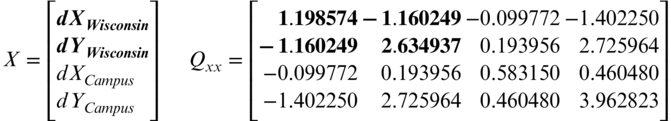
19.3.1 Error Ellipse for Station Wisconsin
Since the coordinates for station Wisconsin are in the first two rows of the X matrix only the corresponding 2 × 2 block diagonal elements of the Qxx matrix are used in the computations. From these elements, the tangent of 2t is
Notice that the sign of the numerator is negative and the denominator is positive. Thus, from Table 19.1 angle 2t is in the fourth quadrant, and 360° must be added to the computed angle. Hence,
and ![]()
Substituting the appropriate values into Equation (19.21), Su is

Similarly substituting the appropriate values into Equation (19.21), Sv is

The standard deviations in the coordinates, as computed by Equation (13.24), are

Since deriving the components of an error ellipse is an orthogonalization of the 2 × 2 block diagonal matrix for a station, this process can also be performed using eigenvectors and eigenvalues. This process is demonstrated in the Mathcad® worksheet C19.xmcd on the companion website. For example the eigenvalues of the 2 × 2 block diagonal matrix for station Wisconsin are 0.55222 and 3.28129, respectively. Thus, SU-WIS is ![]() and SV-WIS is
and SV-WIS is ![]() . Similarly, the eigenvector associated with the U axis can be used to compute the t angle. Using Station Wisconsin as an example, the eigenvector associated with the eigenvalue of 3.28129 is
. Similarly, the eigenvector associated with the U axis can be used to compute the t angle. Using Station Wisconsin as an example, the eigenvector associated with the eigenvalue of 3.28129 is ![]() . The t angle is computed as
. The t angle is computed as ![]() , which is the same value that was computed using Equation (19.18).
, which is the same value that was computed using Equation (19.18).
19.3.2 Error Ellipse for Station Campus
Using the same procedures as in Section 19.3.1, the error ellipse data for station Campus are
The 2 × 2 block diagonal submatrix is 

19.3.3 Drawing the Standard Error
To draw the error ellipses for stations Wisconsin and Campus of Figure 19.5, the error rectangle is first constructed by laying out the values of Sx and Sy using a convenient scale along the x and y axes, respectively. For this example, an ellipse scale of 4800 times the map scale was selected. The t angle is laid off clockwise from the positive y axis to construct the u axis. The v axis is drawn 90° counterclockwise from u to form a right-handed coordinate system. The values of Su and Sv are laid off along the U and V axes, respectively, to locate the semiaxis points. Finally, as shown in Figure 19.3, the ellipse is constructed so that it is tangent to the error rectangle and passes through its semiaxes points.

FIGURE 19.5 Graphical representation of error ellipses.
19.4 ANOTHER EXAMPLE PROBLEM
In this section, the standard error ellipse for station U in the example of Section 16.4 is calculated. For the adjustment, S0 = ± 1.82 ft, and the X and Qxx matrices are

Error ellipse calculations are

Notice in this example that the reference variance passed the χ2 test, and thus, the sample variance can be considered to be simply an estimate of the population variance, which has a value of 1. Thus, the population variance can be used to compute the semiaxes of the ellipse. This is done in the following computations:

Figure 19.6 shows the plotted standard error ellipse and its error rectangle.

FIGURE 19.6 Graphical representation of error ellipse.
19.5 THE ERROR ELLIPSE CONFIDENCE LEVEL
The calculations in Sections 19.3 and 19.4 produce standard error ellipses. These ellipses can be modified to produce error ellipses at any confidence level α by using an F statistic with two numerator degrees of freedom and the degrees of freedom for the adjustment in the denominator. Since the F statistic represents a ratio of two variances having different degrees of freedom, it can be expected that with increases in the number of degrees of freedom there will be corresponding increases in precision. The critical value for F(α,2,degrees of freedom) modifies the probability of the error ellipse for various confidence levels, as listed in Table 19.2. Notice that as the degrees of freedom increase, the F-statistic modifiers decrease rapidly and begin to stabilize for larger degrees of freedom. The confidence level of an error ellipse can be increased to any level by using the multiplier
Using the following equations, the percent probability for the semimajor and semiminor axes can be computed as

From the foregoing, it should be apparent that as the number of degrees of freedom (redundancies) increases, precision increases, and the size of error ellipse decreases. Using the techniques discussed in Chapter 4, the values listed in Table 19.2 are for the F distribution at 90% (α = 0.10), 95% (α = 0.05), and 99% (α = 0.01) probability. These probabilities are those most commonly used. Values from this table can be substituted into Equation (19.22) to determine the value of c for the probability selected and the given number of redundancies in the adjustment. This table is for convenience only and does not contain the values necessary for all situations that might arise.
TABLE 19.2 F(α,2,degrees of freedom) Statistics for Selected Probability Levels
| Probability | |||
| Degrees of Freedom | 90% | 95% | 99% |
| 1 | 49.50 | 199.50 | 4999.50 |
| 2 | 9.00 | 19.00 | 99.00 |
| 3 | 5.46 | 9.55 | 30.82 |
| 4 | 4.32 | 6.94 | 18.00 |
| 5 | 3.78 | 5.79 | 13.27 |
| 10 | 2.92 | 4.10 | 7.56 |
| 15 | 2.70 | 3.68 | 6.36 |
| 20 | 2.59 | 3.49 | 5.85 |
| 30 | 2.49 | 3.32 | 5.39 |
| 60 | 2.39 | 3.15 | 4.98 |
19.6 ERROR ELLIPSE ADVANTAGES
Besides providing critical information regarding the precision of an adjusted station position, a major advantage of error ellipses is that they offer a method of making a visual comparison of the relative precisions between any two stations. By viewing the shapes, sizes, and orientations of error ellipses, various surveys can be compared rapidly and meaningfully.
19.6.1 Survey Network Design
The sizes, shapes, and orientations of error ellipses are dependent on (1) the control used to constrain the adjustment, (2) the observational precisions, and (3) the geometry of the survey. The last two of these three elements are variables that can be altered in the design of a survey in order to produce optimal results. In designing surveys that involve the traditional observations of distances and angles, estimated precisions can be computed for observations made with differing combinations of equipment and field procedures. Also, trial variations in station placement, which creates the network geometry, can be made. Then these varying combinations of observations and geometry can be processed through least squares adjustments and the resulting station error ellipses computed, plotted, and checked against the desired results. Once acceptable goals are achieved in this process, the observational equipment, field procedures, and network geometry that provide these results can be adopted. This overall process is called network design. It enables surveyors to select the equipment and field techniques, and to decide on the number and locations of stations that provide the highest precision at lowest cost. This can be done in the office using simulation software before bidding the contract or entering the field.
In designing networks to be surveyed using the traditional observations of distance, angle, and directions, it is important to understand the relationships of those observations to the resulting positional uncertainties of the stations. The following relationships apply:
- Distance observations strengthen the positions of stations in directions collinear with the observed lines.
- Angle and direction observations strengthen the positions of stations in directions perpendicular to the lines of sight.
A simple analysis made with reference to Figure 19.1 should clarify the two relationships. Assume first that the length of line AB was precisely measured but its direction was not observed. Then the positional uncertainty of station B should be held within close tolerances by the observed distance, but it would only be held in the direction collinear with AB. The distance observation would do nothing to keep line AB from rotating, and in fact the position of B would be weak perpendicular to AB. On the other hand, if the direction of AB had been observed precisely but its length had not been measured, the positional strength of station B would be strongest in the direction perpendicular to AB. But an angle observation alone does nothing to fix distances between observed stations, and thus the position of station B would be weak along line AB. If both the length and direction AB were observed with equal precision, a positional uncertainty for station B that is more uniform in all directions would be expected. In a survey network that consists of many interconnected stations, analyzing the effects of observations is not quite as simple as was just demonstrated for the single line AB. Nevertheless, the two basic relationships stated still apply.
Uniform positional strength in all directions for all stations is the desired goal in survey network design. This would be achieved if, following least squares adjustment, all error ellipses were circular in shape and of equal size. Although this goal is seldom possible completely, by analyzing various combinations of geometric figures together with different combinations of observations and precisions diligently, this goal can be approached. Sometimes, however, other overriding factors, such as station accessibility, terrain, and vegetation preclude the actual use of an optimal design.
The network design process discussed above is aided significantly by the use of aerial photos and/or topographic maps. These products enable layout of trial station locations and permits analysis of the accessibility and intervisibility of these stations to be investigated. However, a field reconnaissance should be made before adopting a final design.
The global navigation satellite systems (GNSS) have brought about dramatic changes in all areas of surveying and network design is not an exception. Although GNSS does require overhead visibility at each receiver station for tracking satellites, problems of intervisibility between ground stations is eliminated. Thus, networks having uniform geometry can normally be laid out. Because each station in the network is occupied in a GNSS survey, the XYZ coordinates of the stations can be determined. This simplifies the problem of designing networks to attain error ellipses of uniform shapes and sizes. Additionally, recent photogrammetric images in the area of a project are often available over the Internet, which make checking satellite visibility problems possible. However, the geometric configuration of satellites plays a more important role in final station precisions. The positional dilution of precision (PDOP) can be a guide to the geometric strength of the observed satellites. In this case, the lower the PDOP, the stronger the satellite geometry. For more discussion on designing GNSS surveys, readers are referred to books devoted to the subject of GNSS surveying.
19.6.2 Example Network
Figure 19.7 shows error ellipses for two survey networks. Figure 19.7(a) illustrates the error ellipses from a trilateration survey with the nine stations, two of which (Red and Bug) were control stations. The survey includes 19 distance observations and 5 degrees of freedom. Figure 19.7(b) shows the error ellipses of the same network that was observed using triangulation and a baseline from stations Red to Bug. This survey includes 19 observed angles, and thus also has 5 degrees of freedom.

FIGURE 19.7 Network analysis using error ellipses: (a) trilateration for 19 distances; (b) triangulation for 19 angles.
With respect to these two figures, and keeping in mind that the smaller the ellipse, the higher the precision, the following general observations can be made:
- In both figures, stations Sand and Birch have the highest precisions. This, of course, is expected due to their proximity to control station Bug, and because of the density of observations made to these stations, which included direct measurements from both control stations.
- The large size of error ellipses at stations Beaver, Schutt, Bunker, and Bee of Figure 19.7(b) show that they have lower precision. This, too, is expected because there were fewer observations made to those stations. Also, neither Beaver nor Bee was connected directly by observations to either of the control stations.
- Stations White and Schutt of Figure 19.7(a) have relatively high East–West precisions and relatively low North–South precisions. Examination of the network geometry reveals that this could be expected. Distance measurements to those two points from station Red, plus an observed distance between White and Schutt, would have greatly improved the North–South precision.
- Stations Beaver and Bunker of Figure 19.7(a) have relatively low precisions East–West and relatively high precisions North–South. Again, this is expected when examining the network geometry.
- The smaller error ellipses of Figure 19.7(a) suggest that the trilateration survey will yield superior precision to the triangulation survey of Figure 19.7(b). This is expected since the distance measurements had a stated uncertainty of ±(5 mm + 5 ppm). In a 5000 ft distance, this yields an uncertainty of ±0.030 ft. To achieve the same precision, the comparable angle uncertainty would need to be

The proposed instrument and field procedures for the project that yielded the error ellipses of Figure 19.7(b) had an expected uncertainty of only ![]() . The ultimate design would include both observed distances and angles.
. The ultimate design would include both observed distances and angles.
These examples serve to illustrate the value of computing station error ellipses in an a priori analysis. The observations were easily and quickly made by a comparison of the ellipses in the two figures. Similar information would have been difficult, if not impossible, to determine from standard deviations. By varying the survey, it is possible ultimately to find a design that provides optimal results in terms of meeting a uniformly acceptable precision and survey economy.
19.7 OTHER MEASURES OF STATION UNCERTAINTY
Other measures of accuracies are sometimes called for in specifications. As discussed in Section 19.5, the standard error ellipse has a c-multiplier of 1.00 and a probability between 35% and 39%. Other common errors and probabilities are given in Table 19.3.
TABLE 19.3 Other Measures of Two-Dimensional Positional Uncertainties
| Probability (%) | C | Name |
| 35 – 39 | 1.00 | Standard error ellipse |
| 50.0 | 1.18 | Circular error probable (CEP) |
| 63.2 | 1.41 | Distance RMS (DRMS) |
| 86.5 | 2.00 | 2-sigma ellipse |
| 95.0 | 2.45 | 95% confidence level |
| 98.2 | 2.83 | 2DRMS |
| 98.9 | 3.00 | 3-sigma ellipse |
The orthogonalization of the submatrices demonstrated in Section 19.3.1 can be used to compute the error ellipsoids for three-dimensional coordinates from a GNSS adjustment or the three-dimensional geodetic network adjustment discussed in Chapter 23. That is, the uncertainties along the three orthogonal axes of the error ellipsoid can be computed using eigenvalues of the 3 × 3 block diagonal submatrix appropriate for each station. The common measures for ellipsoids are listed in Table 19.4.
TABLE 19.4 Measures of Three-Dimensional Positional Uncertainties
| Probability (%) | C | Name |
| 19.9 | 1.00 | Standard ellipsoid |
| 50.0 | 1.53 | Spherical error probable (SEP) |
| 61.0 | 1.73 | Mean radical spherical error (MRSE) |
| 73.8 | 2.00 | 2-sigma ellipsoid |
| 95.0 | 2.80 | 95% confidence level |
| 97.1 | 3.00 | 3-sigma ellipsoid |
The required accuracy for a control survey depends primarily on its purpose. Some major factors that affect accuracy are type and condition of equipment used, field procedures adopted, and the experience and capabilities of personnel employed. In 1998, the Federal Geographic Data Committee (FGDC) published detailed standards of accuracy and specifications for data disseminated by the federal government.2 The rationale for the standards was to provide a uniform set of standards specifying accuracies of various data capture methods for control surveys along with other analog and digital representations of survey data such as maps.
Table 19.5 lists the 1998 FGDC accuracy standards for control surveys. These standards are independent of the method of survey and based on a 95% confidence level. In order to meet these standards, control points in the survey must be consistent with all other points in the geodetic control network and not merely those within the particular survey. This is known as network accuracy and requires a comparison of survey results against network values or values captured using more accurate survey procedures. For example, the quality of a map can be determined by comparing at least 20 identifiable-point coordinate values against the locations of these same points as determined by an optical or GNSS survey.
TABLE 19.5 1998 FGDC Accuracy Standards: Horizontal, Ellipsoid Height, and Orthometric Height
| Accuracy Classifications | 95% Confidence Less Than or Equal To |
| 1 millimeters | 0.001 meters |
| 2 millimeters | 0.002 meters |
| 5 millimeters | 0.005 meters |
| 1 centimeters | 0.010 meters |
| 2 centimeters | 0.020 meters |
| 5 centimeters | 0.050 meters |
| 1 decimeters | 0.100 meters |
| 2 decimeters | 0.200 meters |
| 5 decimeters | 0.500 meters |
| 1 meters | 1.000 meters |
| 2 meters | 2.000 meters |
| 5 meters | 5.000 meters |
| 10 meters | 10.000 meters |
For horizontal surveys, the accuracy standard specifies the 95% radial error of the survey within which the true or theoretical location of the survey point falls 95% of the time. As shown in Figure 19.8, the 95% radial error is always shorter than the semimajor axes of the 95% error ellipse. To compute the probability of the radial error for a point, a constant C is determined using the semimajor (Su) and semiminor (![]() ) axes of the standard error ellipse from the least squares adjustment as
) axes of the standard error ellipse from the least squares adjustment as
Using a polynomial from Leenhouts (1985), the radial error of a point is approximated as
where r is the radial error for a station, Su the semimajor axis of the standard error ellipse, C as defined in Equation (19.24), and coefficients q0 through q3 are as listed in Table 19.6 for various probability levels. Thus, the 95% radial error for a station is computed as

FIGURE 19.8 A 95% circular error overlaying the 95% error ellipse for Station S.
TABLE 19.6 Coefficients for a Third-Order Polynomial Approximations of Radial Errors
| % Probability | q0 | q1 | q2 | q3 |
| 50 | 0.671956 | 0.011407 | 1.013704 | −0.523457 |
| 75 | 1.153896 | −0.121102 | 0.925793 | −2.198069 |
| 90 | 1.647743 | −0.62698 | 0.437189 | 0.127667 |
| 95 | 1.960790 | 0.004071 | 0.114276 | 0.371625 |
| 99 | 2.572111 | 0.127744 | −0.394634 | 0.727603 |
| 99.5 | 2.801799 | 0.165577 | −0.538393 | 0.821817 |
| 99.9 | 3.282670 | 0.228114 | −0.767617 | 0.964153 |
The vertical accuracy standard specifies a linear value (plus or minus) within which the true or theoretical location of the point falls 95% of the time. It is computed using the normal distribution multiplier of 1.9600 times the standard deviation for the elevation of the bench mark.
Procedures leading to classification of a survey to these standards involve four steps:
- The survey observations, field records, sketches, and other documentation are examined to ensure their compliance with specifications for the intended accuracy of the survey.
- A minimally constrained least squares adjustment of the survey observations is analyzed to guarantee that the observations are free from blunders and have been correctly weighted.
- The accuracy of control points in the local existing network to which the survey is tied is computed by random error propagation and weighted accordingly in the least squares adjustment of the survey network.
- The survey accuracy is checked at the 95% confidence level by comparing minimally constrained adjustment results against established control. The comparison takes into account the network accuracy of the existing control as well as systematic effects such as crustal motion or datum distortion.
Following the adjustment, a local accuracy for the survey can be determined using an average 95% radial error for the station coordinates or bench marks in the survey. The local accuracy represents the correctness of the coordinates of the stations relative to the coordinates of other stations in the survey. The network accuracy represents the correctness of the coordinates in the survey with respect to the geodetic datum. Thus, it is possible that a survey may have a very good local accuracy but not have a good network accuracy. To understand this, consider a survey for an engineering project that is based on a few local control stations in the project area. In order to qualify for determination of network accuracy, the survey should be connected to 20 or more control stations in the geodetic datum. Since this goes beyond the scope of the survey, which may be supporting a construction project, these standards also have guidelines for architectural, engineering, construction, and facilities management projects.
TABLE 19.7 Map Coordinates versus Surveyed Checkpoint Coordinates
| Map Coordinates | Surveyed Checkpoint Coordinates | Discrepancies/Residuals | |||||||
| Point | (1) x (m) | (2) y (m) | (3) z (m) | (4) X (m) | (5) Y (m) | (6) H (m) | (7) Δx | (8) Δy | (9) Δz |
| 1 | 326,064.94 | 27,695.00 | 604.22 | 326,069.477 | 27,700.068 | 594.056 | −4.537 | −5.068 | 10.164 |
| 2 | 332,436.19 | 27,596.91 | 578.46 | 332,438.494 | 27,605.343 | 587.351 | −2.304 | −8.433 | −8.891 |
| 3 | 329,244.19 | 25,219.12 | 585.16 | 329,235.172 | 25,217.616 | 583.693 | 9.018 | 1.504 | 1.467 |
| 4 | 326,054.07 | 22,891.32 | 558.35 | 326,059.779 | 22,890.734 | 563.272 | −5.709 | 0.586 | −4.922 |
| 5 | 332,431.37 | 22,795.94 | 571.03 | 332,437.285 | 22,796.579 | 575.159 | −5.915 | −0.639 | −4.129 |
| Number of Checkpoints | 5 | 5 | 5 | ||||||
| RMSE (m) | 5.91 | 7.76 | 6.72 | ||||||
| RMSEr | 7.41 | ||||||||
| 95% RMSE | 12.83 | 13.14 | |||||||
As stated previously, these standards can also be used to classify maps, scanning projects, and other data capture or representation processes. These standards closely align with the ASPRS Accuracy Standards for Digital Geospatial Data.3 The importance of classifying the accuracy of maps with statistical values is that all forms of maps, whether hardcopy or digital, can have their accuracy stated so that users understand the product and its potential uses. The root mean square error (RMSE) is defined as the square root of the average of squared discrepancies for points tested as discussed in Section 2.10. Discrepancies are the differences between coordinates and elevations of points taken from the map, and their values as determined by check surveys. Mathematically, it is denoted as

where n is the number of tested samples from the map, f(xi) is the position obtained from the map or geodetic datum, and xi is the position obtained from the check survey. For example, consider the data shown in Table 19.7. The map-derived values for coordinates of the points are shown in columns (1) – (3). The surveyed checkpoint coordinate values are shown in columns (4) – (6). The discrepancies shown in columns (7) – (9) are computed as the difference between the map and checkpoint coordinate values. Since the checkpoints must be surveyed at a higher accuracy than the map, these discrepancies can be thought of as residuals. Thus, the residual for the x coordinate of point 1 is computed as 326,064.94 – 32,069.477 = −4.537. Similarly, all other coordinate differences are determined. Using Equation (19.27), the RMSE in x (RMSEx), y (RMSEy), and z (RMSEz) are computed from their corresponding residuals as

From the RMSEx and RMSEy, a radial value for the horizontal positional accuracy can be determined as
To obtain the 95% positional horizontal accuracy for the map, the RMSEr is multiplied by 1.7308, which in this case results in a 95% positional horizontal accuracy of ±12.83 m for this map. To compute the 95% positional vertical accuracy for the map (RMSEz) is multiplied by 1.9600, which in this case yields ±13.17 m.
In order for RMSEs to be credible, the check survey must be performed at a higher level of accuracy than the map product. For example, assume a laser scanner is used to develop a map of a structure. In this instance, a conventional survey with a reflectorless total station will typically provide checkpoints at a higher level of accuracy and could be used to establish coordinates on clearly defined points, which are also visible and measured in the scan of the site. If a GNSS survey is to be used, special procedures as outlined in the NGS' Guidelines for Establishing GPS-Derived Ellipsoid Heights (Zilkoski, 1997) should be used to establish geodetic heights on clearly defined points. Additionally, the most recent geoid model must be applied to the geodetic heights to derive orthometric heights. However, if this method is used, realize that the geoid model for the area of interest may contain more error than is allowable. Alternately, a GNSS survey could be used to establish horizontal positioning while differential leveling or trigonometric leveling could be used to establish orthometric heights on points. It should also be recognized here that the network accuracy of a geodetic survey can be determined using this same method, with check coordinates coming from network stations.
PROBLEMS
Note: For problems below requiring least squares adjustment, if a computer program is not distinctly specified for use in the problem, it is expected that the least squares algorithm will be solved using the program MATRIX, which is included on the book's companion website. Partial answers are provided for problems marked with an asterisk in Appendix H.
- *19.1 Calculate the semiminor and semimajor axes of the standard error ellipse for the adjusted position of station U in the trilateration Example 15.1. Plot the figure using a scale of 1:10,000 and the error ellipse using an appropriate scale.
- 19.2 Calculate the semiminor and semimajor axes of the 95% confidence error ellipse for Problem 19.1. Plot this ellipse superimposed over the ellipse of Problem 19.1.
- 19.3 Repeat Problem 19.1 using the resection problem in Example 15.2.
- 19.4 Repeat Problem 19.2 using the data for Problem 19.3.
- 19.5 Same as Problem 19.1 except for the adjusted position of stations B and C of Example 15.3. Use a scale of 1:24,000 for the figure and plot the error ellipses using an appropriate multiplication factor.
Calculate the error ellipse data for the unknown stations in each problem.
- *19.6 Problem 14.1.
- 19.7 Problem 14.4.
- 19.8 Problem 14.8.
- 19.9 Problem 15.2.
- 19.10 Problem 15.5.
- 19.11 Problem 15.9.
- 19.12 Problem 16.1.
- 19.13 Problem 16.2.
- 19.14 Problem 16.3.
- 19.15 Problem 16.4.
- 19.16 Problem 16.5.
- 19.17 Problem 16.6.
- 19.18 Problem 16.7.
- 19.19 Problem 16.8.
- 19.20 Problem 16.9.
- 19.21 Problem 16.11.
Using a level of significance of 0.05, compute the 95% probable error ellipse for the stations in each problem.
- *19.22 Problem 19.12.
- 19.23 Problem 19.14.
- 19.24 Problem 19.17.
- 19.25 Problem 19.19.
- 19.26 Problem 19.20.
- 19.27 Using the program STATS, determine the percent probability of the standard error ellipse for a horizontal survey with
- *(a) 6 degrees of freedom.
- (b) 12 degrees of freedom.
- (c) 18 degrees of freedom.
- (d) 64 degrees of freedom.
- (e) 120 degrees of freedom.
PROGRAMMING PROBLEMS
- 19.28 Develop a computational program that takes the Qxx matrix and
 from a horizontal adjustment and computes error ellipse data for the unknown stations.
 - 19.29 Develop a computational program that solves Problems 19.15 and 19.16.