
CHAPTER 15
ADJUSTMENT OF HORIZONTAL SURVEYS: TRIANGULATION
15.1 INTRODUCTION
Prior to the development of electronic distance measuring equipment and the global navigation satellite systems, triangulation was the preferred method for extending horizontal control over long distances. The positions of widely spaced stations were computed from observed angles and a minimal number of observed distances called baselines. This method was used extensively by the National Geodetic Survey in extending much of the national network. Triangulation is still used by many surveyors in establishing horizontal control, although surveys that combine trilateration (distance observations) with triangulation (angle observations) are more common. In this chapter, methods are described for adjusting triangulation networks using least squares method.
A least squares triangulation adjustment can use condition equations or observation equations written either in terms of azimuths or angles. In this chapter the observation equation method is presented. The procedure involves a parametric adjustment where the parameters are coordinates in a plane rectangular system such as state plane coordinates. In the examples, the specific types of triangulations known as intersections, resections, and quadrilaterals will be adjusted.
15.2 AZIMUTH OBSERVATION EQUATION
![]() The azimuth equation in parametric form is
The azimuth equation in parametric form is
where ![]() , xi and yi are the coordinates of the occupied station I; xj and yj are the coordinates of the sighted station J; and C is a constant that depends on the quadrant in which point J lies as shown in Figure 15.1. From Figure 15.1, Table 15.1 can be constructed that relates the algebraic sign of the computed angle α in Equation (15.1) to the value of C and the value of the azimuth.
, xi and yi are the coordinates of the occupied station I; xj and yj are the coordinates of the sighted station J; and C is a constant that depends on the quadrant in which point J lies as shown in Figure 15.1. From Figure 15.1, Table 15.1 can be constructed that relates the algebraic sign of the computed angle α in Equation (15.1) to the value of C and the value of the azimuth.
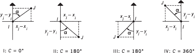
FIGURE 15.1 Relationship between the azimuth and the computed angle, α.
TABLE 15.1 Relationship between the Quadrant, C, and Azimuth
| Quadrant | Sign (xj − xi) | Sign (yj − yi ) | Sign α | C | Azimuth |
| I | + | + | + | 0 | α |
| II | + | − | − | 180° | α + 180° |
| III | − | − | + | 180° | α + 180° |
| IV | − | + | − | 360° | α + 360° |
15.2.1 Linearization of the Azimuth Observation Equation
Referring to Equation (15.1), the observation equation for an observed azimuth of line IJ is

where ![]() is the observed azimuth from station I to station
is the observed azimuth from station I to station ![]() ,
, ![]() the residual in the observed azimuth, xi and yi the most probable values for the coordinates of station I, xj, and yj the most probable values for the coordinates of station J, and C a constant with a value based on Table 15.1. Equation (15.2) is a nonlinear function involving variables xi, yi, xj, and yj, which can be rewritten as
the residual in the observed azimuth, xi and yi the most probable values for the coordinates of station I, xj, and yj the most probable values for the coordinates of station J, and C a constant with a value based on Table 15.1. Equation (15.2) is a nonlinear function involving variables xi, yi, xj, and yj, which can be rewritten as
where

As discussed in Section 11.10, nonlinear equations such as (15.3) can be linearized and solved using a first‐order Taylor series approximation. The linearized form of Equation (15.3) is

where ![]() ,
, ![]() ,
, ![]() , and
, and ![]() are the partial derivatives of F with respect to xi, yi, xj, and yj that are evaluated at the initial approximations and dxi, dyi, dxj, and dyj the corrections applied to the initial approximations after each iteration such that
are the partial derivatives of F with respect to xi, yi, xj, and yj that are evaluated at the initial approximations and dxi, dyi, dxj, and dyj the corrections applied to the initial approximations after each iteration such that
To determine the partial derivatives of Equation (15.4) requires the prototype equation for the derivative of tan−1(u) with respect to x, which is
Using Equation (15.6), the procedure for determining the ![]() is demonstrated as follows.
is demonstrated as follows.

By employing similar procedures, the remaining partial derivatives are

where ![]() .
.
If Equations (15.7) and (15.8) are substituted into Equation (15.4) and the results then substituted into Equation (15.3), the following prototype azimuth equation is obtained.

Both

are evaluated using the approximate coordinate values of the unknown parameters.
15.3 ANGLE OBSERVATION EQUATION
Figure 15.2 illustrates the geometry for an angle observation. In Figure 15.2, B is the backsight station, I the instrument station, and F the foresight station. As shown in the figure, an angle observation equation can be written as the difference between two azimuth observations, and thus for clockwise angles:


FIGURE 15.2 Relationship between an angle and two azimuths.
where θbif is the observed clockwise angle, ![]() the residual in the observed angle, xb and yb the most probable values for the coordinates of the backsight station B, xi and yi the most probable values for the coordinates of the instrument station I, xf and yf the most probable values for the coordinates of the foresighted station F, and D a constant that depends on the quadrants in which the backsight and foresight occur. This term can be computed as the difference between the C terms from Equation (15.1) as applied to the backsight and foresight azimuths; that is,
the residual in the observed angle, xb and yb the most probable values for the coordinates of the backsight station B, xi and yi the most probable values for the coordinates of the instrument station I, xf and yf the most probable values for the coordinates of the foresighted station F, and D a constant that depends on the quadrants in which the backsight and foresight occur. This term can be computed as the difference between the C terms from Equation (15.1) as applied to the backsight and foresight azimuths; that is,
Equation (15.10) is a nonlinear function of xb, yb, xi, yi, xf, and yf that can be rewritten as
where

Equation (15.11) expressed as a linearized, first‐order Taylor series expansion is

where ![]() ,
, ![]() ,
, ![]() ,
, ![]() ,
, ![]() , and
, and ![]() are the partial derivatives of F with respect to xb, yb, xi, yi, xf, and yf, respectively.
are the partial derivatives of F with respect to xb, yb, xi, yi, xf, and yf, respectively.
Evaluating partial derivatives of the function F and substituting into Equation (15.12), then substituting into Equation (15.11), results in the following equation.
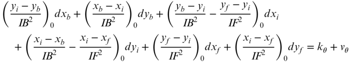
where

are evaluated at the approximate values for the unknown coordinates. Formulating the linearized angle observation equation can be thought of as the difference in two linearized azimuth equations. Using Equation (15.9) as a guide, the difference between the foresight and backsight azimuth is

Rearranging and regrouping Equation (a) yields Equation (15.13). This is left as an exercise for the reader.
In formulating the angle observation equation, remember that I is always assigned to the instrument station, B the backsight, and F the foresight station. This station designation must be strictly followed in employing prototype Equation (15.13) as will be demonstrated in the numerical examples that follow, and reproduced in the spreadsheet file Chapter 15.xls. As each is discussed, the reader may wish to refer to this file to see how the problem is implemented in a spreadsheet. Additionally, the file C15.xmcd demonstrates these examples in the higher‐level programming language of Mathcad. These files can be found on the companion website for this book.
15.4 ADJUSTMENT OF INTERSECTIONS
![]() When an unknown station is visible from two or more existing control stations, the angle intersection method is one of the simplest and sometimes most practical ways for determining the horizontal position of a station. For a unique computation, the method requires the observation of at least two horizontal angles from two control points. For example, angles θ1 and θ2 observed from control stations R and S in Figure 15.3 will enable a unique computation for the position of station U. If additional control is available, the computations for the unknown station's position can be strengthened by observing redundant angles such as angles θ3 and θ4 in Figure 15.3 and applying the method of least squares. In that case, for each of the four independent angles, a linearized observation equation is written in terms of the two unknown coordinates xu and yu.
When an unknown station is visible from two or more existing control stations, the angle intersection method is one of the simplest and sometimes most practical ways for determining the horizontal position of a station. For a unique computation, the method requires the observation of at least two horizontal angles from two control points. For example, angles θ1 and θ2 observed from control stations R and S in Figure 15.3 will enable a unique computation for the position of station U. If additional control is available, the computations for the unknown station's position can be strengthened by observing redundant angles such as angles θ3 and θ4 in Figure 15.3 and applying the method of least squares. In that case, for each of the four independent angles, a linearized observation equation is written in terms of the two unknown coordinates xu and yu.

FIGURE 15.3 Intersection example.
15.5 ADJUSTMENT OF RESECTIONS
![]() Resection is a method used for determining the unknown horizontal position of an occupied station by observing a minimum of two horizontal angles to a minimum of three stations whose horizontal coordinates are known. If more than three stations are available, redundant observations are obtained and the position of the unknown occupied station can be computed using the least squares method. Like intersection, resection is suitable for locating an occasional station and is especially well adapted over inaccessible terrain. This method is commonly used for orienting total station instruments in locations favorable for staking projects by radiation using coordinates.
Resection is a method used for determining the unknown horizontal position of an occupied station by observing a minimum of two horizontal angles to a minimum of three stations whose horizontal coordinates are known. If more than three stations are available, redundant observations are obtained and the position of the unknown occupied station can be computed using the least squares method. Like intersection, resection is suitable for locating an occasional station and is especially well adapted over inaccessible terrain. This method is commonly used for orienting total station instruments in locations favorable for staking projects by radiation using coordinates.
Consider the resection position computation for the occupied station U of Figure 15.4 having observed the three horizontal angles shown between stations P, Q, R, and S whose positions are known. To determine the position of station U, two angles could be observed. The third angle provides a check and allows a least squares solution for computing the coordinates of station U.

FIGURE 15.4 Resection example.
Using prototype Equation (15.13), a linearized observation equation can be written for each angle. In this problem, the vertex station is occupied and is the only unknown station. Thus, all coefficients in the Jacobian matrix follow the form used for the coefficients of dxi and dyi in prototype Equation (15.13). The method of least squares yields corrections, dxu and dyu, which gives the most probable coordinate values for station U.
15.5.1 Computing Initial Approximations in the Resection Problem
In Figure 15.4, only two angles are necessary to determine the coordinates of station U. Using stations P, Q, R, and U, a procedure to find the station U's approximate coordinate values is
- Step 1: Let
- Step 2: Using the sine law with triangle PQU,
and with triangle URQ,
- Step 3: Solving Equations (a) and (b) for QU and setting the resulting equations equal to each other yields
- Step 4: From Equation (c), let H be defined as
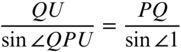
- Step 5: From Equation (15.16),
- Step 6: Solving Equation (15.17) for the sin ∠QPU, and substituting Equation (d) into the result yields
- Step 7: From trigonometry:


Applying this relationship to Equation (e),
- Step 8: Dividing Equation (g) by cos ∠URQ and rearranging yields
- Step 9: Solving Equation (h) for ∠URQ gives
- Step 10: From Figure 15.4,
- Step 11: Again applying the sine law yields
- Step 12: Finally, the initial coordinates for station U are
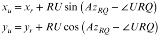 (15.21)


15.6 ADJUSTMENT OF TRIANGULATED QUADRILATERALS
![]() The quadrilateral is the basic figure for triangulation. Procedures like those used for adjusting intersections and resections are also used to adjust this figure. In fact, the parametric adjustment using the observation equation method can be applied to any triangulated geometric figure, regardless of its shape.
The quadrilateral is the basic figure for triangulation. Procedures like those used for adjusting intersections and resections are also used to adjust this figure. In fact, the parametric adjustment using the observation equation method can be applied to any triangulated geometric figure, regardless of its shape.
The procedure for adjusting a quadrilateral consists in first using a minimum number of the observed angles to solve triangles and computing initial values for the coordinates. Corrections to these initial coordinates are then calculated by applying the method of least squares. The procedure is iterated until the solution converges. This yields the most probable coordinate values. A statistical analysis of the results is then made. The following example illustrates the procedure.
PROBLEMS
Note: Partial answers to problems marked with an asterisk can be found in Appendix H.
- *15.1 Given the following observations and control station coordinates to accompany figure, what are the most probable coordinates for station E using an unweighted least squares adjustment?
Control Stations Station X (ft) Y (ft) A 10,000.00 10,000.00 B 11,498.58 10,065.32 C 12,432.17 11,346.19 D 11,490.57 12,468.51 Angle Observations Backsight (b) Occupied (i) Foresight (f) Angle S (″) E A B 90°59′57″ ±3.3 A B E 40°26′02″ ±3.7 E B C 88°08′55″ ±3.9 B C E 52°45′02″ ±3.7 E C D 51°09′55″ ±3.8 C D E 93°13′14″ ±4.0 
- 15.2 Repeat Problem 15.1 using a weighted least squares adjustment with weights of 1/S2 for each angle. What are the:
- (a) Most probable coordinates for station E and their standard deviations?
- (b) Reference standard deviation of unit weight?
- (c) Adjusted angles, their residuals, and standard deviations?
- 15.3 Given the following observations and control station coordinates to accompany Figure 15.3, what are the:
- (a) Most probable coordinates for station E and their standard deviations?
- (b) Reference standard deviation of unit weight?
- (c) Adjusted angles, their residuals, and standard deviations?
Control Stations Station Easting (m) Northing (m) R 6,735.656 6,061.097 S 6,894.607 5,517.132 T 6,693.269 4,920.183 Angle Observations Backsight (b) Occupied (i) Foresight (f) Angle S (″) U R S 49°07′42″ ±4.6 R S U 103°13′02″ ±4.9 U S T 111°42′34″ ±4.6 S T U 41°26′28″ ±4.3 - *15.4 Given the following observed angles and control coordinates for the resection problem of Figure 15.4.

Assuming equally weighted angles, what are the most probable coordinates for station U?
Control Stations Station X (ft) Y (ft) P 9000.00 9000.00 Q 9000.00 7500.00 R 9000.00 2500.00 S 9000.00 1200.00 - 15.5 If the estimated standard deviations for the angles in Problem 15.4 are S1 = ±4.5″, S2 = ±4.3″, and S3 = ±3.6″, what are the:
- (a) Most probable coordinates for station U and their standard deviations?
- *(b) Reference standard deviation of unit weight?
- (c) Adjusted angles, their residuals, and standard deviations?
- 15.6 Repeat Problem 15.5 using the following data.
Control Stations Station X (ft) Y (ft) P 8,593.99 8,170.60 Q 8,812.99 7,566.58 R 9,145.02 7,170.97 S 9,014.33 6,711.78 Angle Observations Backsight (b) Occupied (i) Foresight (f) Angle S (″) P U Q 22°52′35″ ±5.4 Q U R 20°49′45″ ±5.0 R U S 18°54′10″ ±6.2 - 15.7 Using approximate (x, y) coordinates for station E of (24,514.027, 23,409.472), and given the following control coordinates and observed angles for an intersection problem:
Control Stations Station X (m) Y (m) A 643.154 8,213.066 B 1,093.916 37,422.484 C 37,515.536 37,061.874 D 39,408.739 7,491.846 Angle Observations Backsight Occupied Foresight Angle S (″) E A D 33°32′48″ ±3.5 E B A 59°59′24″ ±3.5 E C B 46°57′58″ ±3.5 E D C 39°26′00″ ±3.5 What are the:
- (a) Most probable coordinates for station E and their standard deviations?
- (b) Reference standard deviation of unit weight?
- (c) Adjusted angles, their residuals, and standard deviations?
- 15.8 The following control station coordinates, observed angles and standard deviations apply to the quadrilateral in Figure 15.5.
Control Stations Initial Approximations Station X (ft) Y (ft) Station X (ft) Y (ft) A 1536.43 210.86 B 176.67 2801.09 D 3798.06 205.98 C 2355.54 2826.52 Angle Observations Backsight Occupied Foresight Angle S (″) B A C 45°24′8″ ±3.7 C A D 72°44′00″ ±3.7 C B D 36°17′38″ ±3.7 D B A 26°40′40″ ±3.6 D C A 46°13′13″ ±3.7 A C B 71°56′40″ ±3.7 A D B 35°30′04″ ±3.7 B D C 25°32′33″ ±3.6 Do a weighted adjustment using the standard deviations to calculate weights. What are the
- *(a) Most probable coordinates for stations B and C and their standard deviations?
- (b) Reference standard deviation of unit weight?
- (c) Adjusted angles, their residuals, and standard deviations?
- 15.9 For the accompanying figure and the following observations, perform a weighted least squares adjustment.
- (a) Station coordinates and standard deviations.
- (b) Angles, their residuals, and standard deviations.
Control Stations Initial Approximations Station X (m) Y (m) Station X (m) Y (m) A 600.544 966.236 C 3969.023 4112.018 B 1061.624 4043.173 D 3860.927 955.098 Angle Observations Backsight Occupied Foresight Angle S (″) B A C 38°26′08″ ±2.2 C A D 43°14′15″ ±2.1 C B D 49°09′52″ ±2.2 D B A 50°42′47″ ±2.2 D C A 44°59′51″ ±2.2 A C B 41°41′08″ ±2.2 B D C 44°09′07″ ±2.2 A D B 47°36′44″ ±2.2 
- 15.10 Do Problem 15.9 using the additional horizon closure angles listed below.
Backsight Occupied Foresight Angle S (″) D A B 278°19′38″ ±2.2 A B C 260°07′18″ ±2.2 B C D 273°19′38″ ±2.2 C D A 268°14′03″ ±2.2 - (a) Station coordinates and standard deviations.
- (b) Angles, their residuals, and standard deviations.
- (c) Compare and discuss any differences or similarities between these results and those obtained in Problem 15.9.
- 15.11 The following observations were obtained for a triangulation chain shown in the accompanying figure.
Control Stations Initial Approximations Station X (m) Y (m) Station X (m) Y (m) A 1718.871 632.095 C 1668.571 1310.429 B 2191.570 715.709 D 2139.109 1296.242 G 1590.370 2560.743 E 1617.479 1649.217 H 2076.006 2597.745 F 2028.688 1934.566 Angle Observations B I F Angle S (″) B I F Angle S (″) C A D 36°33′50″ ±4.1 D E C 47°20′12″ ±7.0 D A B 47°38′41″ ±5.1 F E D 68°50′37″ ±5.4 A B C 58°42′10″ ±5.2 D F C 39°48′02″ ±4.4 C B D 36°09′45″ ±4.5 C F E 25°15′23″ ±5.1 D C B 46°56′47″ ±5.2 H E F 29°26′35″ ±4.7 B C A 37°05′14″ ±4.1 G E H 27°30′09″ ±3.1 B D A 37°29′19″ ±4.5 E F G 89°45′54″ ±5.1 A D C 59°24′16″ ±5.2 G F H 39°04′24″ ±4.2 E C F 38°33′24″ ±6.8 H G F 59°21′56″ ±5.2 F C D 61°44′32″ ±5.4 F G E 33°17′14″ ±3.6 C D E 32°21′36″ ±5.5 F H E 21°43′05″ ±3.8 E D F 46°05′58″ ±4.7 E H G 59°50′37″ ±4.8 Use ADJUST to perform a weighted least squares adjustment. Tabulate the final adjusted
- (a) Station coordinates and their standard deviations.
- (b) Angles, their residuals, and standard deviations.

- 15.12 Add the following horizon closure angles to the data in Problem 15.11 and use the program ADJUST to perform the adjustment.
B I F Angle S (″) B A C 275°47′22″ ±5.6 A C E 175°40′06″ ±7.3 C E G 186°52′52″ ±6.9 E G H 267°20′44″ ±5.2 G H F 278°26′18″ ±5.6 H F D 166°06′12″ ±5.0 F D B 184°39′06″ ±5.3 D B A 265°07′57″ ±6.0 - (a) Station coordinates and their standard deviations.
- (b) Angles, their residuals, and standard deviations.
- (c) Compare and discuss any differences or similarities between these results and those obtained in Problem 15.11.
- 15.13 Using the control coordinates from Problem 14.3 and the following angle observations, compute the least squares solution and tabulate the final adjusted
- (a) Station coordinates and their standard deviations.
- (b) Angles, their residuals, and standard deviations.
Angle Observations Backsight Occupied Foresight Angle S (″) B A C 60°00′34″ ±3.3 C A D 59°59′23″ ±2.9 C B D 43°04′22″ ±2.8 C B A 79°07′27″ ±3.4 D C A 58°17′31″ ±2.9 A C B 40°51′51″ ±3.0 A D B 23°56′43″ ±2.7 B D C 37°46′19″ ±2.7 - 15.14 The following observations were obtained for a triangulation chain.
Control Stations Initial Approximations Station X (ft) Y (ft) Station X (ft) Y (ft) A 3,190.04 8,433.74 B 3,711.26 10,408.62 D 3,671.87 14,314.29 C 3,981.71 12,055.36 H 7,475.32 8,437.20 E 5,491.00 9,032.76 K 7,590.44 14,142.31 F 5,509.17 11,145.10 G 5,519.02 13,102.09 I 7,213.18 10,377.56 J 7,311.66 12,317.91 Angle Observations B I F Angle S (″) B I F Angle S (″) B A E 60°37′23″ ±1.7 J F I 57°17′59″ ±1.8 E B A 67°04′41″ ±1.7 I F E 66°14′38″ ±1.8 F B E 59°58′55″ ±1.7 E F B 67°13′52″ ±1.8 C B F 58°23′48″ ±1.9 A E B 52°17′56″ ±1.6 F C B 68°32′07″ ±2.0 B E F 52°47′11″ ±1.7 G C F 65°02′32″ ±1.9 F E I 51°31′17″ ±1.7 D C G 63°33′32″ ±1.8 I E H 51°41′29″ ±1.7 G D C 48°54′53″ ±1.7 H E A 148°42′06″ ±1.7 D G K 120°03′38″ ±1.7 E H I 65°35′58″ ±1.8 K G J 50°17′30″ ±1.7 H I E 59°42′34″ ±1.8 J G F 66°39′44″ ±1.8 E I F 62°14′01″ ±1.8 F G C 55°27′39″ ±1.8 F I J 68°39′25″ ±1.9 C G D 67°31′30″ ±1.8 I J F 54°02′38″ ±1.8 B F C 53°04′04″ ±1.9 F J G 56°40′36″ ±1.8 C F G 59°29′48″ ±1.9 G J K 75°03′42″ ±1.9 G F J 56°39′38″ ±1.8 J K G 54°38′50″ ±1.8 Use ADJUST to perform a weighted least squares adjustment. Tabulate the final adjusted
- (a) Station coordinates and their standard deviations.
- (b) Angles, their residuals, and standard deviations.
- 15.15 Add the following horizon closure angles to the data in Problem 15.14 and use the program ADJUST to perform the adjustment.
B I F Angle S (″) B I F Angle S (″) E A B 299°22′38″ ±1.7 G K J 305°21′11″ ±1.8 A B C 174°32′30″ ±2.0 K J I 174°13′19″ ±1.9 B C D 162°51′49″ ±1.9 J I H 169°24′02″ ±1.9 C D G 311°05′06″ ±1.7 I H E 294°24′00″ ±1.8 - (a) Station coordinates and their standard deviations.
- (b) Angles, their residuals, and standard deviations.
- (c) Compare the results of the adjustment with that of Problem 15.14.
Use the ADJUST software to do the following problems.
- 15.16 Problems 15.2.
- 15.17 Problems 15.4.
- 15.18 Problem 15.5.
- 15.19 Problems 15.6.
- 15.20 Problems 15.8.
- 15.21 Show that Equation (a) can be rearranged and regrouped to match Equation (15.13).
PROGRAMMING PROBLEMS
- 15.22 Write a computational program that computes the coefficients for prototype Equations (15.9) and (15.13), and their k values given the coordinates of the appropriate stations. Use this program to determine the matrix values necessary to do Problem 15.6.
- 15.23 Prepare a computational program that reads a file of station coordinates, observed angles, and their standard deviations and then
- (a) Writes the data to a file in a formatted fashion.
- (b) Computes the J, K, and W matrices.
- (c) Writes the matrices to a file that is compatible with the MATRIX program.
- (d) Test this program with Problem 15.6.
- 15.24 Write a computational program that reads a file containing the J, K, and W matrices and then
- (a) Writes these matrices in a formatted fashion.
- (b) Performs one iteration of either a weighted or unweighted least squares adjustment of Problem 15.6.
- (c) Writes the matrices used to compute the solution and the corrections to the station coordinates in a formatted fashion.
- 15.25 Write a computational program that reads a file of station coordinates, observed angles, and their standard deviations and then
- (a) Writes the data to a file in a formatted fashion.
- (b) Computes the J, K, and W matrices.
- (c) Performs either a relative or equal‐weight least squares adjustment of Problem 15.6.
- (d) Writes the matrices used to compute the solution, and tabulates the final adjusted station coordinates and their estimated errors, and the adjusted angles together with their residuals and their estimated errors.
- 15.26 Prepare a computational program that solves the resection problem. Use this program to compute the initial approximations for Problem 15.3.