
CHAPTER 18
COORDINATE TRANSFORMATIONS
18.1 INTRODUCTION
The transformation of points from one coordinate system to another is a common problem encountered in surveying and mapping. For instance, a surveyor who works initially in an assumed coordinate system on a project may find it necessary to transform the coordinates to the state plane coordinate system. In GNSS surveying and in photogrammetry, coordinate transformations are used extensively. Since the inception of the North American Datum of 1983 (NAD 83), many land surveyors, management agencies, state departments of transportation, and others struggled with the problem of converting their multitudes of stations defined in the 1927 datum (NAD 27) to the 1983 datum. Although several mathematical models have been developed to make these conversions, all involve some form of coordinate transformation. This chapter covers the introductory procedures of using least squares to compute several well-known and often used transformations. More rigorous procedures, which employ the general least squares procedure, are given in Chapter 22.
18.2 THE TWO-DIMENSIONAL CONFORMAL COORDINATE
![]() The two-dimensional conformal coordinate transformation, also known as the four-parameter similarity transformation, has the characteristic that true shape is retained after transformation. It is used typically in surveying when converting separate surveys into a common reference coordinate system. An example of this is the procedure used by several commercial software packages to convert satellite-derived coordinates into a local reference frame. For example, this procedure can be used to convert GNSS-derived WGS 84 coordinates into one of the realizations in the NAD 83 coordinate system. This process, known as localization, is discussed further in Section 24.5. The two-dimensional conformal coordinate transformation can be thought of as a three-step process:
The two-dimensional conformal coordinate transformation, also known as the four-parameter similarity transformation, has the characteristic that true shape is retained after transformation. It is used typically in surveying when converting separate surveys into a common reference coordinate system. An example of this is the procedure used by several commercial software packages to convert satellite-derived coordinates into a local reference frame. For example, this procedure can be used to convert GNSS-derived WGS 84 coordinates into one of the realizations in the NAD 83 coordinate system. This process, known as localization, is discussed further in Section 24.5. The two-dimensional conformal coordinate transformation can be thought of as a three-step process:
- Scaling to create equal dimensions in the two coordinate systems.
- Rotation to make the reference axes of the two systems parallel.
- Translations to create a common origin for the two coordinate systems.
The scaling and rotation are each defined by one parameter. The translations involve two parameters. Thus, there are a total of four parameters in this transformation. The transformation requires a minimum of two points, called control points, which are common to both systems. With the minimum of two points, the four parameters of the transformation can be determined uniquely. If more than two control points are available, a least squares adjustment is possible. After determining values for the transformation parameters, any points in the original system can be transformed into the second system.
18.3 EQUATION DEVELOPMENT
Figure 18.1(a) and (b) illustrates two independent coordinate systems. In these systems, three common control points, A, B, and C exist (i.e., their coordinates are known in both systems). Points 1 through 4 have coordinates known only in the xy system of Figure 18.1(b). The problem is to determine XY coordinates in the system of Figure 18.1(a). The necessary equations are developed as follows:

FIGURE 18.1 Superimposed coordinate systems.
- Step 1: Scaling. To make line lengths as defined by the xy coordinate system equal to their lengths in the XY system, it is necessary to multiply xy coordinates by a scale factor, S. Thus, the scaled coordinates x′ and y′ are
- Step 2: Rotation. In Figure 18.2, the XY coordinate system has been superimposed on the scaled x′y′ system. The rotation angle, θ, is shown between the y′ and Y axes. To analyze the effects of this rotation, an X′Y′ system is constructed parallel to the XY system such that its origin is common with that of the x′y′ system. Expressions that give the (X′, Y′) rotated coordinates for any point (such as point 4 shown) in terms of its x′y′ coordinates are

FIGURE 18.2 Two-dimensional coordinate systems.
- Step 3: Translation. To finally arrive at XY coordinates for a point, it is necessary to translate the origin of the X′Y′ system to the origin of the XY system. Referring to Figure 18.2, it can be seen that this translation is accomplished by adding translation factors as follows:


If Equations (18.1) (18.2), and (18.3) are combined, a single set of equations results that transform the points of Figure 18.1(b) directly into Figure 18.1(a) as

Now letting S cos θ = a, S sin θ = b, TX = c, and TY = d and adding residuals to make redundant equations consistent, the resulting equation can be written as

18.4 APPLICATION OF LEAST SQUARES
Equations (18.5) represent the basic observation equations for a two-dimensional conformal coordinate transformation that have four unknowns: a, b, c, and d. The four unknowns embody the transformation parameters S, θ, TX, and TY. Since two equations can be written for every control point, only two control points are needed for a unique solution. When more than two are present, a redundant system exists for which a least squares solution can be found. As an example, consider the equations that could be written for the situation illustrated in Figure 18.1. There are three control points, A, B, and C, and thus the following six equations can be written

Equations (18.6) can be expressed in matrix form as
where
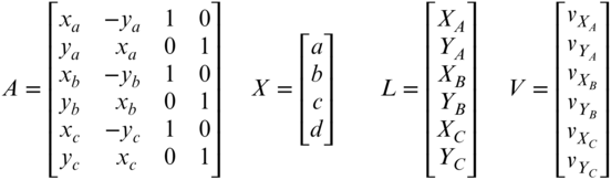
The redundant system of equations is solved using Equation (11.32). Having obtained the most probable values for the coefficients from the least squares solution, the XY coordinates for any additional points whose coordinates are known in the xy system are obtained by applying Equations (18.5) (where the residuals are now considered to be zeros).
After the adjustment, the scale factor S and rotation angle θ are computed with the following equations.

18.5 TWO-DIMENSIONAL AFFINE COORDINATE TRANSFORMATION
![]() The two-dimensional affine coordinate transformation is also known as the six-parameter transformation. It is a slight variation from the two-dimensional conformal transformation. In the affine transformation there is the additional allowance for two different scale factors; one in the x direction and the other in the y direction. This transformation is commonly used in photogrammetry for interior orientation. That is, it is used to transform photo coordinates from an arbitrary measurement photo coordinate system to the camera fiducial coordinate system, and thus account for the differential shrinkages that can occur in the x and y directions. As in the conformal transformation, the affine transformation also applies two translations of the origin, and a rotation about the origin, plus a small nonorthogonality correction between the x and y axes. This results in a total of six unknowns. The observation equations for the affine transformation are
The two-dimensional affine coordinate transformation is also known as the six-parameter transformation. It is a slight variation from the two-dimensional conformal transformation. In the affine transformation there is the additional allowance for two different scale factors; one in the x direction and the other in the y direction. This transformation is commonly used in photogrammetry for interior orientation. That is, it is used to transform photo coordinates from an arbitrary measurement photo coordinate system to the camera fiducial coordinate system, and thus account for the differential shrinkages that can occur in the x and y directions. As in the conformal transformation, the affine transformation also applies two translations of the origin, and a rotation about the origin, plus a small nonorthogonality correction between the x and y axes. This results in a total of six unknowns. The observation equations for the affine transformation are

These equations are linear and can be solved uniquely when three control points exist since each control point results in an equation set in the form of Equations (18.9). Thus, three points yield six equations involving six unknowns. If more than three control points are available, a least squares solution can be obtained. Assume, for example, that four common points (1, 2, 3, and 4) exist. Then the equation system would be

In matrix notation, Equations (18.10) are expressed as AX = L + V where

The most probable values for the unknown parameters are computed using least squares Equation (11.32). They are then used to transfer the remaining points from the xy coordinate system to the XY coordinate system. The two different rotations and scale factors can be computed from these parameters as follows:
Rotation of the measurement system, ![]()
Let t be: ![]()
Nonorthogonality of the measurement axes, α: ![]()
Scale in x, ![]()
Scale in y, ![]()
18.6 THE TWO-DIMENSIONAL PROJECTIVE COORDINATE TRANSFORMATION
![]() The two-dimensional projective coordinate transformation is also known as the eight-parameter transformation. It is appropriate to use when one two-dimensional coordinate system is projected onto another nonparallel system. This transformation is commonly used in photogrammetry and can also be used to transform NAD 27 coordinates into the NAD 83 system. In their final form, the two-dimensional projective coordinate observation equations are
The two-dimensional projective coordinate transformation is also known as the eight-parameter transformation. It is appropriate to use when one two-dimensional coordinate system is projected onto another nonparallel system. This transformation is commonly used in photogrammetry and can also be used to transform NAD 27 coordinates into the NAD 83 system. In their final form, the two-dimensional projective coordinate observation equations are

Upon inspection, it can be seen that these equations are similar to the affine transformation. In fact, if a3 and b3 are equal to zero, these equations are the affine transformation. With eight unknowns, this transformation requires a minimum of four control points. If there are more than four control points, the least squares solution may be used. Since these are nonlinear equations, they must be linearized and solved using Equation (11.37) or (11.39). The linearized form of these equations is

where

For each control point, a set of equations of the form in Equation (18.13) can be written. A redundant system of equations can be solved by least squares to yield the eight unknown parameters. With these values, the remaining points in the xy coordinate system are transformed into the XY system using Equation (18.12).
18.7 THREE-DIMENSIONAL CONFORMAL COORDINATE TRANSFORMATION
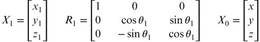
![]() The three-dimensional conformal coordinate transformation is also known as the seven-parameter similarity transformation. It transfers points from one three-dimensional coordinate system to another. It is applied in the process of reducing data from GNSS surveys and is also used extensively in photogrammetry and laser scanning. The three-dimensional conformal coordinate transformation involves seven parameters, three rotations, three translations, and one scale factor. The rotation matrix is developed from three consecutive two-dimensional rotations about the x, y, and z axes, respectively. Given in sequence, these are as follows.
The three-dimensional conformal coordinate transformation is also known as the seven-parameter similarity transformation. It transfers points from one three-dimensional coordinate system to another. It is applied in the process of reducing data from GNSS surveys and is also used extensively in photogrammetry and laser scanning. The three-dimensional conformal coordinate transformation involves seven parameters, three rotations, three translations, and one scale factor. The rotation matrix is developed from three consecutive two-dimensional rotations about the x, y, and z axes, respectively. Given in sequence, these are as follows.
In Figure 18.4, the rotation θ1 about the x axis expressed in matrix form is

FIGURE 18.4 θ1 rotation.
where
In Figure 18.5, the rotation θ2 about the y axis expressed in matrix form is

FIGURE 18.5 θ2 rotation.
where

In Figure 18.6, the rotation θ3 about the z axis expressed in matrix form is

FIGURE 18.6 θ3 rotation.
where

Substituting (a) into (b) and in turn into (c) yields
The three matrices R3, R2, and R1 in (d), when multiplied together develop a single rotation matrix R for the transformation whose individual elements are

where

Since the rotation matrix is orthogonal, it has the property that its inverse is equal to its transpose. Using this property and multiplying the terms of the matrix X by a scale factor, S, and adding translations factors Tx, Ty, and Tz to translate to a common origin yields the following mathematical model for the transformation

Equations (18.15) involve seven unknowns (S, θ1, θ2, θ3, Tx, Ty, Tz). For a unique solution, seven equations must be written. This requires a minimum of two control stations with known XY coordinates and also xy coordinates, plus three stations with known Z and z coordinates. If there is more than the minimum number of control points, a least squares solution can be used. Equations (18.15) are nonlinear in their unknowns, and thus must be linearized for a solution. The following linearized observation equations can be written for each point as

where

Note that in this adjustment, with four control points available having X, Y, and Z coordinates, 12 equations could be written, three for each point. With seven unknown parameters, this gave 12 − 7 = 5 degrees of freedom in the solution.
18.8 STATISTICALLY VALID PARAMETERS
![]() Besides the coordinate transformations described in preceding sections, it is possible to develop numerous others. For example, polynomial equations of various degrees could be used to transform data. As additional terms are added to a polynomial, the resulting equation will force better fits on any given set of data. However, caution should be exercised when doing this since the resulting transformation parameters may not be statistically significant.
Besides the coordinate transformations described in preceding sections, it is possible to develop numerous others. For example, polynomial equations of various degrees could be used to transform data. As additional terms are added to a polynomial, the resulting equation will force better fits on any given set of data. However, caution should be exercised when doing this since the resulting transformation parameters may not be statistically significant.
As an example, when using a two-dimensional conformal coordinate transformation with a data set having four control points, nonzero residuals would be expected. However, if a projective transformation were used, this data set would yield a unique solution, and thus the residuals would be zero. Is the projective a more appropriate transformation for this data set? Is this truly a better fit? Guidance in the answers to these questions can be obtained by checking the statistical validity of the derived parameters.
The adjusted parameters divided by their standard deviations represent a t statistic with ![]() degrees of freedom. If a parameter is to be judged as statistically different from zero, and thus significant, the computed t value (the test statistic) must be greater than
degrees of freedom. If a parameter is to be judged as statistically different from zero, and thus significant, the computed t value (the test statistic) must be greater than ![]() . Simply stated, the test statistic is
. Simply stated, the test statistic is
For example in the adjustment in of Example 18.2, the following computed t values are found
| Parameter | S | t value |
| a = 25.37152 | ±0.02532 | 1002.0 |
| b = 0.82220 | ±0.02256 | 36.4 |
| c = −137.183 | ±0.203 | 675.8 |
| d = −0.80994 | ±0.02335 | 34.7 |
| e = 25.40166 | ±0.02622 | 968.8 |
| f = −150.723 | ±0.216 | 697.8 |
In this problem, there were eight equations involving six unknowns and thus two degrees of freedom. From the t distribution table (Table D.3), t0.025,2 = 4.303. Because all computed t values are greater than 4.303, each parameter is significantly different from zero at a 95% level of confidence. From the adjustment results of Example 18.3, the computed t values are listed below.
| Parameters | Value | S | t value |
| a1 | 25.00274 | 0.01538 | 1626.0 |
| b1 | 0.80064 | 0.01896 | 42.3 |
| c1 | −134.715 | 0.377 | 357.3 |
| a2 | −8.00771 | 0.00954 | 839.4 |
| b2 | 24.99811 | 0.01350 | 1851.7 |
| c2 | −149.815 | 0.398 | 376.4 |
| a3 | 0.00400 | 0.00001 | 400.0 |
| b3 | 0.00200 | 0.00002 | 100.0 |
This adjustment has eight unknown parameters and 12 observations. From the t-distribution table (Table D.3), t0.025,4 = 2.776. By comparing the tabular t value against each computed value, all parameters are significantly different from zero at a 95% confidence level. This is true for a3 and b3 even though they seem relatively small at 0.004 and 0.002, respectively.
Using this statistical technique, a check can be made to determine whether the projective transformation is appropriate for a particular set of data since it will default to an affine transformation when a3 and b3 are both statistically equal to zero. Similarly if the confidence intervals for the means of a and b at a selected probability level of the two-dimensional conformal coordinate transformation contain two of the parameters from the affine transformation, then the computed values of the affine transformation are statistically the equal to those from the conformal transformation. Thus, if the interval for the population mean of a from the conformal transformation contains both a and e parameters from the affine transformation, then there is no statistical difference between these parameters. This must also be true for the population mean of b from the conformal transformation when compared to absolute values of b and d from the affine transformation. Note that a negative sign is part of the mathematical model for the conformal coordinate transformation, and thus b and d parameters are opposite in signs typically. If both of these conditions exist, then conformal transformation is the more appropriate adjustment to use for the given data since it involves fewer parameters and provides more redundant observations. One should always use the minimum number of unknown parameters to solve any problem.
A statistical test can be performed to check the parameters individually against their respective conformal-transformation parameters. This test assumes that the sample data come from populations having the same variance. Since, in this example, the same data are being used, this assumption is valid. A two-tailed test should be used. The test setup is

Test statistic:  where
where 
Rejection region: ![]() where
where ![]()
PROBLEMS
Note: For problems requiring least squares adjustment, if a computer program is not distinctly specified for use in the problem, it is expected that the least squares algorithm will be solved using the program MATRIX, which is available on the book's companion website. Partial answers to problems marked with an asterisk are given in Appendix H.
- 18.1 Points A, B, C, and D have their coordinates known in both an XY system and a xy system. Points E and F have their coordinates known only in the xy system. These coordinates are shown in the table below. Using a two-dimensional conformal coordinate transformation, determine the
- *(a) Transformation parameters and their standard deviations.
- (b) Most probable coordinates and their standard deviations for E and F in the XY coordinate system.
- *(c) Rotation angle and scale factor.
Control Points Observed Points Point X Y x y Sx Sy A −112.442 −112.113 −59.510 −147.214 0.0028 0.0024 B −112.485 112.082 −147.366 59.037 0.0029 0.0027 C 112.398 112.097 59.522 147.143 0.0027 0.0026 D 112.102 −112.436 147.206 −59.555 0.0025 0.0025 E −102.284 −46.885 0.0024 0.0025 F −43.765 103.186 0.0029 0.0025 - 18.2 Points A, B, C, and D have their coordinates known in both a (X, Y) coordinate system and an arbitrary (x, y) system. Points E, F, and G have their coordinates known only in the xy system. These coordinates are shown in the following table. Using a two-dimensional conformal coordinate transformation, determine the
- (a) transformation parameters and their standard deviations.
- (b) most probable coordinates and their standard deviations for E, F, and G in the XY coordinate system.
- (c) rotation angle and scale factor.
Control Points Observed Points Point X Y x y Sx Sy A 1766.755 1060.632 1692.046 1174.951 0.0462 0.0481 B 707.177 707.090 622.726 816.501 0.0462 0.0503 C 1060.714 1767.799 980.701 1886.112 0.0484 0.0472 D 1414.180 1414.228 1336.870 1530.531 0.0637 0.0476 E 566.519 1172.078 0.0462 0.0503 F 1423.505 1617.175 0.0462 0.0503 G 1334.658 1250.912 0.0484 0.0472 - 18.3 Repeat Problem 18.1 parts a and b using a two-dimensional affine coordinate transformation. Determine if all the parameters are statistically significant at a 5% level of significance, and use Method 1 to determine if the affine transformation is significantly different from the conformal transformation used in Problem 18.1 at a 0.05 level of significance.
- 18.4 Repeat Problem 18.3 with the data from Problem 18.2, but use Method 2 to determine if the transformations are statistically different.
- 18.5 Using a two-dimensional projective coordinate transformation and the data listed below, determine the
- *(a) transformation parameters.
- (b) most probable coordinates for 9 and 10 in the XY coordinate system.
Observed Points Control Points Point x y X Y 1 177.562 ± 0.010 −39.647 ± 0.009 −106.005 −105.902 2 138.835 ± 0.010 35.597 ± 0.010 105.995 106.154 3 −69.851 ± 0.010 −531.386 ± 0.010 −105.965 105.940 4 44.499 ± 0.013 −108.903 ± 0.010 105.696 −105.990 5 90.823 ± 0.011 −201.408 ± 0.010 −112.005 −0.026 6 97.382 ± 0.011 −29.917 ± 0.010 111.940 −0.110 7 217.344 ± 0.010 242.207 ± 0.010 0.065 112.090 8 −198.417 ± 0.010 −254.362 ± 0.009 −0.006 −111.993 9 168.454 ± 0.010 132.710 ± 0.009 10 225.533 ± 0.010 −347.645 ± 0.009 - 18.6 Do Problem 18.5 using a two-dimensional affine coordinate transformation. Determine the
- (a) transformation parameters.
- (b) most probable coordinates for 9 and 10 in the XY coordinate system.
- 18.7 Do Problem 18.5 using a two-dimensional conformal coordinate transformation. Determine the
- *(a) transformation parameters.
- (b) most probable coordinates for 9 and 10 in the XY coordinate system.
- *18.8 Determine the appropriate two-dimensional transformation for Problem 18.5 at a 0.01 level of significance.
- 18.9 Using a two-dimensional affine coordinate transformation and the following data, determine the
- (a) transformation parameters and their standard deviations.
- (b) most probable XY coordinates and their standard deviations for points 9 and 10.
Point x y X Y 1 110.299 ± 0.030 223.770 ± 0.020 −113.0003 0.0024 2 189.312 ± 0.031 318.053 ± 0.027 −105.9607 105.5976 3 284.184 ± 0.029 397.601 ± 0.027 0.0021 112.9936 4 369.095 ± 0.033 464.989 ± 0.028 105.9974 105.9964 5 301.569 ± 0.038 380.021 ± 0.031 112.8857 −0.0031 6 222.348 ± 0.039 285.493 ± 0.027 105.8891 −105.9349 7 127.803 ± 0.025 206.276 ± 0.030 −0.0015 −112.9843 8 43.234 ± 0.034 139.272 ± 0.024 −105.8870 −105.6290 9 60.902 ± 0.026 153.553 ± 0.022 10 191.255 ± 0.031 274.046 ± 0.042 - 18.10 Using a two-dimensional projective coordinate transformation, do Problem 18.9. Determine the
- (a) transformation parameters.
- (b) most probable coordinates for 9 and 10 in the XY coordinate system.
- 18.11 For the data of Problem 18.9, which two-dimensional transformation is most appropriate, and why? Use a 0.01 level of significance.
- 18.12 Determine the appropriate two-dimensional coordinate transformation for the following data at a 0.01 level of significance when transforming the XY coordinates into the EN coordinate system.
Point E (m) N (m) X (mm) Y (mm) Sx (mm) Sy (mm) 1 291,360.253 241,034.672 89.747 91.006 ±0.005 ±0.005 2 307,234.546 210,935.117 39.967 0.014 ±0.006 ±0.005 3 296,293.531 194,422.039 −20.410 0.031 ±0.006 ±0.005 4 320,061.348 206,453.166 50.161 −40.125 ±0.005 ±0.005 5 341,823.531 215,435.048 109.608 −80.316 ±0.006 ±0.005 6 259,874.536 186,836.945 −100.971 79.819 ±0.005 ±0.006 - 18.13 A survey is connected to a map projection through five stations yielding the following data.
- (a) Using Method 2, determine whether the two-dimensional transformation should be conformal or affine.
- (b) Using the appropriate transformation, determine the map projection coordinates for stations 6 and 7.
Station E (m) N (m) X (ft) Y (ft) Sx (ft) Sy (ft) 1 297,095.673 447,714.614 5,122.06 10,989.68 ±0.024 ±0.032 2 297,634.665 449,032.907 5,494.73 6,332.02 ±0.023 ±0.032 3 296,089.372 449,935.376 11,355.01 5,976.37 ±0.033 ±0.029 4 294,887.784 450,236.082 15,318.28 6,874.03 ±0.034 ±0.027 5 294,776.577 449,077.555 13,929.50 10,430.82 ±0.032 ±0.024 6 8,865.20 8,466.09 ±0.028 ±0.033 7 10,449.35 8,330.68 ±0.030 ±0.031 - 18.14 Using a level of significance of 0.01, which two-dimensional adjustment is appropriate for the following set of data?
Point X Y x y Sx Sy 1 286.94 153.23 1.484 1.530 0.044 0.046 2 299.94 162.98 10.556 5.936 0.052 0.053 3 291.48 164.11 1.641 10.558 0.052 0.041 4 296.81 166.21 6.014 10.468 0.055 0.045 5 302.18 168.41 10.591 10.386 0.051 0.043 6 299.95 162.98 10.490 5.908 0.053 0.049 7 297.66 157.53 10.390 1.555 0.053 0.051 - 18.15 Repeat Problem 18.14 with the following set of data.
Point X Y x y Sx Sy 1 215.83 62.48 88.998 92.996 ±0.008 ±0.007 2 127.71 32.27 56.011 41.997 ±0.010 ±0.009 3 9.62 97.75 −30.991 28.005 ±0.008 ±0.008 4 43.92 −69.54 53.995 −43.997 ±0.008 ±0.007 5 64.60 −187.12 112.014 −96.009 ±0.007 ±0.008 6 −21.61 239.23 −103.999 87.992 ±0.007 ±0.008 7 −168.60 −0.11 −83.004 −93.987 ±0.008 ±0.010 - 18.16 Using a weighted three-dimensional conformal coordinate transformation determine the transformation parameters and their standard deviations for the following data set.
Control Points
Point E (m) N (m) H (m) 1 205,164.469 304,594.279 704.854 2 206,136.407 304,465.336 801.905 3 203,844.790 304,119.963 734.595 4 205,375.205 303,969.042 826.081 5 206,259.276 304,204.779 765.483 Measured Points
Point e (m) n (m) h (m) Sx (m) Sy (m) Sz (m) 1 1094.961 810.073 804.720 0.030 0.031 0.033 2 508.350 1595.668 901.727 0.033 0.032 0.029 3 2356.262 197.087 834.482 0.033 0.032 0.035 4 1395.162 1397.651 925.925 0.029 0.034 0.037 5 608.992 1865.577 865.380 0.034 0.031 0.033 - 18.17 Using a weighted three-dimensional conformal coordinate transformation and the follow set of data, determine the
- (a) Transformation parameters and their standard deviations.
- (b) Compute the XYZ coordinates and their standard deviations for those points 7 and 8.
Control Stations
Station E (ft) N (ft) h (ft) 1 219,443.00 368,197.08 3,571.03 2 234,970.98 384,596.81 3 261,702.80 330,626.39 4,946.57 4 216,837.18 435,443.53 2,930.39 5 3,114.83 Measured Stations
Station e (m) n (m) H (m) Se (m) Sn (m) SH (m) 1 9,845.091 16,911.903 1,057.279 ±0.033 ±0.029 ±0.030 2 16,441.120 14,941.898 1,169.101 ±0.030 ±0.028 ±0.033 3 5,433.242 250.807 1,476.544 ±0.024 ±0.031 ±0.030 4 27,781.032 26,864.601 861.996 ±0.032 ±0.029 ±0.029 5 8,543.372 22,014.387 1,139.236 ±0.027 ±0.036 ±0.032 6 4,140.043 24,618.102 918.231 ±0.034 ±0.032 ±0.028 7 23,124.965 4,672.241 1,351.714 ±0.028 ±0.032 ±0.029 8 4,893.819 12,668.861 1,679.214 ±0.021 ±0.032 ±0.025 - 18.18 Repeat Problem 18.17 with the following data. Control Stations
Station E (m) N (m) h (m) 1 648,310.393 452,394.453 170.062 2 131.926 3 645,324.766 452,557.056 4 647,117.161 453,846.222 161.601 5 167.270 6 645,324.746 452,556.980 Measured Stations
Station x (ft) y (ft) H (ft) Sx (ft) Sy (ft) SH (ft) 1 6,019.68 5,163.17 210.33 ±0.033 ±0.024 ±0.033 2 5,901.12 11,192.94 85.11 ±0.029 ±0.037 ±0.030 3 12,591.53 12,446.33 120.16 ±0.033 ±0.031 ±0.030 4 12,184.77 5,214.17 182.42 ±0.031 ±0.026 ±0.029 5 5,901.06 11,192.99 201.02 ±0.030 ±0.034 ±0.032 6 12,591.29 12,446.47 153.12 ±0.020 ±0.030 ±0.029 7 12,184.99 5,214.33 95.35 ±0.027 ±0.027 ±0.030 8 9,728.88 7,873.23 132.99 ±0.027 ±0.030 ±0.029 Use the program ADJUST to do each problem.
- 18.19 Problem 18.4.
- 18.20 Problem 18.14.
- 18.21 Problem 18.17.
PROGRAMMING PROBLEMS
Develop a computational program that calculates the coefficient and constants matrix for each transformation.
- 18.22 A two-dimensional conformal coordinate transformation.
- 18.23 A two-dimensional affine coordinate transformation.
- 18.24 A two-dimensional projective coordinate transformation.
- 18.25 A three-dimensional conformal coordinate transformation.