
CHAPTER 12
ADJUSTMENT OF LEVEL NETS
12.1 INTRODUCTION
Differential leveling observations are used to determine differences in elevations between stations. As with all observations, these measurements are subject to random errors that can be adjusted using the method of least squares. In this chapter, the observation equation method for adjusting differential leveling observations by least squares is developed, and several examples are given to illustrate the adjustment procedures.
12.2 OBSERVATION EQUATION
![]() To apply the method of least squares in leveling adjustments, a prototype observation equation is first written for any elevation difference. Figure 12.1 illustrates the functional relationship for an observed elevation difference between two stations I and J. The equation is expressed as
To apply the method of least squares in leveling adjustments, a prototype observation equation is first written for any elevation difference. Figure 12.1 illustrates the functional relationship for an observed elevation difference between two stations I and J. The equation is expressed as
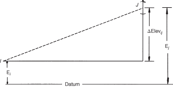
FIGURE 12.1 Differential leveling observation.
This prototype observation equation relates the unknown elevations of any two stations, I and J, with the differential leveling observation ΔElevij and its residual ![]() . This equation is fundamental in performing least squares adjustments of differential level nets.
. This equation is fundamental in performing least squares adjustments of differential level nets.
12.3 UNWEIGHTED EXAMPLE
In Figure 12.2, a leveling network and its survey data are shown. Assume that all observations are equal in weight. In this figure, arrows indicate the direction of leveling and thus, for line 1, leveling proceeds from bench mark X to A with an observed elevation difference of +5.10 ft. By substituting into prototype Equation (12.1), an observation equation is written for each observation in Figure 12.2. The resulting equations are


FIGURE 12.2 Interlocking leveling network.
Rearranging so that the known bench marks are on the right-hand side of the equations and substituting in their appropriate elevations yields

In this example, there are three unknowns, A, B, and C. In matrix form, Equations (12.2) are written as
where
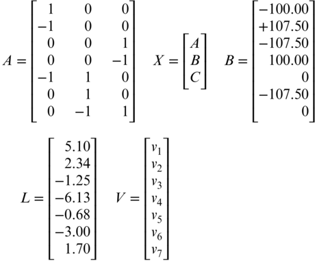
In Equation (12.4a), the B matrix is a vector of the constants (bench marks) collected from the left-side of the equation and L a collection of leveling observations. The right side of the Equation (12.3) is equal to L − B. It is a collection of the constants in the observation equations and is often referred to as the constants matrix, L. Since the bench marks can be also thought of as observations, this combination of bench marks and leveling observation is referred to as L in this book and Equation (12.4a) is simplified as
Also note in the A matrix that when an unknown does not appear in an equation, its coefficient is zero. Since this is an unweighted example, according to Equation (11.31) the normal equations are
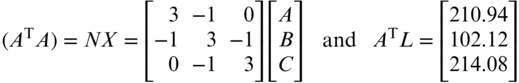
Using Equation (11.32), the solution of Equation (12.5) is
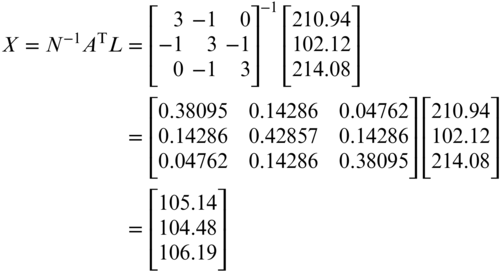
From Equation (12.6), the most probable elevations for A, B, and C are 105.14, 104.48, and 106.19, respectively. The rearranged form of Equation (12.4b) is used to compute the residuals as
From Equation (12.7), the matrix solution for V is

12.4 WEIGHTED EXAMPLE
![]() In Section 10.6, it was shown that relative weights for adjusting level lines are inversely proportional to the lengths of the lines:
In Section 10.6, it was shown that relative weights for adjusting level lines are inversely proportional to the lengths of the lines:

The application of weights to the least squares adjustment of the level circuit is illustrated by including the variable line lengths for the unweighted example of Section 12.3. These line lengths for the leveling network of Figure 12.2 and their corresponding relative weights are given in Table 12.1. For convenience, each length is divided into the constant 12, so that integer “relative weights” were obtained. (Note that this is an unnecessary step in the adjustment.) The observation equations are now formed as in Section 12.3, except that in the weighted case, each equation is multiplied by its weight.

TABLE 12.1 Weights for Example in Section 12.2
| Line | Length (mi) | Relative Weights |
| 1 | 4 | 12/4 = 3 |
| 2 | 3 | 12/3 = 4 |
| 3 | 2 | 12/2 = 6 |
| 4 | 3 | 12/3 = 4 |
| 5 | 2 | 12/2 = 6 |
| 6 | 2 | 12/2 = 6 |
| 7 | 2 | 12/2 = 6 |
After dropping the residual terms in Equation (12.9), they can be written in terms of matrices as

Applying Equation (11.34), we find the normal equations are
where

By using Equation (11.35), the solution for the X matrix is

The residual equation [Equation (12.7)] is now applied to compute the residuals as

It should be noted that these adjusted values (X matrix) and residuals (V matrix) differ slightly from those obtained in the unweighted adjustment of Section 12.3. This illustrates the effect of weights in an adjustment. Although the differences in this example are small, for precise level circuits it is both logical and wise to use a weighted adjustment since a correct stochastic model will place the errors back in the observations that most likely produced the errors.
12.5 REFERENCE STANDARD DEVIATION
Equation (10.20) expressed the standard deviation for a weighted set of observations as

However, Equation (12.13) applies to a set of multiple observations for a single quantity where each observation has a different weight. Often, observations are obtained that involve several unknown parameters that are related functionally like those in Equations (12.3) or (12.9). For these types of observations, the standard deviation in the unweighted case is

In Equation (12.14), Σv2 is expressed in matrix form as VTV, m the number of observations, and n the number of unknowns. There are r = m − n redundant measurements or degrees of freedom.
The standard deviation for the weighted case is

where ![]() in matrix form is VTWV.
in matrix form is VTWV.
Since these standard deviations relate to the overall adjustment and not a single quantity, they are referred to as reference standard deviations. Computation of the reference standard deviations for both unweighted and weighted examples is illustrated below.
12.5.1 Unweighted Example
In the example of Section 12.3, there are 7 – 3, or 4 degrees of freedom. Using the residuals given in Equation (12.7) and using Equation (12.14), the reference standard deviation in the unweighted example is
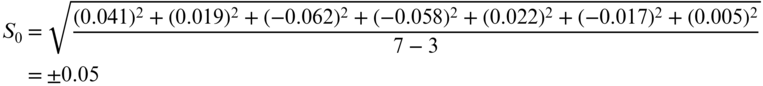
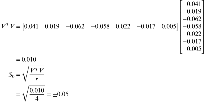
This can be computed using the matrix expression in Equation (12.14) as
12.5.2 Weighted Example
Notice that the weights are used when computing the reference standard deviation in Equation (12.15). That is, each residual is squared and multiplied by its weight, and thus the reference standard deviation computed using nonmatrix methods is

It is left as an exercise to verify this result by solving the matrix expression of Equation (12.15).
12.6 ANOTHER WEIGHTED ADJUSTMENT
12.7 SOFTWARE
The example files presented in this chapter are solved in spreadsheet format in the file Chapter 12.xls, which is available on the companion website for this book. This file demonstrates how least squares solutions can be solved in a spreadsheet. Additionally, for Example 12.1 an example of the data created in the spreadsheet is set up for copying to the MATRIX software, which is also available on the website. This file is shown in Figure 12.4. All of the examples shown in this chapter are solved in the Mathcad® file C12.xmcd, which are available on the companion website. This file demonstrates how to solve differential leveling problems using a higher-level programming language. For Example 12.1, the file shows how to read a differential leveling and create formatted results in Mathcad®.

FIGURE 12.4 MATRIX file for Example 12.1.

FIGURE 12.6 Differential leveling least squares options in ADJUST.
Furthermore, files for solving Example 12.1 in MATRIX and ADJUST are available on the companion website. The data files for both programs are simple text files with specific formats, which can be created with the editors supplied in each program. The data file for MATRIX is called Matrix file for Example 12-1.Mdat and is shown in Figure 12.4. It has the following format. The first line is a title line and can contain any description up to 80 characters in length. The second line contains the name of the first matrix, which is A in this file. This is followed by the dimensions of the matrix, then each row of the A matrix. Following the entry of the A matrix, the weight matrix W and constants matrix L are entered in a similar fashion. A space delimits each entry in the file. These entries can also be delimited by a tab or comma. The tab is a common delimiter for data copied from a spreadsheet. This feature allows for quick solution of least squares problems.
Figure 12.5 shows the format for ADJUST file used to solve Example 12.1. The format of this file is a file description line, followed by a line containing the number of control bench marks, elevation differences, and the total number of stations in the file. Following these lines are lines containing the control bench mark identifiers and elevations. All station identifiers in this file can have 10 alphanumeric characters, but may not contain a space, comma, or tab, which are reserved as delimiters between entries in the file. Following the entry of control bench marks, the observed elevation differences are listed. Each elevation difference is entered as I J ΔElev, which is the from station, to station, and observed difference in elevation. When the standard deviation, number of setups between stations, or distance between stations is known, it can be entered at the end of each observation's line for use in a weighted adjustment. Once this file is saved, the differential leveling least squares adjustment option can be run from the programs menu of ADJUST. As shown in Figure 12.6, you can select the appropriate adjustment options for the data. If distances or the number of setups is used to develop a stochastic model in a weighted adjustment, the first option in Figure 12.6 should be selected. If standard deviations or an unweighted adjustment is desired, the first option should not be selected. Many of the remaining options for this program will be discussed in later chapters. However, if the print matrices option is selected, the software will create a separate file having a mat extension, which will contain several matrices including the A and L. These matrices can be used to check those developed by the reader in the solution of a problem.
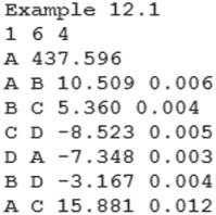
FIGURE 12.5 ADJUST file for Example 12.1.
PROBLEMS
Note: For problems requiring least squares adjustment, if a computer program is not distinctly specified for use in the problem, it is expected that the least squares algorithm will be solved using the program MATRIX, which is available on the companion website for this book. Partial answers to problems marked with an asterisk can be found in Appendix H.
- *12.1 For the leveling network in the accompanying figure calculate the most probable elevations for X and Y. Use an unweighted least squares adjustment with the observed values given in the accompanying table. Assume units of feet.
Line ΔElev (ft) 1 +3.68 2 +2.06 3 −2.02 4 −2.37 5 −0.38 
- *12.2 For Problem 12.1, compute the reference standard deviation and tabulate the adjusted observations and their residuals.
- 12.3 Repeat Problem 12.1 using ADJUST.
- 12.4 For the leveling network shown in the accompanying figure, calculate the most probable elevations for X, Y, and Z. The observed values and line lengths are given in the table. Apply appropriate weights in the computations.
Line ΔElev (ft) Length (ft) 1 +13.46 2300 2 −16.48 2300 3 −11.32 1300 4 +8.35 1300 5 +3.01 1250 6 −3.00 400 
- 12.5 For Problem 12.4, compute the reference standard deviation, and tabulate the adjusted observations and their residuals.
- 12.6 Repeat Problem 12.4 and 12.5 using the following standard deviations for the lines.
Line S (ft) 1 ±0.031 2 ±0.031 3 ±0.025 4 ±0.025 5 ±0.016 6 ±0.025 - (a) Tabulate the most probable values for the adjusted bench marks.
- (b) Tabulate the adjusted observations and their residuals.
- (c) What is the reference standard deviation for the adjustment?
- 12.7 Repeat Problem 12.6 for the following set of data.
Line ΔElev (m) S (mm) Line ΔElev (m) S (mm) 1 26.330 ±7.9 4 −22.280 ±5.6 2 −33.560 ±7.9 5 7.040 ±3.6 3 15.120 ±5.6 6 −6.970 ±5.6 - *12.8 A line of differential level is run from bench mark Oak (elevation 753.01) to station 13+00 on a proposed alignment. It continued along the alignment to 19+00. Rod readings were taken on stakes at each full station. The circuit then closed on bench mark Bridge having an elevation of 764.95 ft. The observed elevation differences, in order, are −3.03, 4.10, 4.03, 7.92, 7.99, −6.00, −6.02, and 2.98 ft. A third tie between bench mark Rock (elevation of 772.39 ft) and station 16+00 is observed as −6.34 ft. What are the
- (a) Most probable values for the adjusted elevations?
- (b) Reference standard deviation for the adjustment?
- (c) Adjusted observations and their residuals?
- 12.9 Use ADJUST to solve Problem 12.8.
- 12.10 Repeat Problem 12.8 using the differences in elevation between Oak (5034.56 ft) and Bridge (5039.88 ft) of −4.23, 2.73, −1.50, −2.50, 5.81, 1.18, 1.61, 2.16, and the elevation difference between Rock (5016.79 ft) and station 1600 is 12.25.
- 12.11 Repeat Problem 12.10 using standard deviations for each observation of ±0.015, ±0.011, ±0.011, ±0.011, ±0.011, ±0.011, ±0.011, ±0.011, and ±0.016, respectively.
- 12.12 If the elevation of A is 1302.243 m, adjust the following leveling data using the weighted least squares method.
From To ΔElev (m) S (mm) A B 20.846 ±6.0 B C 2.895 ±4.9 C D 6.888 ±4.9 D E −4.254 ±4.9 E F −4.498 ±6.0 F G −2.667 ±4.9 G A −19.194 ±4.9 A C 23.737 ±6.9 C F −1.876 ±8.4 F D 8.765 ±6.0 - (a) What are the most probable values for the elevations of the stations?
- (b) What is the reference standard deviation?
- (c) Tabulate the adjusted observations and their residuals.
- 12.13 Use ADJUST to solve Problem 12.12.
- 12.14 Repeat Problem 12.12 using the following observations and an elevation for A of 3456.98 ft.
From To ΔElev (ft) S (ft) A B −3.91 ±0.016 B C −3.73 ±0.016 C D 1.96 ±0.011 D E 0.80 ±0.011 E F 3.57 ±0.011 F G 2.72 ±0.011 G A −1.38 ±0.011 A C −7.62 ±0.016 C F 6.32 ±0.016 F D −4.37 ±0.016 - 12.15 If the elevation of Station 1 is 342.384 m, use weighted least squares to adjust the following leveling.
From To ΔElev (m) S (m) From To ΔElev (m) S (m) 1 2 −6.767 ±0.004 2 3 15.232 ±0.004 3 4 33.095 ±0.007 4 5 −11.873 ±0.004 5 6 −8.450 ±0.005 6 1 −21.230 ±0.004 1 7 6.002 ±0.004 7 3 2.446 ±0.007 2 7 12.785 ±0.006 7 6 15.222 ±0.003 6 3 −12.776 ±0.007 3 8 −9.745 ±0.007 8 5 30.956 ±0.008 6 8 −22.519 ±0.007 8 4 42.844 ±0.009 - (a) What are the most probable values for the elevations for the stations?
- (b) What is the adjustment's reference standard deviation?
- (c) Tabulate the adjusted observations and their residuals.
- 12.16 Use ADJUST to solve Problem 12.15.
- 12.17 Precise procedures were applied with a level that can be read to within ±0.4 mm/1 m and had a bubble sensitivity of ±0.3″. The line of sight was held to within ±1″ of horizontal, and the sight distances were 50 ± 3 m in length. Use these specifications and Equation (9.20) to compute standard deviations and hence weights. The elevation of A is 235.896 m. Adjust the network by weighted least squares.
From To ΔElev (m) Number of Setups From To ΔElev (m) Number of Setups A B 12.383 15 M D −38.238 42 B C −16.672 18 C M 30.338 39 C D −7.903 25 M B −13.676 23 D A 12.190 53 A M 26.058 30 - (a) What are the most probable values for the elevations of the stations?
- (b) What is the reference standard deviation for the adjustment?
- (c) Tabulate the adjusted observations and their residuals.
- 12.18 Repeat Problem 12.17 using the number of setups for weighting following procedures discussed in Section 10.6.
- 12.19 In Problem 12.17, the estimated error in reading the rod is 1.5 mm/100 m. The bubble sensitivity of the instrument is 1 mm/km and the average sight distances are 150 ft using Equation (9.21). What are the
- (a) Estimated standard errors for the observations?
- (b) Most probable values for the elevations of the stations?
- (c) Reference variance for the adjustment?
- (d) Tabulate the adjusted observations and their residuals.
- 12.20 Demonstrate that ∑v2 = VTV.
- 12.21 Demonstrate that ∑wv2 = VTWV.
PROGRAMMING PROBLEMS
- 12.22 Write a program that reads a file of differential leveling observations and writes the matrices A, W, and L in a format suitable for the MATRIX program. Using this package, solve Problem 12.14.
- 12.23 Write a computational package that reads the matrices A, W, and L, computes the least squares solution for the unknown station elevations, and writes a file of adjusted elevation differences and their residuals. Using this package, solve Problem 12.14.
- 12.24 Write a computational package that reads a file of differential leveling observations, computes the least squares solution for the adjusted station elevations, and writes a file of adjusted elevation differences and their residuals. Using this package, solve Problem 12.14.