
2 The Navigation Equations
2.1 INTRODUCTION
The navigation equations describe how the sensor outputs are processed in the on board computer in order to calculate the position, velocity, and attitude of the aircraft. The navigation equations contain instructions and data and are part of the airborne software that also includes moding, display drivers, failure detection, and an operating system, for example. The instructions and invariant data are usually stored in a read-only memory (ROM) at the time of manufacturing. Mission-dependent data (e.g., waypoints) are either loaded from a cockpit keyboard or from a cartridge, sometimes called a data-entry device, into random-access memory (RAM). Waypoints are often precomputed in a ground-based dispatch or mission-planning computer and transferred to the flight computers.
Figure 2.1 is the block diagram of an aircraft navigation system. The system utilizes three types of sensor information (as explained in Chapter 1):
- Absolute position data from radio aids, radar checkpoints, and satellites (based on range or differential range measurements).
- Dead-reckoning data, obtained from inertial, Doppler, or air-data sensors, as a means of extrapolating present position. A heading reference is required in order to resolve the measured velocities into the computational coordinates.
- Line-of-sight directions to stars, which measure a combination of position and attitude errors (as explained in Chapters 1 and 12).
The navigation computer combines the sensor information to obtain an estimate of the aircraft's position, velocity, and attitude. The best estimate of position is then combined with waypoint information to determine range and bearing to the destination. Bearing angle is displayed and sent to the autopilot as a steering command. Range to go is the basis of calculations, executed in a navigation or flight-management computer, that predict time of arrival at waypoints and that predict fuel consumption. Map displays, read from on-board compact discs (CD-ROM, Section 2.9), are driven by calculated position.

Figure 2.1 Block diagram of an aircraft navigation system.
2.2 GEOMETRY OF THE EARTH
The Newtonian gravitational attraction of the Earth is represented by a gravitational field G. Because of the rotation of the Earth, the apparent gravity field g is the vector sum of the gravitational and centrifugal fields (Figure 2.2):
where Ω is the inertial angular velocity of the Earth (15.04107 deg/hr) and R is the radius vector from the mass center of the Earth to a point where the field is to be computed. The direction of g is the “plumb bob,” or “astronomic” vertical [10].
In cooling from a molten mass, the Earth has assumed a shape whose surface is a gravity equipotential and is nearly perpendicular to g everywhere (i.e., no horizontal stresses exist at the surface). For navigational purposes, the Earth's surface can be represented by an ellipsoid of rotation around the Earth's spin axis. The size and shape of the best-fitting ellipsoid are chosen to match the sea-level equipotential surface. Mathematically, the center of the ellipsoid is at the mass center of the Earth, and the ellipsoid is chosen so as to minimize the mean-square deviation between the direction of gravity and the normal to the ellipsoid, when integrated over the entire surface. National ellipsoids have been chosen to represent the Earth in localized areas, but they are not always good worldwide approximations. The centers of these national ellipsoids are not exactly coincident and do not exactly coincide with the mass center of the Earth [9]. In 1996, the World Geodetic System (WGS-84, [20]) was the best approximation to the geoid, based on gravimetric and satellite observations. Reference [20] contains transformation equations that convert between WGS-84 and various national ellipsoids. The differences are typically hundreds of feet, though some isolated island grids are displaced as much as a mile from WGS-84. The navigator does not ask that the Earth be mapped onto the optimum ellipsoid. Any ellipsoid is satisfactory for worldwide navigation if all points on Earth are mapped onto it.
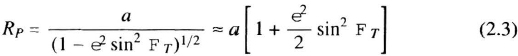
The geometry of the ellipsoid is defined by a meridian section whose semi-major axis is the equatorial radius a and whose semiminor axis is the polar radius b, as shown in Figure 2.2. The eccentricity of the elliptic section is defined as ![]() and the ellipticity, or flattening, as f = (a − b)/a.
and the ellipticity, or flattening, as f = (a − b)/a.
The radius vector R makes an angle FC with the equatorial plane, where FC is the geocentric latitude; R and FC are not directly measurable, but they are sometimes used in mechanizing dead-reckoning equations.
The geodetic latitude FT of a point is the angle between the normal to the reference ellipsoid and the equatorial plane. Geodetic latitude is our usual understanding of map latitude. The term “geographic latitude” is sometimes used synonymously with “geodetic” but should refer to geodetic latitude on a worldwide ellipsoid.
The radii of curvature of the ellipsoid are of fundamental importance to dead-reckoning navigation. The meridian radius of curvature, RM, is the radius of the best-fitting circle to a meridian section of the ellipsoid:

Figure 2.2 Meridian section of the Earth, showing the reference ellipsoid and gravity field.

The prime radius of curvature, RP, is the radius of the best-fitting circle to a vertical east–west section of the ellipsoid:
The Gaussian radius of curvature is the radius of the best-fitting sphere to the ellipsoid at any point:

The radii of curvature are important, because they relate the horizontal components of velocity to angular coordinates, such as latitude and longitude; for example,
where h is the aircraft's altitude above the reference ellipsoid, measured along the normal to the ellipsoid (nearly along the direction of gravity), and l is its longitude, measured positively east.
For numerical work a = 6378.137 km = 3443.918 nmi, f = 1/298.2572, and e2 = f(2 − f) [18]. (One nautical mile = 1852 meters exactly, or 6076.11549 ft.) The angle between the gravity vector and the normal to the ellipsoid, the deflection of the vertical, is commonly less than 10 seconds of arc and is rarely greater than 30 seconds of arc [18]. The magnitude of gravity at sea level is
within 0.02 cm/sec2. It decreases 10−6g for each 10-ft increase in altitude above sea level [16].
2.3 COORDINATE FRAMES
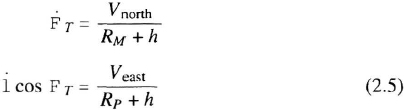
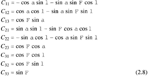
The position, velocity, and attitude of the aircraft must be expressed in a coordinate frame. Paragraph 1 below describes the rectangular Earth-centered, Earth-fixed (ECEF) coordinate frame, yi. Paragraph 2 describes the Earth-centered inertial (ECI) coordinate frame, xi, which simplifies the computations for inertial and stellar sensors. Other Earth-referenced orthogonal coordinates, called zi, can simplify navigation computations for some navaids and displays. Paragraphs 3–5 describe coordinates commonly used in inertial navigation systems. Paragraph 6 describes coordinates used in land navigators or in military aircraft that support ground troops. Paragraphs 7–9 describe coordinates that were important before powerful airborne digital computers existed.
- Earth-centered, Earth-fixed (ECEF). The basic coordinate frame for navigation near the Earth is ECEF, shown in Figure 2.3 as the yi rectangular coordinates whose origin is at the mass center of the Earth, whose y3-axis lies along the Earth's spin axis, whose y1 axis lies in the Greenwich meridian, and which rotates with the Earth [10]. Satellite-based radio-navigation systems often use these ECEF coordinates to calculate satellite and aircraft positions.
- Earth-centered inertial (ECI). ECI coordinates, xi, can have their origin at the mass-center of any freely falling body (e.g., the Earth) and are nonrotating relative to the fixed stars. For centuries, astronomers have observed the small relative motions of stars (“proper motion”) and have defined an “average” ECI reference frame [11]. To an accuracy of 10−5deg/hr, an ECI frame can be chosen with its x3-axis along the mean polar axis of the Earth and with its x1- and x2-axes pointing to convenient stars (as explained in Chapter 12). ECI coordinates have three navigational functions. First, Newton's laws are valid in any ECI coordinate frame. Second, the angular coordinates of stars are conventionally tabulated in ECI. Third, they are used in mechanizing inertial navigators, Section 7.5.1.
Figure 2.3 Navigation coordinate frames.
- Geodetic spherical coordinates. These are the spherical coordinates of the normal to the reference ellipsoid (Figure 2.2). The symbol z1 represents longitude l; z2 is geodetic latitude FT, and Z3 is altitude h above the reference ellipsoid. Geodetic coordinates are used on maps and in the mechanization of dead-reckoning and radio-navigation systems. Transformations from ECEF to geodetic spherical coordinates are given in [9] and [23].
- Geodetic wander azimuth. These coordinates are locally level to the reference ellipsoid,
 is vertically up and
  points at an angle, a, west of true north (Figure 2.3). The wander-azimuth unit vectors, z1 and z2, are in the level plane but do not point east and north. Wander azimuth is the most commonly used coordinate frame for worldwide inertial navigation and is discussed below and in Section 7.5.1.
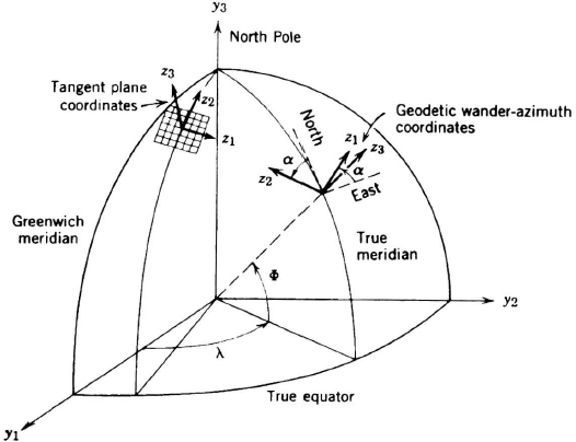
 - Direction cosines. The orientation of any z-coordinate frame (e.g., navigation coordinates or body axes) can be described by its direction cosines relative to ECEF y-axes. Any vector V can be resolved into either the y-or z-coordinate frame. The y and z components of V are related by the equation
where
The navigation computer calculates in terms of the Cij, which are usable everywhere on Earth. The familiar geographic coordinates can be found from the relations
sin F = C33,
or
wherever they converge. In polar regions, where a and l are not meaningful, the navigation system operates correctly on the basis of the Cij. Section 7.5.1 describes an inertial mechanization in direction cosines. If the z-coordinate frame has a north-pointing axis, a = 0.
- Map-grid coordinates. The navigation computer can calculate position in map-grid coordinates such as Lambert conformal or transverse Mercator xy-coordinates [13]. Grid coordinates are used in local areas (e.g., on military battlefields or in cities) but are not convenient for long-range navigation. A particular grid, Universal Transverse Mercator (UTM), is widely used by army vehicles of the western nations. The U.S. Military Grid Reference System (MGRS) consists of UTM charts worldwide except, in polar regions, polar stereographic charts [13]. The latter are projected onto a plane tangent to the Earth at the pole, from a point at the opposite pole.
- Geocentric spherical coordinates. These are the spherical coordinates of the radius vector R (Figure 2.2). The symbol z1 represents longitude l; z2 is geocentric latitude FC, and z3 is the radius. Geocentric coordinates are sometimes mechanized in short-range dead-reckoning systems using a spherical-Earth approximation. Initialization requires knowledge of the direction toward the mass center of the Earth, a direction that is not directly observable.
- Transverse-pole spherical coordinates. These coordinates are analogous to geocentric spherical coordinates except that their poles are deliberately placed on the Earth's equator. The symbol z1 represents the transverse longitude; z2, the transverse latitude; and z3, the radius. They permit non-singular operation near the north or south poles, by placing the transverse pole on the true equator. Transverse-polar coordinates involve only three zi variables instead of nine direction cosines. However, they cannot be used for precise navigation, since the transverse equator is elliptical, complicating the precise definition of transverse latitude and longitude. They are similar to but not identical to the stereographic coordinates often used in polar regions. Transverse-pole coordinates were used in inertial and Doppler navigation systems from 1955 to 1970 when primitive airborne computers required simplified computations.
- Tangent plane coordinates. These coordinates are always parallel to the locally level axes at some destination point (Figure 2.3). They are locally level only at that point and are useful for flight operations within a few hundred miles of a single destination. Here z3 lies normal to the tangent plane, and z2 lies parallel to the meridian through the origin. Section 7.5.1 describes the mechanization of an inertial navigator in tangent-plane coordinates.

2.4 DEAD-RECKONING COMPUTATIONS
Dead reckoning (often called DR) is the technique of calculating position from measurements of velocity. It is the means of navigation in the absence of position fixes and consists in calculating the position (the zi-coordinates) of a vehicle by extrapolating (integrating) estimated or measured ground speed. Prior to GPS, dead-reckoning computations were the heart of every automatic navigator. They gave continuous navigation information between discrete fixes. In its simplest form, neglecting wind, dead reckoning can calculate the position of a vehicle on the surface of a flat Earth from measurements of ground speed Vg and true heading wT:

where x − x0 and y − y0 are the east and north distances traveled during the measurement interval, respectively. Notice that a simple integration of unresolved ground speed would give curvilinear distance traveled but would be of little use for determining position.
Aircraft heading (best-available true heading) is measured using the quantities defined in Figure 2.4. With a magnetic compass, for example, the best available true heading is the algebraic sum of magnetic heading and east variation. With a gimballed inertial system, the best available true heading is platform heading (relative to the zi computational coordinates) plus the wander angle a (Section 7.5.2). When navigating manually in polar regions, dead-reckoned velocity is resolved through best available grid heading.
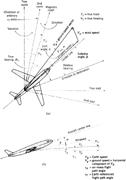
Figure 2.4 Geometry of dead reckoning.
In the presence of a crosswind the ground-speed vector does not lie along the aircraft's center line but makes an angle δ with it (Figure 2.4). The true-track angle TT, the angle from true north to the ground-speed vector, is preferred for dead-reckoning calculations when it is available. The drift angle δ can be measured with a Doppler radar or a drift sight (a downward-pointing telescope whose reticle can be rotated by the navigator to align with the moving ground).
In a moving air mass
where θ is the pitch angle, VTAS is the true airspeed and β is the sideslip angle. On a flat Earth, the north and east (or grid north and grid east) distances traveled are found by integrating the two components of velocity with respect to time. On a curved Earth, the position coordinates are not linear distances but angular coordinates. Equations 2.5 show a method for transforming linear velocities to angular coordinates. The accuracy of airspeed data is limited by errors in predicted windspeed and by errors in measuring airspeed and drift angle.
The dead-reckoning computer can process Doppler velocity. If the Doppler radar measures ground speed Vg and drift angle δ,

Equivalently, the Doppler radar can measure the components of groundspeed in body axes: ![]() along-axis and
along-axis and ![]() cross-axis (using the same symbols as in Chapter 10), both of which can be resolved through the three attitude angles, ψT, pitch and roll. Antenna misalignment relative to the heading sensor can be calibrated from a series of fixes, either in closed form or with a Kalman filter (Chapter 3).
cross-axis (using the same symbols as in Chapter 10), both of which can be resolved through the three attitude angles, ψT, pitch and roll. Antenna misalignment relative to the heading sensor can be calibrated from a series of fixes, either in closed form or with a Kalman filter (Chapter 3).
Equations 2.5 relate velocity to λ and ΨT on an ellipsoidal Earth. Similar relations can be derived for the other coordinate frames discussed in Section 2.3. The velocity with respect to Earth dR/dt|y can be expressed in zi components as follows:
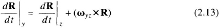
For example, in a spherical coordinate frame whose z3-axis lies along the position vector R:

where the first term is the rate of change of radius, along the radius vector, and ωyz is the angular velocity of the zi-coordinate frame relative to yi; ![]() is the unit vector in the direction of R. In direction-cosine mechanizations, the
is the unit vector in the direction of R. In direction-cosine mechanizations, the ![]() are related to the Cij by Equation 7.40, where ωi − Ωi of that equation is identical to ωyz of this one.
are related to the Cij by Equation 7.40, where ωi − Ωi of that equation is identical to ωyz of this one.
2.5 POSITIONING
2.5.1 Radio Fixes
There are five basic airborne radio measurements:
- Bearing. The angle of arrival, relative to the airframe, of a radio signal from an external transmitter. Bearing is measured by the difference in phase or time of arrival at multiple antennas on the airframe. At each bearing, the distortion caused by the airframe may be calibrated as a function of frequency. If necessary, calibration could also include roll and pitch.
- Phase. The airborne receiver measures the phase difference between continuous-wave signals emitted by two stations using a single airborne antenna. This is the method of operation of VOR azimuth and hyperbolic Omega (Chapter 4).
- Time difference. The airborne receiver measures the difference in time of arrival between pulses sent from two stations. A 10−4 clock (one part in 104) is adequate to measure the short time interval if both pulses are sent simultaneously. Because Loran pulses can be transmitted 0.1 sec apart, a clock error less than 10−6 is needed to measure the time difference. In time-differencing and phase-measuring systems (hyperbolic Loran), at least two pairs of stations are required to obtain a fix.
- Two-way range. The airborne receiver measures the time delay between the transmission of a pulse and its return from an external transponder at a known location. Round-trip propagation times are typically less than a millisecond, during which the clock must be stable. A 1% range error requires a clock-stability of 0.3% (3 × 10⁻³), which is two microseconds at 100-km range. The calculation of range requires knowledge of the propagation speed and transponder delay. DME is a two-way ranging system (Section 4.4.6).
- One-way range. The airborne receiver measures the time of arrival with respect to its own clock. If the airborne clock were synchronized with the transmitter's clock upon departure from the airfield and ran freely thereafter, a 1% range error at a distance of 100 km from a fixed station would require a clock error of one microsecond, which is 5 × 10⁻¹¹ of a five-hour mission. When 25,000-km distances to GPS satellites are to be measured with a one-meter error, a short-term clock stability of one part in 3 × 10⁸ would be needed to measure range and 10−4 seconds absolute time error would be needed to calculate the satellite's position (GPS satellites are moving at 3000 ft/sec relative to Earth). Together these would require an error of one part in 1012 for a clock synchronized with the transmitters at the start of a ten-hour mission and allowed to run freely thereafter. Only an atomic clock had this accuracy in 1996. Therefore practical one-way ranging systems use a technique called pseudoranging. The transmitters contain atomic clocks with long-term stabilities of about 10−13, while the airborne receiver's clocks have accuracies and stabilities of 10−6 to 10−9. The airborne computer solves for the aircraft's clock offset (and sometimes, drift rate) by making redundant range measurements. For example, measuring four pseudoranges obtains three-dimensional position and clock offset to a few nanoseconds using Equations 2.17 and 2.18. Pseudoranging is used in GPS and GLONASS (Chapter 5) and in one-way ranging (direct ranging) of Loran and Omega (Chapter 4).
2.5.2 Line-of-Sight Distance Measurement
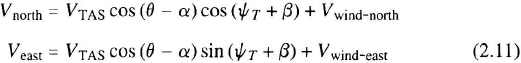
Figure 2.5 shows an aircraft near the surface of the Earth at R0 and a radio station that may be near the surface or in space, at Rsi. The slant range, |Rsi − R0|, from the aircraft to the station could be measured by one-way or two-way ranging. If ![]() is the unit local vertical vector at the aircraft, the elevation angle of the line of sight to the radio station is
is the unit local vertical vector at the aircraft, the elevation angle of the line of sight to the radio station is
Figure 2.5 Light-of-sight distance.
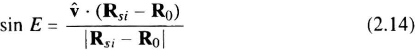
If ![]() is the unit north-pointing horizontal vector at the aircraft, the azimuth angle of the line of sight is
is the unit north-pointing horizontal vector at the aircraft, the azimuth angle of the line of sight is
These vector equations can be resolved into any coordinate frame. For example, in ECEF,

In one-way ranging systems, where the clock offset and range are to be calculated, the measured pseudorange vector from the ith station, Rim, is R0 − Rsi, corrected for the unknown offset of the airborne clock and for propagation delays in the atmosphere, expressed in distance units. The magnitude of the pseudorange in any coordinate frame (e.g., ECEF) is


The stations may be moving (e.g., satellites) or stationary (e.g., GPS pseudolites). Four pseudorange measurements are needed to solve for the four unknowns in Equations 2.17: aircraft position and clock offset. When more than four measurements are made, the equations are overdetermined so that a solution requires a model of the ranging errors, for example, using a Kalman filter (Chapter 3). The airborne computer usually solves for its position by assuming a position and clock offset, calculating the pseudoranges to four stations from Equation 2.17, comparing to the measured pseudoranges (with respect to its own clock), and iterating until the calculated and measured pseudoranges are close enough. The next iteration is chosen as follows: In the kth iteration, the assumed position is xk yk zk whose range to the ith station differs from the measured range Rim by ΔXk = Rim(k) − Rsi. The components of ΔXk in the navigation coordinates are ΔXk, ΔYk, and ΔZk. The sensitivity of Rim to position is
where ∂Rim/∂Xj are the direction cosines between the line of sight to the ith station and the jth coordinate axis and Δtk is the error in estimating clock offset. If the assumed position and clock offset were correct, ΔXk, ΔYk, ΔZk, and Δtk would be zero and ΔRik would also be zero. But if the assumed position were misestimated by ΔXk, the error along the line of sight would be the dot product of the unit vector along the line of sight with ΔXk. Thus after computing Rimk from Equation 2.17, the next iteration is Rim(k + 1) = Rim(k) + ΔXk. Iterations cease when the difference between the calculated and measured pseudorange is within the desired accuracy. A recursive filter allows a new calculation of position and clock offset after each measurement (Chapters 3 and 5). In Equation 2.17, Earth-based line-of-sight navaids use an average index of refraction η (Chapter 4), whereas satellite-based navaids, whose signals propagate mostly in vacuum, assume that η = 1 and correct for the atmosphere with a model resident in the receiver's software (Section 5.4).
2.5.3 Ground-Wave One-Way Ranging
Loran and Omega waves propagate along the curved surface of the Earth (as explained in Chapter 4). With either sensor, an aircraft can measure the time of arrival of the navigation signal from two or more stations and compute its own position as follows:
- Assume an aircraft position.
- Calculate the exact distance and azimuth to each radio transmitter using ellipsoidal Earth equations [18].
- Calculate the predicted propagation time and time of arrival allowing for the conductivity of the intervening Earth's surface and the presence or absence of the dark/light terminator between the aircraft and the station (as described in Chapter 4).
- Measure the time of arrival using the aircraft's own clock, which is usually not synchronized to the transmitter's clock.
- Calculate the difference between the measured and predicted times of arrival to each station.
- The probable position is the assumed position, offset by the vector sum of the time differences, each in the direction of its station, converted to distance.
- Assume a new aircraft position and iterate until the residual is within the allowed error.
Three or more stations are needed if the aircraft's clock is not synchronized to the Loran or Omega transmitters. If a receiver incorporated a sufficiently stable clock, only two stations would be needed for a direct-ranging fix. Two-station fixes with a synchronized clock or three-station fixes with an asynchronous clock result in two position solutions, at the intersections of two circular, each having a vortex at a transmitter. The correct position can be found by receiving an additional station or from a priori knowledge.
2.5.4 Ground-Wave Time-Differencing
An aircraft can measure the difference in time of arrival of Loran or Omega signals from two or more stations (Chapter 4). To measure the time-difference within 0.1% requires a 0.03% accuracy clock, which is less expensive than the 10−11 clock required for uncorrected one-way ranging or the 10−6 to 10−9 clock required for pseudoranging (Section 2.5.1). As in one-way ranging, the iterative procedure is based on the precise calculation of propagation time from the aircraft to each station on an ellipsoidal Earth:
- Assume an aircraft position.
- Calculate the exact range and azimuth from the assumed position to each observed radio station using ellipsoidal Earth equations [18].
- Calculate the predicted propagation time allowing for the conductivity of the intervening Earth's surface and the presence of the sunlight terminator between the aircraft and the station.
- Subtract the times to two stations to calculate the predicted difference in propagation time.
- Measure the difference in time of arrival of the signals from the two stations.
- Subtract the measured and predicted time differences to the two stations.
- Calculate the time-difference gradients from which is calculated the most probable position of the aircraft after the measurements (see Section 2.5.2 of the First Edition of this book and Chapter 4 of this book).
- Iterate until the residual is smaller than the allowed error.
2.6 TERRAIN-MATCHING NAVIGATION
These navigation systems obtain occasional updates when the aircraft overflies a patch of a few square miles, chosen for its unique profile [5]. A digital map of altitude above sea level, hs, is stored for several parallel tracks; see Figure 2.6. For example, if 0.1-nmi accuracy is desired, hs(t) must be stored in 200-ft squares sampled every 0.2 sec at 600 knots.
The aircraft measures the height of the terrain above sea level as the difference between barometric altitude (Chapter 8) and radar altitude (Chapter 10); see Figure 2.7. Each pair of height measurements and the dead-reckoning position are recorded and time-tagged.
After passing over the patch, the aircraft uses its measured velocity to calculate the profile as a function of distance along track, hm(x), and calculates the cross-correlation function between the measured and stored profiles:

Figure 2.6 Parallel tracks through terrain patch.
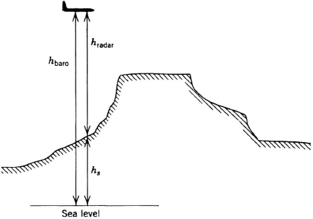
Figure 2.7 Measurement of terrain altitude.

where the map patch has a length A. The integration is long enough (n > 1) to ensure that the patch is sampled, even with the expected along-track error. The computer selects the track whose cross-correlation is largest as the most probable track. The computer selects the x-shift of maximum correlation T as the along-track correction to the dead-reckoned position. Heading drift is usually so small that correlations are not required in azimuth. The algorithm accommodates offsets in barometric altitude caused by an unknown sea-level setting. The width of the patch depends on the growth rate of azimuth errors in the dead-reckoning system. Simpler algorithms have been used (“mean absolute differences”) and more complex Kalman filters have been used [5].
Terrain correlators are built under the names TERCOM, SITAN, and TERPROM. They are usually used on unmanned aircraft (cruise missiles) and can achieve errors less than 100 ft [1, 8]. The feasibility of this navigation aid depends on the existence of unique terrain patches along the flight path and on the availability of digital maps of terrain heights above sea level. The U.S. Defense Mapping Agency produces TERCOM maps for landfalls and mid-course updates in three-arcsec grids.
2.7 COURSE COMPUTATION
2.7.1 Range and Bearing Calculation
The purpose of the course computation is to calculate range and bearing from an aircraft to one or more desired waypoints, targets, airports, checkpoints, or radio beacons. The computation begins with the best-estimate of the present position of the aircraft and ends by delivering computed range and bearing to other vehicle subsystems (Figure 2.1). Waypoints may be loaded before departure or inserted en route. The navigation computer, mission computer, or flight-management computer performs the steering calculations.
Range and bearing to a destination can be calculated by using either the spherical or the plane triangle of Figure 2.8. If flat-Earth approximations are satisfactory, the xy coordinates of the aircraft are computed using the dead-reckoning Equation 2.10; xt and yt of the targets are loaded from a cassette or from a keyboard. Then, range D and bearing BT to the target, measured from true north, are

The crew will want a display of relative bearing (BR = BT − ψT) or relative track (TR = BT − TT). BT is the true bearing of the target. Relative bearing BR is the horizontal angle from the longitudinal axis of the aircraft to the target, and relative track TR is the horizontal angle from the ground track of the aircraft to the target (Figure 2.4).
If Δλ and ΔΦ are less than ![]() radian, the plane triangle solution exceeds the spherical triangle solution by a range ΔD:
radian, the plane triangle solution exceeds the spherical triangle solution by a range ΔD:
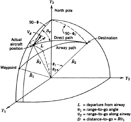
Figure 2.8 Course-line calculations.
This error is 36 nmi at a range of D = 1000 nmi, an azimuth BT = 45 deg and a latitude of Φ = 45 deg. If this is not sufficiently accurate, a spherical-triangle solution may be used:
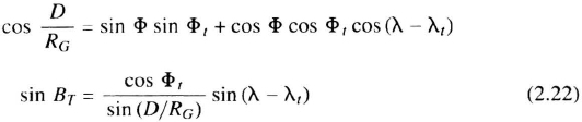
RG is the Gaussian radius of curvature, Equation 2.4. At long range, where the absolute and percent errors are largest, they are usually least significant. Within 100 nmi of the aircraft, the Earth can be assumed flat within an error of 0.3 nmi.
Steering and range-bearing computations can be performed directly from the zi navigation coordinates or from the direction cosines Cij to prevent singularities near the north and south poles.
Knowing the measured or computed ground speed, an aircraft can be steered in such a manner that the ground speed vector—not the longitudinal axis of the aircraft—tracks toward the desired waypoint (relative track is the steering command that is nulled). The difference between heading toward the target and tracking toward the target is significant only for helicopters; the vehicle eventually arrives there in either case, by slightly different paths.
Two general kinds of steering to a destination are commonly used: (1) steering directly from the present position to the destination and (2) steering along a preplanned airway or route. The former results in area navigation (Section 2.7.4) using the shortest (though not necessarily the fastest) route to the destination, whereas the latter is representative of flying along assigned airways (Chapter 14). Either steering method may be solved by the plane-triangle or spherical-triangle calculation.
The rhumb line is used by ships and simple aircraft. It is defined by flying at a constant true heading to the local meridians. The resulting flight path is a straight line on a Mercator chart. Aircraft sometimes divide a complex route into rhumb-line segments so that each segment can be flown at constant heading.
More often, the continually changing heading toward the next waypoint is recomputed and fed to the autopilot. Since the great circle maps into a near-straight line on a Lambert conformal chart, the crew can monitor the flight path by manual plotting, if desired. In the twenty-first century, electronic map displays will show the moving aircraft on charts.
2.7.2 Direct Steering
The steering computer calculates the ground speed V1 along the direction to the destination and V2 normal to the line of sight to the destination. The commanded bank angle is made proportional to V2 in order that the aircraft's heading rate ![]() be driven to zero when flying along the desired great circle. If Va is airspeed,
be driven to zero when flying along the desired great circle. If Va is airspeed, ![]() tan ϕ and the commanded bank angle is
tan ϕ and the commanded bank angle is
K2 provides some anticipation when approaching the correct direction of flight. The commanded bank angle ϕc is limited to a maximum value (e.g., 15 deg) in order to avoid violent maneuvers when the aircraft's flight direction is greatly in error.
Near the destination, the computation of lateral speed, V2, becomes singular, and the steering signal would fluctuate erratically. To prevent this, the track angle or heading is frozen and held until the destination (computed from range-to-go and ground speed) is passed. The range at which the steering must be frozen is determined by simulation. This navigation method is sometimes called proportional navigation, a term derived from missile-steering techniques in which the heading rate of the vehicle is made proportional to the line-of-sight rate to the target.
The normal to the great-circle plane connecting present position R3 to the destination R2 is defined by the unit vector ![]() :
:
(Figure 2.8). The lateral speed V2 is the magnitude of the dot product of the aircraft's velocity with this unit vector. The range to go from R3 to R2 is given by Equation (2.20) or (2.22). Time to go is calculated from the proposed velocity schedule.
The fastest route is neither the great circle nor the airway because of winds, especially because of the stratospheric jet stream whose speed often exceeds 100 knots. Thus where high-altitude aircraft are not confined to airways, they follow preplanned “pressure-pattern” routes that take advantage of cyclonic tail winds.
2.7.3 Airway Steering
The steering algorithm calculates a great circle from the takeoff point (or from a waypoint) to the destination (or to another waypoint). The aircraft is steered along this great circle by calculating the lateral deviation L (Figure 2.8) from the desired great circle and commanding a bank angle:
The integral-of-displacement term is added to give zero steady-state displacement from the airway in the presence of a constant wind and is also used in automatic landing systems (Chapter 13) in order to couple the autopilot to the localizer beam of the instrument-landing system. The bank angle is limited, to prevent excessive control commands when the aircraft is far off course. Near the destination, the track, or heading, is frozen to prevent erratic steering.
As the aircraft passes each waypoint, a new waypoint is fetched, thus selecting a new desired track. The aircraft can then fly along a series of airways connecting checkpoints or navigation stations.
The great-circle airway is defined by the waypoint vectors R1 and R2. The angle to go to waypoint 2 is:

Range and time to go are calculated as in Section 2.7.2. The lateral-deviation angle L/D is:

These computations can be performed directly in terms of the navigation coordinates zi.
2.7.4 Area Navigation
Between 1950 and approximately 1980, aircraft in developed countries flew on airways, guided by VOR bearing signals (Chapter 4). Position along the airway could be determined at discrete intersections (Δ in Figure 2.9) using cross-bearings to another VOR. In the 1970s DME, colocated with the VOR, allowed aircraft to determine their position along the airways continuously. Thereafter, regulating authorities allowed them to fly anywhere with proper clearances, a technique called RNAV (random navigation) or area navigation. RNAV uses combinations of VORs and DMEs to create artificial airways either by connecting waypoints defined by latitude/longitude or by triangulation or trilateration to VORTAC stations (as shown by the dotted lines to A1 in Figure 2.9). The on-board flight-management or navigation computer calculates the lateral displacement L from the artificial airway and the distance D to the next waypoint A1 along the airway [24b,c], [25].
In Figure 2.9, ρ1 and ρ3 are the measured distances to the DME stations at V1 and V3. The position P1 is found from the triangle P1V1V3. The aircraft's position must be known well enough to exclude the false solution at P2. An artificial airway is defined by the points A1 and A2. D and L are usually found iteratively:

Figure 2.9 Plan view of area-navigation fix.
- Assume P1 based on prior navigation information.
- Calculate the ranges ρ1 and ρ3 to the DMEs at V1 and V3 using the range equations of Section 2.5.2. A range-bearing solution relative to a single VOR station calculates the aircraft's position, but not as accurately as a range-range solution to two stations.
- Correct the measured ranges for the altitudes of the aircraft and DME station.
- Subtract the measured and calculated ranges

- The next estimate of ρ1 is along the vector Δρk in Figure 2.9, whose components along ρ1 and ρ3 are Δρ1 and Δρ3.
- Repeat step 2 and iterate until Δρi are acceptably small.
After determining the aircraft's position P1, the distance-to-go and lateral displacement are calculated as in Section 2.7. L is sent to the autopilot, as explained in Section 2.7.3, and D is used to calculate time-to-go.
In the 1990s, civil aircraft were being allowed the freedom to leave RNAV airways (Section 1.5.3) using GPS, inertial, Omega, and Loran navigation, none of which constrain aircraft to airways.
2.8 NAVIGATION ERRORS
2.8.1 Test Data
Navigation errors establish the width of commercial airways, the spacing of runways, and the risk of collision. Navigation errors determine the accuracy of delivering weapons and pointing sensors.
All navigation systems show a statistical dispersion in their indication of position and velocity. Test data can be taken on the navigation system as a whole and on its constituent sensors. Tests are conducted quiescently in a laboratory, in an artificial environment (e.g., rate table or thermal chamber), or in flight. As accuracies improve, the statistical dispersions, once considered mere noise, become important enough to predict (as discussed in Chapter 3).
The departure of a commercial aircraft from its desired flight path is sometimes divided into:
- Navigation sensor errors
- Computer errors
- Data entry errors
- Display error if the aircraft is flown by a pilot
- Flight technical error, which is the departure of the pilot-flown or autopilot-flown aircraft from the computed path
Deterministic errors are added algebraically and statistical errors are root sum squared. The total is sometimes called total system error.
The two- or three-dimensional vector position error r can be defined as indicated minus actual position. A series of measurements taken on one navigation system or on any sample of navigation systems will yield a series of position measurements that are all different but that cluster around the actual position. If the properties of the navigation systems do not change appreciably with age, if the factory is neither improving nor degrading its quality control, and if all systems are used under the same conditions, then the statistics of the series of measurements taken on any one system are the same as those taken for a sample (“ensemble”) of systems. Mathematically it is said that the statistics are ergodic and stationary.
If the position errors are plotted in two dimensions, as shown in Figure 2.10, it will generally be found that the average position error r = ΣΔri/N) is not zero (Δri are the individual position errors; N is the total number of measurements). Two measures of performance are the mean error and the circular error probability (CEP) (also known as the circular probable error, CPE). The CEP is usually considered to be the radius of a circle, centered at the actual position (but more properly centered at the mean position of a group of measurements) that encloses 50% of the measurements. The mean error and the CEP may be suitable as crude acceptance tests or specifications, but they yield little engineering information.

Figure 2.10 Two-dimensional navigation errors. In principal axes, the x and y statistics are independent.
More rigorously, the horizontal position error should be considered as a bivariate (two-dimensional) distribution. The mean error r and the directions of the principal axes x and y, for which errors in x and y are uncorrected, must be found. To find the principal axes, a convenient orthogonal coordinate system (x′, y′) is established with its origin at r. Then the standard deviation (or rms) σ in each axis and the correlation coefficient ρ between axes are calculated:

From these quantities are determined a new set of coordinates, xy, which are rotated θ from x′y′:

The origin of the new xy-coordinates coincides with the origin of x′y′. The components of the position errors along x and y are uncorrected and can be considered separately. In inertial systems, the principal axes are usually the instrument axes. In Doppler systems, the principal axes are along the velocity vector and normal to it or along the aircraft axis and normal to it if the antenna is body-fixed (as was usually the case in 1996). In Loran systems, the principal axes are found by diagonalizing the covariance matrix. The rms errors in the new coordinates can be calculated anew or can be found from the errors in x′y′ from [7, p. 598].
The one-dimensional statistics along either of the principal axes will now be discussed. First, the mean and standard deviation are found in each independent axis. The errors along each axis are plotted separately as cumulative distribution curves, which show the fraction of errors less than x versus x. This curve allows all properties of the statistics to be determined. In many systems, experimental cumulative distributions will fit a Gaussian curve.
If the one-dimensional errors are indeed Gaussian, their statistics have the following properties:
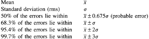
From these properties of the Gaussian distribution, it is easy to tell whether an experimentally determined cumulative distribution curve is approximately Gaussian. Reference [7] shows statistical tests for “normality” of experimental data.
Returning to the two-dimensional case, the probability that a navigation error falls within a rectangle 2m by 2n, centered at the mean and aligned with the principal axes (x and y uncorrected), is found by multiplying the tabulated error functions for m/σx and n/σy computed independently. Tables for the probability integral ([14], p. 116) can be used instead for ![]() and
and ![]() . For example, if σx = 0.4 nmi and σy = 1.0 nmi, the probability of falling inside a rectangle 1.2 nmi (in x) by 2.4 nmi (in y) is the product of the probability integrals for
. For example, if σx = 0.4 nmi and σy = 1.0 nmi, the probability of falling inside a rectangle 1.2 nmi (in x) by 2.4 nmi (in y) is the product of the probability integrals for ![]() and
and ![]() , which is 0.866 × 0.770 = 66%. Thus, the 1.2 by 2.4 nmi rectangle encloses 66% of the navigation errors.
, which is 0.866 × 0.770 = 66%. Thus, the 1.2 by 2.4 nmi rectangle encloses 66% of the navigation errors.
Navigation systems, civil and military, are often specified by the fraction of navigation errors that fall within a circle of radius ![]() , centered on the mean. Figure 2.11 shows this probability if σx and σy are Gaussian distributed and uncorrected. For example, if σx = 0.4 nmi and σy = 1.0 nmi, b = σx/σy = 0.4. If the radius of the circle is
, centered on the mean. Figure 2.11 shows this probability if σx and σy are Gaussian distributed and uncorrected. For example, if σx = 0.4 nmi and σy = 1.0 nmi, b = σx/σy = 0.4. If the radius of the circle is ![]() , then
, then ![]() , and from the graph, P = 0.85. Thus, 85% of the errors fall within a circle of radius 1.5 nmi.
, and from the graph, P = 0.85. Thus, 85% of the errors fall within a circle of radius 1.5 nmi.
Weapons often inflict damage in a circular pattern. Hence, military tactical navigation systems are sometimes specified by the CEP, the radius of the circle that encompasses 50% of the navigation errors (which are inherently elliptically distributed):
When σx = σy = σ, the CEP = 1.18σs and, from Figure 2.11, 95% of the navigation errors lie within a circle of radius 2.45σ.

Figure 2.11 Probability of an error lying within a circle of radius ![]() . (σx and σy are the uncorrected standard deviations in x and y.) From unpublished paper by Bacon and Sondberg.
. (σx and σy are the uncorrected standard deviations in x and y.) From unpublished paper by Bacon and Sondberg.
Navigation errors are frequently defined in terms of a circle of radius 2drms where
If σx = σy = σ, ![]() which, from Figure 2.10, encompasses 98% of the errors. However, if σx ≠ σy, the 2drms circle can enclose as few as 95% of the errors. Sometimes a 3drms error is specified that encompasses 99.99% of the errors; collecting enough relevant data to measure compliance with 3drms is usually impossible.
which, from Figure 2.10, encompasses 98% of the errors. However, if σx ≠ σy, the 2drms circle can enclose as few as 95% of the errors. Sometimes a 3drms error is specified that encompasses 99.99% of the errors; collecting enough relevant data to measure compliance with 3drms is usually impossible.
In three dimensions, the usual measure of navigation performance is the radius of a sphere, 2drms/3D:
If σx = σy = σz = σ, the 2drms/3D sphere has a radius ![]() and encloses 99% of the Gaussian-distributed navigation errors. In other words, if the single-axis standard deviations are one nautical mile, a sphere of 3.5-nmi radius encloses 99% of the errors. Military systems sometimes define a sphere whose radius is the spherical error probable (SEP) that encloses 50% of all three-dimensional errors. If the three variances are equal, the radius of the SEP sphere is 1.54σ.
and encloses 99% of the Gaussian-distributed navigation errors. In other words, if the single-axis standard deviations are one nautical mile, a sphere of 3.5-nmi radius encloses 99% of the errors. Military systems sometimes define a sphere whose radius is the spherical error probable (SEP) that encloses 50% of all three-dimensional errors. If the three variances are equal, the radius of the SEP sphere is 1.54σ.
Navigation test data are often not Gaussian distributed; they have large tails (outliers or wild points). Measures based on mean square are greatly increased by these outlying points. Hence, test specifications are often written in terms of the “95% radius,” the radius of a horizontal circle, centered on the desired navigation fix, that encloses 95% of the test points. As noted earlier, if the data were Gaussian, if the two axes had equal standard deviations and if the mean were at the desired fix (no bias), then the circle radius 2.45σ would enclose 95% of the test points.
2.8.2 Geometric Dilution of Precision
Geometric dilution of precision (GDOP) relates ranging errors (e.g., to a radio beacon) to the dispersion in measured position. If three range measurements are made in orthogonal directions, the standard deviations in the aircraft's position error are the same as those of the three range sensors. However, if the range measurements are nonorthogonal or there are more than three measurements, the aircraft's position error can be slightly smaller or much larger than the error in each range.
If the variances in ranging errors to each station are equal, ![]() , and if the uncorrelated variances of aircraft position are
, and if the uncorrelated variances of aircraft position are ![]() ,
, ![]() and
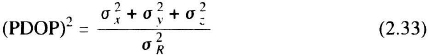
and ![]() in locally level coordinates, then, by definition, the position dilution of precision is
in locally level coordinates, then, by definition, the position dilution of precision is
and the horizontal dilution of precision (HDOP) is
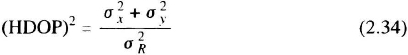
In pseudoranging systems, the GDOP is
(GDOP)2 = (PDOP)2 + (TDOP)2
where TDOP is the time dilution of precision, the contribution of clock error to the error in pseudorange. Equations for GDOP, PDOP, and HDOP, when the standard deviations in range to each station are different, are provided in [12]. Dilution of precision plays an important role in radio-ranging computations, especially for Loran (Chapter 4) and GPS (Chapter 5). Detailed GDOP equations for Loran are in Section 4.5.1, for Omega in Section 4.5.2, and for GPS in Section 5.5.2. Receivers usually flag a PDOP or HDOP greater than approximately 6 as an indication of poor geometry of the radio stations, hence a poor fix.
2.9 DIGITAL CHARTS
Traditional aeronautical charts are printed on paper. They are of three kinds:
- Visual charts. Showing terrain, airports, some navaids, restricted areas
- En-route instrument charts. Showing airways, navigation aids, intersections, restricted areas, and legal boundaries of controlled airspace. Airways are annotated to show altitude restrictions; high terrain is identified.
- Approach plates, standard approaches (STARs), and standard departures (SIDs). Showing horizontal and vertical profiles of preselected paths to and from the runway, beginning or ending at en-route fixes. High terrain and man-made obstacles are indicated. Missed approaches to a holding fix are described visually.
Military targeting charts show the expected location of defenses, the initial approach fix, the direction of approach, a visual picture of the target in season (e.g., snow covered) and the preplanned escape route.
Since World War II, experiments have been made with analog charts driven by automatic navigation equipment. Paper charts were unrolled or scanned onto CRTs, while an aircraft “bug” was driven by the navigation computations. The systems were limited by cost, reliability, and the need for wide swaths of chart to allow for diversion. Their use was confined to some helicopters and experimental military aircraft.
In 1996, digital maps were well-established in surveying data bases, the census, automotive navigation, and other specialized uses. Manufacturers of navigation sets created their own data base of navaids and airports or purchased one. Small digital data bases were included in the navaid's ROM whereas large data bases, especially those that included terrain, were usually delivered to customers on CD-ROM. National cartographic services in the developed world were all converting from paper maps to digital data bases. The U.S. Defense Mapping Agency (DMA) issued a standard for topographic maps on CD-ROM [19], and several other nations' cartographic agencies were doing the same. The U.S. Defense Mapping Agency produces separate data bases for terrain elevation and cultural features. They can be stored separately and superimposed on an airborne display. A U.S. National Imagery Transmission Format was created to send and store digital data. The GRASS language was widely used in the United States to manipulate DMA data [6]. Private companies were producing remarkably diverse Geographic Information System (GIS) data bases. In 1996, at least one company (Jeppesen) was producing digital approach plates on CD-ROM [4]. RTCA published a guide to aeronautical data bases [24a] as did ARINC [26a].
The technical challenges have been (1) to standardize the medium (e.g., CD-ROM), (2) to standardize the format of data stored on the medium so that any disc could be loaded onto any aircraft, just as any chart can be carried on any aircraft, and (3) to develop on-board software that displays sections of the chart across which the aircraft seems to move (moving map or moving bug, or both) and orient the chart properly (north up or velocity vector up). As the aircraft nears the edge of the chart, the software must move to a new section while avoiding hysteresis when flying near the edge of a chart. The expectation is that CD-ROM en-route and approach charts will be readily available to military users before the year 2000.
Digital chart displays have provisions for weather or terrain overlays (from airborne radar or from uplinked data), and provisions for traffic overlays (from on-board TCAS, ground uplink on Mode-S, or position broadcasts from other aircraft. Chapter 14). Civil airlines, driven by cost considerations, may gradually abandon their practice of purchasing charts and distributing them to the crews in hard copy. Instead, they may at first print charts on demand in the dispatch room from a central data base and, later, distribute portable digital charts on CD-ROM or via radio uplink to be loaded into the aircraft avionics when the crew boards.
2.10 SOFTWARE DEVELOPMENT
The sequence of activities in preparing the navigation software is as follows:
- The vehicle requirements are decomposed into the navigation system requirements. The navigation functions are allocated to hardware and software, usually after trade-off studies.
- A mathematical model of the vehicle and sensors is prepared. Sensors, such as radars and inertial instruments, are simulated with respect to accuracy and reliability.
- Engineering simulations are conducted on the accuracy model to determine the scaling, calculation speed, memory size, word length, and minimum degree of complexity required to obtain acceptable accuracy. Reference trajectories are defined, that specify flight paths, speed profiles, and attitude histories. Often man-in-the-loop simulations are required using a cockpit mock-up to assess the crew's work load. Another simulation determines the system's reliability and availability, given the known reliability of the constituent sensors and computers.
- The equations are coded for the flight computer. Prior to 1975, most navigation software was coded in assembly language to increase the execution speed. Thereafter, higher-order languages such as Fortran, C, Pascal, Jovial, and Ada have been used, though hardware drivers are often still written in assembly language. subroutines and functional modules come from libraries of well-tested routines that are re-used. The modules are individually tested; then the complete program is gradually compiled and tested. The contents must be documented at each stage, a process called configuration control.
- The code is verified by an independent agent. Mission-critical code, whose failure causes diversion of the aircraft, undergoes a simple verification, sometimes by engineers in the same company who did not participate in the development or test of the code. However, if navigation code is embedded with code that can cause loss of the aircraft (safety-critical code), the code must be further verified, usually by an independent organization using independently derived mathematical models of the aircraft and sensors. The high cost of independent verification encourages architectures in which safety-critical code is segregated. RTCA describes the certification of airborne software [24d] as does ARINC [26b].
- The code is loaded into ROM chips (often into ultraviolet-erasable EPROMs or into electrically-erasable programmable ROMs called EEPROMs or flash ROMs) that are installed in the computer by the manufacturer. EEPROM and flash-ROM code can be field-altered using test connectors. Sometimes, when navigation is not embedded into safety-critical software, the code is delivered to the airbase on tape or CD-ROM and loaded into the flight computer via the on-board data bus. Revisions of flight software may be issued from time to time.
- A copy of the flight software is usually delivered to a training facility, where it is used to check out crews in a ground simulator. The simulator may be a part-task computer-based trainer (CBT); a terminal that emulates the navigation keyboards, on-board computer, and displays; or it may be a high-fidelity emulation of the cockpit and avionics. A high-fidelity simulator may incorporate a flight computer that contains the navigation software or may rely on a scientific computer, programmed to emulate the flight computer. In a CBT, sensor inputs are simulated; in a high-fidelity simulator, they may come from real or simulated hardware. Simulator training is cheaper and often more effective than flight training.
- The final task in the preparation of the navigation software is the evaluation of its performance during flight versus the specification. This is done by the aircraft manufacturer or operator.
2.11 FUTURE TRENDS
The increasing capability of airborne digital computers will permit more complex algorithms to be solved. Companies that specialize in aircraft navigation will continue to build libraries of proprietary algorithms that they incorporate into their products. Crew interfaces will become more graphical to reduce workload and reduce errors in loading data. Direct loads from the ground via Mode-S links and other data links (some via satellite) will be commonplace.
By the year 2000, on-board CD-ROM readers will display charts and flight-manual data on military aircraft. The civil aviation industry may prefer to print up-to-date paper charts for each flight in the dispatch rooms, downloaded from a central data base, as an alternative to procuring and distributing them.
The software verification costs assigned to each aircraft will be substantial, because they are amortized over a few hundred units, even with standard libraries of routines.
PROBLEMS
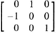
2.1. The direction cosine matrix [C] transforms the Earth-centered inertial coordinates yi into the locally-level navigation coordinates zj. Let α = 0 when the aircraft is on the equator, and let the initial matrix be

Let ![]() .
.
- (a) If the aircraft flies 90° due east, show the direction cosine matrix.

- (b) If the aircraft flies 90° due north from its original position, show the direction cosine matrix.
Ans:
- (c) If the aircraft flies 30° due east on the equator at 600 knots from its original position, what are the Cij and the
 ? Use Equation 7.40.
Ans:

2.2. An aircraft flies 3 hrs east then 2 hrs north at 300 knots at an altitude of 3 nmi, starting at 40° north latitude.
- (a) Find its position using the flat-Earth dead-reckoning equations.
Ans. x = 900 nmi, y = 600 nmi.
- (b) Find the final latitude-longitude using spherical-Earth equations with the Gaussian radius of curvature.
Ans. Φ = 49.98°, Δλ = 19.54°.
- (c) Find the final latitude-longitude using the ellipsoidal-Earth equations, (2.5).
Ans. Φ = 49.99°, Δλ = 19.50°.
- (d) Find the distance from the start to the destination of case a using the flat-Earth range equation, 2.20.
Ans. 1081.7 nmi.
- (e) Find the distance to the destination of case b using the spherical-Earth approximation with the Gaussian radius of curvature.
Ans. 1022.7 nmi.
- (f) Find the distance to the destination of case b using the flat-Earth equations plus the correction of Equation 2.21.
Ans. 1027.0 nmi.
2.3. A GPS satellite is at the ECEF coordinates:
![]()
The observer is at latitude 45°, longitude 45°, 30,000-ft altitude. Calculate the distance from the aircraft to the satellite and the elevation of the line of sight. Use the WGS dimensions on page 25.
Ans. R = 12,986.56 nmi, θ = 43.5 deg.
2.4. Derive Equation 2.21. Hint: solve the spherical triangle for the cosine of the range angle and express the coordinates of the waypoint as the present position plus a small increment. Expand the sines to third order and the cosines to second order.
2.5. Verify the calculations on page 46 for the probability of falling inside a rectangle of edge 1.2 nmi (x = 0.6 nmi) by 2.4 nmi (y = 1.2 nmi). Let σx = 0.4 nmi and σy = 2.4 nmi.