
Chapter 5. Overfitting and Its Avoidance
Fundamental concepts: Generalization; Fitting and overfitting; Complexity control.
Exemplary techniques: Cross-validation; Attribute selection; Tree pruning; Regularization.
One of the most important fundamental notions of data science is that of overfitting and generalization. If we allow ourselves enough flexibility in searching for patterns in a particular dataset, we will find patterns. Unfortunately, these “patterns” may be just chance occurrences in the data. As discussed previously, we are interested in patterns that generalize—that predict well for instances that we have not yet observed. Finding chance occurrences in data that look like interesting patterns, but which do not generalize, is called overfitting the data.
Generalization
Consider the following (extreme) example. You’re a manager at MegaTelCo, responsible for reducing customer churn. I run a data mining consulting group. You give my data science team a set of historical data on customers who have stayed with the company and customers who have departed within six months of contract expiration. My job is to build a model to distinguish customers who are likely to churn based on some features, as we’ve discussed previously. I mine the data and build a model. I give you back the code for the model, to implement in your company’s churn-reduction system.
Of course you are interested in whether my model is any good, so you ask your technical team to check the performance of the model on the historical data. You understand that historical performance is no guarantee of future success, but your experience tells you that churn patterns remain relatively stable, except for major changes to the industry (such as the introduction of the iPhone), and you know of no such major changes since these data were collected. So, the tech team runs the historical dataset through the model. Your technical lead reports back that this data science team is amazing. The model is 100% accurate. It does not make a single mistake, identifying correctly all the churners as well as the nonchurners.
You’re experienced enough not to be comfortable with that answer. You’ve had experts looking at churn behavior for a long time, and if there really were 100% accurate indicators, you figure you would be doing better than you currently are. Maybe this is just a lucky fluke?
It was not a lucky fluke. Our data science team can do that every time. Here is how we built the model. We stored the feature vector for each customer who has churned in a database table. Let’s call that Tc. Then, in use, when the model is presented with a customer to determine the likelihood of churning, it takes the customer’s feature vector, looks her up in Tc, and reports “100% likelihood of churning” if she is in Tc and “0% likelihood of churning” if she is not in Tc. So, when the tech team applies our model to the historical dataset, the model predicts perfectly.[28]
Call this simple approach a table model. It memorizes the training data and performs no generalization. What is the problem with this? Consider how we’ll use the model in practice. When a previously unseen customer’s contract is about to expire, we’ll want to apply the model. Of course, this customer was not part of the historical dataset, so the lookup will fail since there will be no exact match, and the model will predict “0% likelihood of churning” for this customer. In fact, the model will predict this for every customer (not in the training data). A model that looked perfect would be completely useless in practice!
This may seem like an absurd scenario. In reality, no one would throw raw customer data into a table and claim it was a “predictive model” of anything. But it is important to think about why this is a bad idea, because it fails for the same reason other, more realistic data mining efforts may fail. It is an extreme example of two related fundamental concepts of data science: generalization and overfitting. Generalization is the property of a model or modeling process, whereby the model applies to data that were not used to build the model. In this example, the model does not generalize at all beyond the data that were used to build it. It is tailored, or “fit,” perfectly to the training data. In fact, it is “overfit.”
This is the important point. Every dataset is a finite sample of a population—in this case, the population of phone customers. We want models to apply not just to the exact training set but to the general population from which the training data came. We may worry that the training data were not representative of the true population, but that is not the problem here. The data were representative, but the data mining did not create a model that generalized beyond the training data.
Overfitting
Overfitting is the tendency of data mining procedures to tailor models to the training data, at the expense of generalization to previously unseen data points. The example from the previous section was contrived; the data mining built a model using pure memorization, the most extreme overfitting procedure possible. However, all data mining procedures have the tendency to overfit to some extent—some more than others. The idea is that if we look hard enough we will find patterns in a dataset. As the Nobel Laureate Ronald Coase said, “If you torture the data long enough, it will confess.”
Unfortunately, the problem is insidious. The answer is not to use a data mining procedure that doesn’t overfit because all of them do. Nor is the answer to simply use models that produce less overfitting, because there is a fundamental trade-off between model complexity and the possibility of overfitting. Sometimes we may simply want more complex models, because they will better capture the real complexities of the application and thereby be more accurate. There is no single choice or procedure that will eliminate overfitting. The best strategy is to recognize overfitting and to manage complexity in a principled way.
The rest of this chapter discusses overfitting in more detail, methods for assessing the degree of overfitting at modeling time, as well as methods for avoiding overfitting as much as possible.
Overfitting Examined
Before discussing what to do about overfitting, we need to know how to recognize it.
Holdout Data and Fitting Graphs
Let’s now introduce a simple analytic tool: the fitting graph. A fitting graph shows the accuracy of a model as a function of complexity. To examine overfitting, we need to introduce a concept that is fundamental to evaluation in data science: holdout data.
The problem in the prior section was that the model was evaluated on the training data—exactly the same data that were used to build it. Evaluation on training data provides no assessment of how well the model generalizes to unseen cases. What we need to do is to “hold out” some data for which we know the value of the target variable, but which will not be used to build the model. These are not the actual use data, for which we ultimately would like to predict the value of the target variable. Instead, creating holdout data is like creating a “lab test” of generalization performance. We will simulate the use scenario on these holdout data: we will hide from the model (and possibly the modelers) the actual values for the target on the holdout data. The model will predict the values. Then we estimate the generalization performance by comparing the predicted values with the hidden true values. There is likely to be a difference between the model’s accuracy on the training set (sometimes called the “in-sample” accuracy) and the model’s generalization accuracy, as estimated on the holdout data. Thus, when the holdout data are used in this manner, they often are called the “test set.”
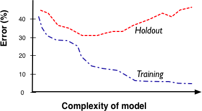
The accuracy of a model depends on how complex we allow it to be. A model can be complex in different ways, as we will discuss in this chapter. First let us use this distinction between training data and holdout data to define the fitting graph more precisely. The fitting graph (see Figure 5-1) shows the difference between a modeling procedure’s accuracy on the training data and the accuracy on holdout data as model complexity changes. Generally, there will be more overfitting as one allows the model to be more complex. (Technically, the chance of overfitting increases as one allows the modeling procedure more flexibility in the models it can produce; we will ignore that distinction in this book).
Figure 5-2 shows a fitting graph for the customer churn “table model” described earlier. Since this was an extreme example the fitting graph will be peculiar. Again, the x axis measures the complexity of the model; in this case, the number of rows allowed in the table. The y axis measures the error. As we allow the table to increase in size, we can memorize more and more of the training set, and with each new row the training set error decreases. Eventually the table is large enough to contain the entire training set (marked N on the x axis) and the error goes to zero and remains there. However, the testing (holdout) set error starts at some value (let’s call it b) and never decreases, because there is never an overlap between the training and holdout sets. The large gap between the two is a strong indication of memorization.

Note: Base rate
What would b be? Since the table model always predicts no churn for every
new case with which it is presented, it will get every no churn case right
and every churn case wrong. Thus the error rate will be the percentage of
churn cases in the population. This is known as the base rate, and a
classifier that always selects the majority class is called a base rate
classifier.
A corresponding baseline for a regression model is a simple model that always predicts the mean or median value of the target variable.
You will occasionally hear reference to “base rate performance,” and this is what it refers to. We will revisit the base rate again in the next chapter.
We’ve discussed in the previous chapters two very different sorts of modeling procedures: recursive partitioning of the data as done for tree induction, and fitting a numeric model by finding an optimal set of parameters, for example the weights in a linear model. We can now examine overfitting for each of these procedures.
Overfitting in Tree Induction
Recall how we built tree-structured models for classification. We applied a fundamental ability to find important, predictive individual attributes repeatedly (recursively) to smaller and smaller data subsets. Let’s assume for illustration that the dataset does not have two instances with exactly the same feature vector but different target values. If we continue to split the data, eventually the subsets will be pure—all instances in any chosen subset will have the same value for the target variable. These will be the leaves of our tree. There might be multiple instances at a leaf, all with the same value for the target variable. If we have to, we can keep splitting on attributes, and subdividing our data until we’re left with a single instance at each leaf node, which is pure by definition.
What have we just done? We’ve essentially built a version of the lookup table discussed in the prior section as an extreme example of overfitting! Any training instance given to the tree for classification will make its way down, eventually landing at the appropriate leaf—the leaf corresponding to the subset of the data that includes this particular training instance. What will be the accuracy of this tree on the training set? It will be perfectly accurate, predicting correctly the class for every training instance.
Will it generalize? Possibly. This tree should be slightly better than the lookup table because every previously unseen instance will arrive at some classification, rather than just failing to match; the tree will give a nontrivial classification even for instances it has not seen before. Therefore, it is useful to examine empirically how well the accuracy on the training data tends to correspond to the accuracy on test data.
A procedure that grows trees until the leaves are pure tends to overfit. Tree-structured models are very flexible in what they can represent. Indeed, they can represent any function of the features, and if allowed to grow without bound they can fit it to arbitrary precision. But the trees may need to be huge in order to do so. The complexity of the tree lies in the number of nodes.
Figure 5-3 shows a typical fitting graph for tree induction. Here we artificially limit the maximum size of each tree, as measured by the number of nodes it’s allowed to have, indicated on the x axis (which is log scale for convenience). For each tree size we create a new tree from scratch, using the training data. We measure two values: its accuracy on the training set and its accuracy on the holdout (test) set. If the data subsets at the leaves are not pure, we will predict the target variable based on some average over the target values in the subset, as we discussed in Chapter 3.
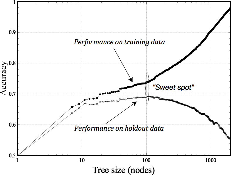
Beginning at the left, the tree is very small and has poor performance. As it is allowed more and more nodes it improves rapidly, and both training-set accuracy and holdout-set accuracy improve. Also we see that training-set accuracy always is at least a little better than holdout-set accuracy, since we did get to look at the training data when building the model. But at some point the tree starts to overfit: it acquires details of the training set that are not characteristic of the population in general, as represented by the holdout set. In this example overfitting starts to happen at around x = 100 nodes, denoted the “sweet spot” in the graph. As the trees are allowed to get larger, the training-set accuracy continues to increase—in fact, it is capable of memorizing the entire training set if we let it, leading to an accuracy of 1.0 (not shown). But the holdout accuracy declines as the tree grows past its “sweet spot”; the data subsets at the leaves get smaller and smaller, and the model generalizes from fewer and fewer data. Such inferences will be increasingly error-prone and the performance on the holdout data suffers.
In summary, from this fitting graph we may infer that overfitting on this dataset starts to dominate at around 100 nodes, so we should restrict tree size to this value.[29] This represents the best trade-off between the extremes of (i) not splitting the data at all and simply using the average target value in the entire dataset, and (ii) building a complete tree out until the leaves are pure.
Unfortunately, no one has come up with a procedure to determine this exact sweet spot theoretically, so we have to rely on empirically based techniques. Before discussing those, let’s examine overfitting in our second sort of modeling procedure.
Overfitting in Mathematical Functions
There are different ways to allow more or less complexity in mathematical functions. There are entire books on the topic. This section discusses one very important way, and * Avoiding Overfitting for Parameter Optimization discusses a second one. We urge you to at least skim that advanced (starred) section because it introduces concepts and vocabulary in common use by data scientists these days, that can make a non-data scientist’s head swim. Here we will summarize and give you enough to understand such discussions at a conceptual level.[30] But first, let’s discuss a much more straightforward way in which functions can become too complex.
One way mathematical functions can become more complex is by adding more variables (more attributes). For example, say that we have a linear model as described in Equation 4-2:

As we add more xi’s, the function becomes more and more complicated. Each xi has a corresponding wi, which is a learned parameter of the model.
Modelers sometimes even change the function from being truly linear in the original attributes by adding new attributes that are nonlinear versions of original attributes. For example, I might add a fourth attribute x4=x12. Also, we might expect that the ratio of x2 and x3 is important, so we add a new attribute x5 = x2/x3. Now we’re trying to find the parameters (weights) of:

Either way, a dataset may end up with a very large number of attributes, and using all of them gives the modeling procedure much leeway to fit the training set. You might recall from geometry that in two dimensions you can fit a line to any two points and in three dimensions you can fit a plane to any three points. This concept generalizes: as you increase the dimensionality, you can perfectly fit larger and larger sets of arbitrary points. And even if you cannot fit the dataset perfectly, you can fit it better and better with more dimensions—that is, with more attributes.
Often, modelers carefully prune the attributes in order to avoid overfitting. Modelers will use a sort of holdout technique introduced above to assess the information in the individual attributes. Careful manual attribute selection is a wise practice in cases where considerable human effort can be spent on modeling, and where there are reasonably few attributes. In many modern applications, where large numbers of models are built automatically, and/or where there are very large sets of attributes, manual selection may not be feasible. For example, companies that do data science-driven targeting of online display advertisements can build thousands of models each week, sometimes with millions of possible features. In such cases there is no choice but to employ automatic feature selection (or to ignore feature selection all together).
Example: Overfitting Linear Functions
In An Example of Mining a Linear Discriminant from Data, we introduced a simple dataset called iris, comprising data describing two species of Iris flowers. Now let’s revisit that to see the effects of overfitting in action.
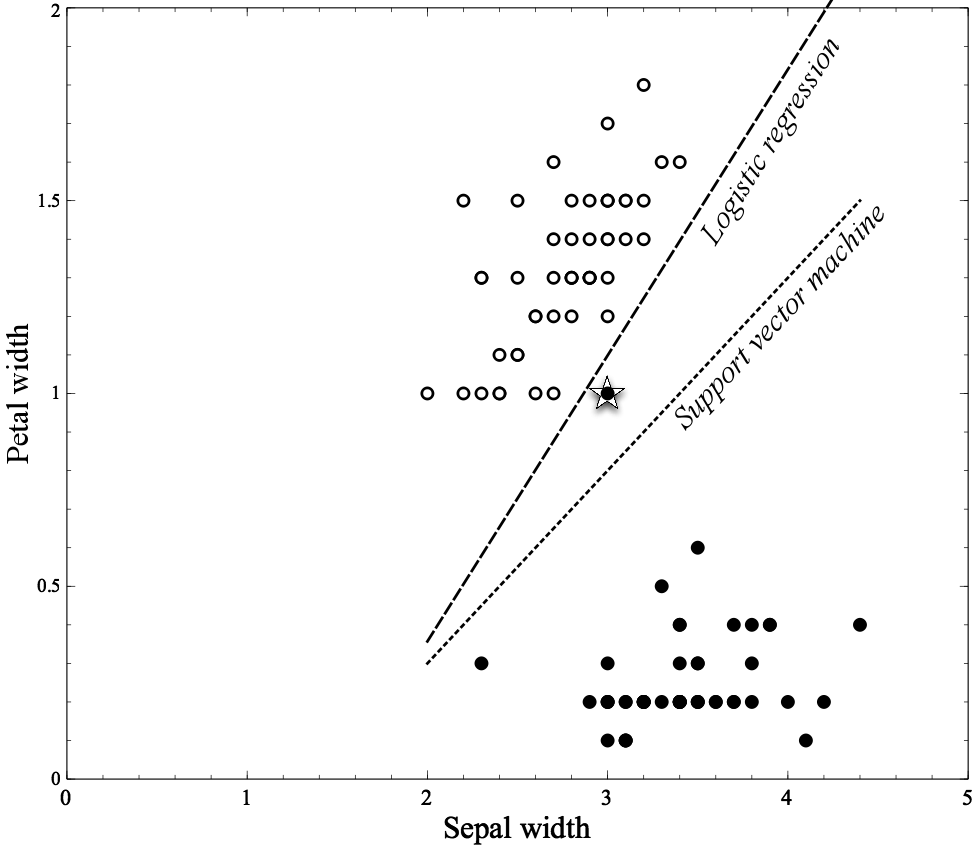
Figure 5-4 shows the original Iris dataset graphed with its two attributes, Petal width and Sepal width. Recall that each instance is one flower and corresponds to one dot on the graph. The filled dots are of the species Iris Setosa and the circles are instances of the species Iris Versicolor. Note several things here: first, the two classes of iris are very distinct and separable. In fact, there is a wide gap between the two “clumps” of instances. Both logistic regression and support vector machines place separating boundaries (lines) in the middle. In fact, the two separating lines are so similar that they’re indistinguishable in the graph.

In Figure 5-5, we’ve added a single new example: an Iris Setosa point at (3,1). Realistically, we might consider this example to be an outlier or an error since it’s much closer to the Versicolor examples than the Setosas. Notice how the logistic regression line moves in response: it separates the two groups perfectly, while the SVM line barely moves at all.
In Figure 5-6 we’ve added a different outlier at (4,0.7), this time a Versicolor example down in the Setosa region. Again, the support vector machine line moves very little in response, but the logistic regression line moves considerably.
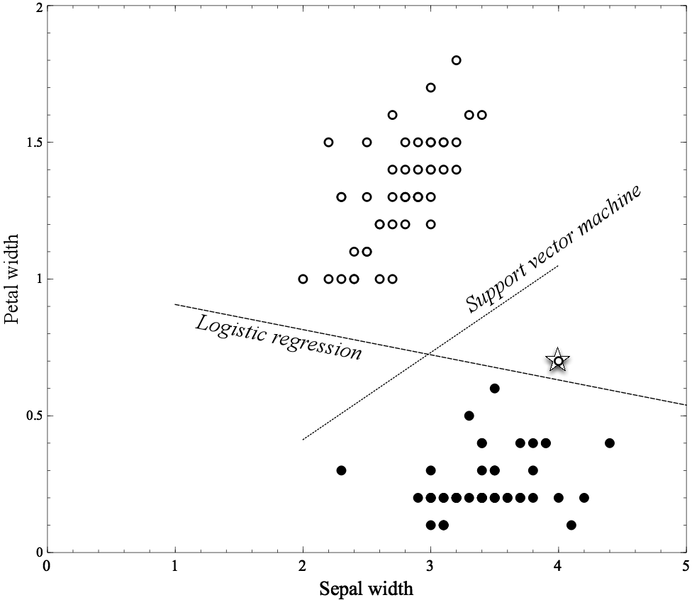
In Figure 5-5 and Figure 5-6, Logistic regression appears to be overfitting. Arguably, the examples introduced in each are outliers that should not have a strong influence on the model—they contribute little to the “mass” of the species examples. Yet in the case of logistic regression they clearly do. If a linear boundary exists, logistic regression will find it,[31] even if this means moving the boundary to accommodate outliers. The SVM tends to be less sensitive to individual examples. The SVM training procedure incorporates complexity control, which we will describe technically later.

As we said earlier, another way mathematical functions can become more complex is by adding more variables. In Figure 5-7, we have done just this: we used the same dataset as in Figure 5-6 but we added a single extra attribute, the square of the Sepal width. Providing this attribute gives each method more flexibility in fitting the data because it may assign weights to the squared term. Geometrically, this means the separating boundary can be not just a line but a parabola. This additional freedom allows both methods to create curved surfaces that can fit the regions more closely. In cases where curved surfaces may be necessary, this freedom may be necessary, but it also gives the methods far more opportunity to overfit. Note however that the SVM, even though its boundary now is curved, the training procedure still has opted for the larger margin around the boundary, rather than the perfect separation of the positive different classes.
* Example: Why Is Overfitting Bad?
Technical Details Ahead
At the beginning of the chapter, we said that a model that only memorizes is useless because it always overfits and is incapable of generalizing. But technically this only demonstrates that overfitting hinders us from improving a model after a certain complexity. It does not explain why overfitting often causes models to become worse, as Figure 5-3 shows. This section goes into a detailed example showing how this happens and why. It may be skipped without loss of continuity.
Why does performance degrade? The short answer is that as a model gets more complex it is allowed to pick up harmful spurious correlations. These correlations are idiosyncrasies of the specific training set used and do not represent characteristics of the population in general. The harm occurs when these spurious correlations produce incorrect generalizations in the model. This is what causes performance to decline when overfitting occurs. In this section we go through an example in detail to show how this can happen.
Consider a simple two-class problem with classes c1 and c2 and attributes x and y. We have a population of examples, evenly balanced between the classes. Attribute x has two values, p and q, and y has two values, r and s. In the general population, x = p occurs 75% of the time in class c1 examples and in 25% of the c2 examples, so x provides some prediction of the class. By design, y has no predictive power at all, and indeed we see that in the data sample both of y’s values occur in both classes equally. In short, the instances in this domain are difficult to separate, with only x providing some predictive power. The best we can achieve is 75% accuracy by looking at x.

Table 5-1 shows a very small training set of examples from this domain. What would a classification tree learner do with these? We won’t go into the entropy calculations, but attribute x provides some leverage so a tree learner would split on it and create the tree shown in Figure 5-8. Since x provides the only leverage, this should be the optimal tree. Its error rate is 25%—equal to the theoretical minimum error rate.
However, observe from Table 5-1 that in this particular dataset y’s values of r and s are not evenly split between the classes, so y does seem to provide some predictiveness. Specifically, once we choose x=p (instances 1-4), we see that y=r predicts c1 perfectly (instances 1-3). Hence, from this dataset, tree induction would achieve information gain by splitting on y’s values and create two new leaf nodes, shown in Figure 5-8.
Based on our training set, the tree in (b) performs well, better than (a). It classifies seven of the eight training examples correctly, whereas the tree in (a) classifies only six out of eight correct. But this is due to the fact that y=r purely by chance correlates with class c1 in this data sample; in the general population there is no such correlation. We have been misled, and the extra branch in (b) is not simply extraneous, it is harmful. Recall that we defined the general population to have x=p occurring in 75% of the class c1 examples and 25% of the c2 examples. But the spurious y=s branch predicts c2, which is wrong in the general population. In fact, we expect this spurious branch to contribute one in eight errors made by the tree. Overall, the (b) tree will have a total expected error rate of 30%, while (a) will have an error rate of 25%.
We conclude this example by emphasizing several points. First, this phenomenon is not particular to classification trees. Trees are convenient for this example because it is easy to point to a portion of a tree and declare it to be spurious, but all model types are susceptible to overfitting effects. Second, this phenomenon is not due to the training data in Table 5-1 being atypical or biased. Every dataset is a finite sample of a larger population, and every sample will have variations even when there is no bias in the sampling. Finally, as we have said before, there is no general analytic way to determine in advance whether a model has overfit or not. In this example we defined what the population looked like so we could declare that a given model had overfit. In practice, you will not have such knowledge and it will be necessary to use a holdout set to detect overfitting.
From Holdout Evaluation to Cross-Validation
Later we will present a general technique in broad use to try to avoid overfitting, which applies to attribute selection as well as tree complexity, and beyond. But first, we need to discuss holdout evaluation in more detail. Before we can work to avoid overfitting, we need to be able to avoid being fooled by overfitting. At the beginning of this chapter we introduced the idea that in order to have a fair evaluation of the generalization performance of a model, we should estimate its accuracy on holdout data—data not used in building the model, but for which we do know the actual value of the target variable. Holdout testing is similar to other sorts of evaluation in a “laboratory” setting.
While a holdout set will indeed give us an estimate of generalization performance, it is just a single estimate. Should we have any confidence in a single estimate of model accuracy? It might have just been a single particularly lucky (or unlucky) choice of training and test data. We will not go into the details of computing confidence intervals on such quantities, but it is important to discuss a general testing procedure that will end up helping in several ways.
Cross-validation is a more sophisticated holdout training and testing procedure. We would like not only a simple estimate of the generalization performance, but also some statistics on the estimated performance, such as the mean and variance, so that we can understand how the performance is expected to vary across datasets. This variance is critical for assessing confidence in the performance estimate, as you might have learned in a statistics class.
Cross-validation also makes better use of a limited dataset. Unlike splitting the data into one training and one holdout set, cross-validation computes its estimates over all the data by performing multiple splits and systematically swapping out samples for testing.
Cross-validation begins by splitting a labeled dataset into k partitions called folds. Typically, k will be five or ten. The top pane of Figure 5-9 shows a labeled dataset (the original dataset) split into five folds. Cross-validation then iterates training and testing k times, in a particular way. As depicted in the bottom pane of Figure 5-9, in each iteration of the cross-validation, a different fold is chosen as the test data. In this iteration, the other k–1 folds are combined to form the training data. So, in each iteration we have (k–1)/k of the data used for training and 1/k used for testing.
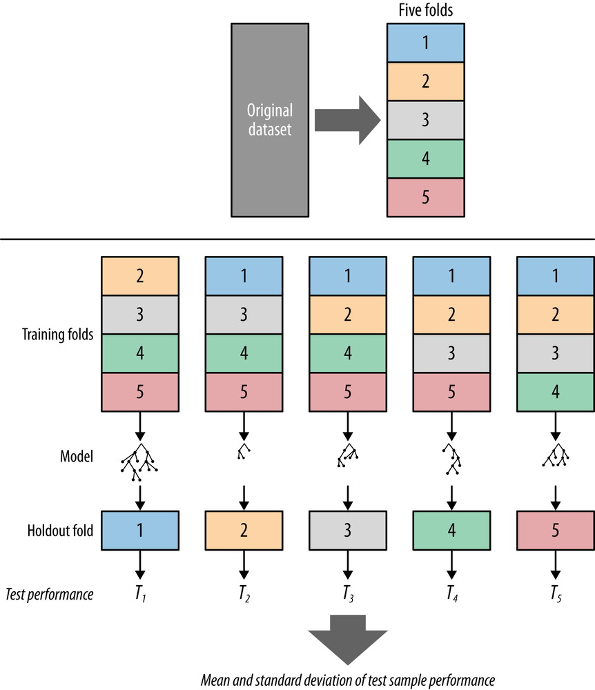
Each iteration produces one model, and thereby one estimate of generalization performance, for example, one estimate of accuracy. When cross-validation is finished, every example will have been used only once for testing but k–1 times for training. At this point we have performance estimates from all the k folds and we can compute the average and standard deviation.
The Churn Dataset Revisited
Consider again the churn dataset introduced in Example: Addressing the Churn Problem with Tree Induction. In that section we used the entire dataset both for training and testing, and we reported an accuracy of 73%. We ended that section by asking a question, Do you trust this number? By this point you should know enough to mistrust any performance measurement done on the training set, because overfitting is a very real possibility. Now that we have introduced cross-validation we can redo the evaluation more carefully.
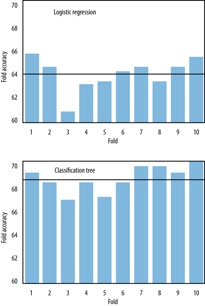
Figure 5-10 shows the results of ten-fold cross-validation. In fact, two model types are shown. The top graph shows results with logistic regression, and the bottom graph shows results with classification trees. To be precise: the dataset was first shuffled, then divided into ten partitions. Each partition in turn served as a single holdout set while the other nine were collectively used for training. The horizontal line in each graph is the average of accuracies of the ten models of that type.
There are several things to observe here. First, the average accuracy of the folds with classification trees is 68.6%—significantly lower than our previous measurement of 73%. This means there was some overfitting occurring with the classification trees, and this new (lower) number is a more realistic measure of what we can expect. Second, there is variation in the performances in the different folds (the standard deviation of the fold accuracies is 1.1), and thus it is a good idea to average them to get a notion of the performance as well as the variation we can expect from inducing classification trees on this dataset.
Finally, compare the fold accuracies between logistic regression and classification trees. There are certain commonalities in both graphs—for example, neither model type did very well on Fold Three and both performed well on Fold Ten. But there are definite differences between the two. An important thing to notice is that logistic regression models show slightly lower average accuracy (64.1%) and with higher variation (standard deviation of 1.3) than the classification trees do. On this particular dataset, trees may be preferable to logistic regression because of their greater stability and performance. But this is not absolute; other datasets will produce different results, as we shall see.
Learning Curves
If the training set size changes, you may also expect different generalization performance from the resultant model. All else being equal, the generalization performance of data-driven modeling generally improves as more training data become available, up to a point. A plot of the generalization performance against the amount of training data is called a learning curve. The learning curve is another important analytical tool.
Learning curves for tree induction and logistic regression are shown in Figure 5-11 for the telecommunications churn problem.[32] Learning curves usually have a characteristic shape. They are steep initially as the modeling procedure finds the most apparent regularities in the dataset. Then as the modeling procedure is allowed to train on larger and larger datasets, it finds more accurate models. However, the marginal advantage of having more data decreases, so the learning curve becomes less steep. In some cases, the curve flattens out completely because the procedure can no longer improve accuracy even with more training data.
It is important to understand the difference between learning curves and fitting graphs (or fitting curves). A learning curve shows the generalization performance—the performance only on testing data, plotted against the amount of training data used. A fitting graph shows the generalization performance as well as the performance on the training data, but plotted against model complexity. Fitting graphs generally are shown for a fixed amount of training data.
Even on the same data, different modeling procedures can produce very different learning curves. In Figure 5-11, observe that for smaller training-set sizes, logistic regression yields better generalization accuracy than tree induction. However, as the training sets get larger, the learning curve for logistic regression levels off faster, the curves cross, and tree induction soon is more accurate. This performance relates back to the fact that with more flexibility comes more overfitting. Given the same set of features, classification trees are a more flexible model representation than linear logistic regression. This means two things: for smaller data, tree induction will tend to overfit more. Often, as we see for the data in Figure 5-11, this leads logistic regression to perform better for smaller datasets (not always, though). On the other hand, the figure also shows that the flexibility of tree induction can be an advantage with larger training sets: the tree can represent substantially nonlinear relationships between the features and the target. Whether the tree induction can actually capture those relationships needs to be evaluated empirically—using an analytical tool such as learning curves.

Note
The learning curve has additional analytical uses. For example, we’ve made the point that data can be an asset. The learning curve may show that generalization performance has leveled off so investing in more training data is probably not worthwhile; instead, one should accept the current performance or look for another way to improve the model, such as by devising better features. Alternatively, the learning curve might show generalization accuracy continuing to improve, so obtaining more training data could be a good investment.
Overfitting Avoidance and Complexity Control
To avoid overfitting, we control the complexity of the models induced from the data. Let’s start by examining complexity control in tree induction, since tree induction has much flexibility and therefore will tend to overfit a good deal without some mechanism to avoid it. This discussion in the context of trees will lead us to a very general mechanism that will be applicable to other models.
Avoiding Overfitting with Tree Induction
The main problem with tree induction is that it will keep growing the tree to fit the training data until it creates pure leaf nodes. This will likely result in large, overly complex trees that overfit the data. We have seen how this can be detrimental. Tree induction commonly uses two techniques to avoid overfitting. These strategies are (i) to stop growing the tree before it gets too complex, and (ii) to grow the tree until it is too large, then “prune” it back, reducing its size (and thereby its complexity).
There are various methods for accomplishing both. The simplest method to limit tree size is to specify a minimum number of instances that must be present in a leaf. The idea behind this minimum-instance stopping criterion is that for predictive modeling, we essentially are using the data at the leaf to make a statistical estimate of the value of the target variable for future cases that would fall to that leaf. If we make predictions of the target based on a very small subset of data, we might expect them to be inaccurate—especially when we built the tree specifically to try to get pure leaves. A nice property of controlling complexity in this way is that tree induction will automatically grow the tree branches that have a lot of data and cut short branches that have fewer data—thereby automatically adapting the model based on the data distribution.
A key question becomes what threshold we should use. How few instances are we willing to tolerate at a leaf? Five instances? Thirty? One hundred? There is no fixed number, although practitioners tend to have their own preferences based on experience. However, researchers have developed techniques to decide the stopping point statistically. Statistics provides the notion of a “hypothesis test,” which you might recall from a basic statistics class. Roughly, a hypothesis test tries to assess whether a difference in some statistic is not due simply to chance. In most cases, the hypothesis test is based on a “p-value,” which gives a limit on the probability that the difference in statistic is due to chance. If this value is below a threshold (often 5%, but problem specific), then the hypothesis test concludes that the difference is likely not due to chance. So, for stopping tree growth, an alternative to setting a fixed size for the leaves is to conduct a hypothesis test at every leaf to determine whether the observed difference in (say) information gain could have been due to chance. If the hypothesis test concludes that it was likely not due to chance, then the split is accepted and the tree growing continues. (See Sidebar: Beware of “multiple comparisons”.)
The second strategy for reducing overfitting is to “prune” an overly large tree. Pruning means to cut off leaves and branches, replacing them with leaves. There are many ways to do this, and the interested reader can look into the data mining literature for details. One general idea is to estimate whether replacing a set of leaves or a branch with a leaf would reduce accuracy. If not, then go ahead and prune. The process can be iterated on progressive subtrees until any removal or replacement would reduce accuracy.
We conclude our example of avoiding overfitting in tree induction with the method that will generalize to many different data modeling techniques. Consider the following idea: what if we built trees with all sorts of different complexities? For example, say we stop building the tree after only one node. Then build a tree with two nodes. Then three nodes, etc. We have a set of trees of different complexities. Now, if only there were a way to estimate their generalization performance, we could pick the one that is (estimated to be) the best!
A General Method for Avoiding Overfitting
More generally, if we have a collection of models with different complexities, we could choose the best simply by estimating the generalization performance of each. But how could we estimate their generalization performance? On the (labeled) test data? There’s one big problem with that: test data should be strictly independent of model building so that we can get an independent estimate of model accuracy. For example, we might want to estimate the ultimate business performance or to compare the best model we can build from one family (say, classification trees) against the best model from another family (say, logistic regression). If we don’t care about comparing models or getting an independent estimate of the model accuracy and/or variance, then we could pick the best model based on the testing data.
However, even if we do want these things, we still can proceed. The key is to realize that there was nothing special about the first training/test split we made. Let’s say we are saving the test set for a final assessment. We can take the training set and split it again into a training subset and a testing subset. Then we can build models on this training subset and pick the best model based on this testing subset. Let’s call the former the sub-training set and the latter the validation set for clarity. The validation set is separate from the final test set, on which we are never going to make any modeling decisions. This procedure is often called nested holdout testing.
Returning to our classification tree example, we can induce trees of many complexities from the subtraining set, then we can estimate the generalization performance for each from the validation set. This would correspond to choosing the top of the inverted-U-shaped holdout curve in Figure 5-3. Say the best model by this assessment has a complexity of 122 nodes (the “sweet spot”). Then we could use this model as our best choice, possibly estimating the actual generalization performance on the final holdout test set. We also could add one more twist. This model was built on a subset of our training data, since we had to hold out the validation set in order to choose the complexity. But once we’ve chosen the complexity, why not induce a new tree with 122 nodes from the whole, original training set? Then we might get the best of both worlds: using the subtraining/validation split to pick the best complexity without tainting the test set, and building a model of this best complexity on the entire training set (subtraining plus validation).
This approach is used in many sorts of modeling algorithms to control complexity. The general method is to choose the value for some complexity parameter by using some sort of nested holdout procedure. Again, it is nested because a second holdout procedure is performed on the training set selected by the first holdout procedure.
Often, nested cross-validation is used. Nested cross-validation is more complicated, but it works as you might suspect. Say we would like to do cross-validation to assess the generalization accuracy of a new modeling technique, which has an adjustable complexity parameter C, but we do not know how to set it. So, we run cross-validation as described above. However, before building the model for each fold, we take the training set (refer to Figure 5-9) and first run an experiment: we run another entire cross-validation on just that training set to find the value of C estimated to give the best accuracy. The result of that experiment is used only to set the value of C to build the actual model for that fold of the cross-validation. Then we build another model using the entire training fold, using that value for C, and test on the corresponding test fold. The only difference from regular cross-validation is that for each fold we first run this experiment to find C, using another, smaller, cross-validation.
If you understood all that, you would realize that if we used 5-fold cross-validation in both cases, we actually have built 30 total models in the process (yes, thirty). This sort of experimental complexity-controlled modeling only gained broad practical application over the last decade or so, because of the obvious computational burden involved.
This idea of using the data to choose the complexity experimentally, as well as to build the resulting model, applies across different induction algorithms and different sorts of complexity. For example, we mentioned that complexity increases with the size of the feature set, so it is usually desirable to cull the feature set. A common method for doing this is to run with many different feature sets, using this sort of nested holdout procedure to pick the best.
For example, sequential forward selection (SFS) of features uses a nested holdout procedure to first pick the best individual feature, by looking at all models built using just one feature. After choosing a first feature, SFS tests all models that add a second feature to this first chosen feature. The best pair is then selected. Next the same procedure is done for three, then four, and so on. When adding a feature does not improve classification accuracy on the validation data, the SFS process stops. (There is a similar procedure called sequential backward elimination of features. As you might guess, it works by starting with all features and discarding features one at a time. It continues to discard features as long as there is no performance loss.)
This is a common approach. In modern environments with plentiful data and computational power, the data scientist routinely sets modeling parameters by experimenting using some tactical, nested holdout testing (often nested cross-validation).
The next section shows a different way that this method applies to controlling overfitting when learning numerical functions (as described in Chapter 4). We urge you to at least skim the following section because it introduces concepts and vocabulary in common use by data scientists these days.
* Avoiding Overfitting for Parameter Optimization
As just described, avoiding overfitting involves complexity control: finding the “right” balance between the fit to the data and the complexity of the model. In trees we saw various ways for trying to keep the tree from getting too big (too complex) when fitting the data. For equations, such as logistic regression, that unlike trees do not automatically select what attributes to include, complexity can be controlled by choosing a “right” set of attributes.
Chapter 4 introduced the popular family of methods that builds models by explicitly optimizing the fit to the data via a set of numerical parameters. We discussed various linear members of this family, including linear discriminant learners, linear regression, and logistic regression. Many nonlinear models are fit to the data in exactly the same way.
As might be expected given our discussion so far in this chapter and the figures in Example: Overfitting Linear Functions, these procedures also can overfit the data. However, their explicit optimization framework provides an elegant, if technical, method for complexity control. The general strategy is that instead of just optimizing the fit to the data, we optimize some combination of fit and simplicity. Models will be better if they fit the data better, but they also will be better if they are simpler. This general methodology is called regularization, a term that is heard often in data science discussions.
Technical Details Ahead
The rest of this section discusses briefly (and slightly technically) how regularization is done. Don’t worry if you don’t really understand the technical details. Do remember that regularization is trying to optimize not just the fit to the data, but a combination of fit to the data and simplicity of the model.
Recall from Chapter 4 that to fit a model involving numeric parameters w to the data we find the set of parameters that maximizes some “objective function” indicating how well it fits the data:

(The arg maxw just means that you want to maximize the fit over all possible arguments w, and are interested in the particular argument w that gives the maximum. These would be the parameters of the final model.)
Complexity control via regularization works by adding to this objective function a penalty for complexity:

The λ term is simply a weight that determines how much importance the optimization procedure should place on the penalty, compared to the data fit. At this point, the modeler has to choose λ and the penalty function.
So, as a concrete example, recall from * Logistic Regression: Some Technical Details that to learn a standard logistic regression model, from data, we find the numeric parameters w that yield the linear model most likely to have generated the observed data—the “maximum likelihood” model. Let’s represent that as:
To learn a “regularized” logistic regression model we would instead compute:

There are different penalties that can be applied, with different properties.[33] The most commonly used penalty is the sum of the squares of the weights, sometimes called the “L2-norm” of w. The reason is technical, but basically functions can fit data better if they are allowed to have very large positive and negative weights. The sum of the squares of the weights gives a large penalty when weights have large absolute values.
If we incorporate the L2-norm penalty into standard least-squares linear regression, we get the statistical procedure called ridge regression. If instead we use the sum of the absolute values (rather than the squares), known as the L1-norm, we get a procedure known as the lasso (Hastie et al., 2009). More generally, this is called L1-regularization. For reasons that are quite technical, L1-regularization ends up zeroing out many coefficients. Since these coefficients are the multiplicative weights on the features, L1-regularization effectively performs an automatic form of feature selection.
Now we have the machinery to describe in more detail the linear support vector machine, introduced in Support Vector Machines, Briefly. There we waved our hands and told you that the support vector machine “maximizes the margin” between the classes by fitting the “fattest bar” between the classes. Separately we discussed that it uses hinge loss (see Sidebar: Loss functions) to penalize errors. We now can connect these together, and directly to logistic regression. Specifically, linear support vector machine learning is almost equivalent to the L2-regularized logistic regression just discussed; the only difference is that a support vector machine uses hinge loss instead of likelihood in its optimization. The support vector machine optimizes this equation:

where ghinge, the hinge loss term, is negated because lower hinge loss is better.
Finally, you may be saying to yourself: all this is well and good, but a lot of magic seems to be hidden in this λ parameter, which the modeler has to choose. How in the world would the modeler choose that for some real domain like churn prediction, or online ad targeting, or fraud detection?
It turns out that we already have a straightforward way to choose λ. We’ve discussed how a good tree size and a good feature set can be chosen via nested cross-validation on the training data. We can choose λ the same way. This cross-validation would essentially conduct automated experiments on subsets of the training data and find a good λ value. Then this λ would be used to learn a regularized model on all the training data. This has become the standard procedure for building numerical models that give a good balance between data fit and model complexity. This general approach to optimizing the parameter values of a data mining procedure is known as grid search.
Summary
Data mining involves a fundamental trade-off between model complexity and the possibility of overfitting. A complex model may be necessary if the phenomenon producing the data is itself complex, but complex models run the risk of overfitting training data (i.e., modeling details of the data that are not found in the general population). An overfit model will not generalize to other data well, even if they are from the same population.
All model types can be overfit. There is no single choice or technique to eliminate overfitting. The best strategy is to recognize overfitting by testing with a holdout set. Several types of curves can help detect and measure overfitting. A fitting graph has two curves showing the model performance on the training and testing data as a function of model complexity. A fitting curve on testing data usually has an approximate U or inverted-U-shape (depending on whether error or accuracy is plotted). The accuracy starts off low when the model is simple, increases as complexity increases, flattens out, then starts to decrease again as overfitting sets in. A learning curve shows model performance on testing data plotted against the amount of training data used. Usually model performance increases with the amount of data, but the rate of increase and the final asymptotic performance can be quite different between models.
A common experimental methodology called cross-validation specifies a systematic way of splitting up a single dataset such that it generates multiple performance measures. These values tell the data scientist what average behavior the model yields as well as the variation to expect.
The general method for reining in model complexity to avoid overfitting is called model regularization. Techniques include tree pruning (cutting a classification tree back when it has become too large), feature selection, and employing explicit complexity penalties into the objective function used for modeling.
[28] Technically, this is not necessarily true: there may be two customers with the same feature vector description, one of whom churns and the other does not. We can ignore that possibility for the sake of this example. For example, we can assume that the unique customer ID is one of the features.
[29] Note that 100 nodes is not some special universal value. It is specific to this particular dataset. If we changed the data significantly, or even just used a different tree-building algorithm, we’d probably want to make another fitting graph to find the new sweet spot.
[30] We also will have enough of a conceptual toolkit by that point to understand support vector machines a little better—as being almost equivalent to logistic regression with complexity (overfitting) control.
[31] Technically, only some logistic regression algorithms are guaranteed to find it. Some do not have this guarantee. However, this fact is not germane to the overfitting point we’re making here.
[32] Perlich et al. (2003) show learning curves for tree induction and logistic regression for dozens of classification problems.
[33] The book The Elements of Statistical Learning (Hastie, Tibshirani, & Friedman, 2009) contains an excellent technical discussion of these.