Chapter 10. Representing and Mining Text
Fundamental concepts: The importance of constructing mining-friendly data representations; Representation of text for data mining.
Exemplary techniques: Bag of words representation; TFIDF calculation; N-grams; Stemming; Named entity extraction; Topic models.
Up to this point we’ve ignored or side-stepped an important stage of the data mining process: data preparation. The world does not always present us with data in the feature vector representation that most data mining methods take as input. Data are represented in ways natural to problems from which they were derived. If we want to apply the many data mining tools that we have at our disposal, we must either engineer the data representation to match the tools, or build new tools to match the data. Top-notch data scientists employ both of these strategies. It generally is simpler to first try to engineer the data to match existing tools, since they are well understood and numerous.
In this chapter, we will focus on one particular sort of data that has become extremely common as the Internet has become a ubiquitous channel of communication: text data. Examining text data allows us to illustrate many real complexities of data engineering, and also helps us to understand better a very important type of data. We will see in Chapter 14 that although in this chapter we focus exclusively on text data, the fundamental principles indeed generalize to other important sorts of data.
We’ve encountered text once before in this book, in the example involving clustering news stories about Apple Inc. (Example: Clustering Business News Stories). There we deliberately avoided a detailed discussion of how the news stories were prepared because the focus was on clustering, and text preparation would have been too much of a digression. This chapter is devoted to the difficulties and opportunities of dealing with text.
In principle, text is just another form of data, and text processing is just a special case of representation engineering. In reality, dealing with text requires dedicated pre-processing steps and sometimes specific expertise on the part of the data science team. Entire books and conferences (and companies) are devoted to text mining. In this chapter we can only scratch the surface, to give a basic overview of the techniques and issues involved in typical business applications.
First, let’s discuss why text is so important and why it’s difficult.
Why Text Is Important
Text is everywhere. Many legacy applications still produce or record text. Medical records, consumer complaint logs, product inquiries, and repair records are still mostly intended as communication between people, not computers, so they’re still “coded” as text. Exploiting this vast amount of data requires converting it to a meaningful form.
The Internet may be the home of “new media,” but much of it is the same form as old media. It contains a vast amount of text in the form of personal web pages, Twitter feeds, email, Facebook status updates, product descriptions, Reddit comments, blog postings—the list goes on. Underlying the search engines (Google and Bing) that we use everyday are massive amounts of text-oriented data science. Music and video may account for a great deal of traffic volume, but when people communicate with each other on the Internet it is usually via text. Indeed, the thrust of Web 2.0 was about Internet sites allowing users to interact with one another as a community, and to generate much added content of a site. This user-generated content and interaction usually takes the form of text.
In business, understanding customer feedback often requires understanding text. This isn’t always the case; admittedly, some important consumer attitudes are represented explicitly as data or can be inferred through behavior, for example via five-star ratings, click-through patterns, conversion rates, and so on. We can also pay to have data collected and quantified through focus groups and online surveys. But in many cases if we want to “listen to the customer” we’ll actually have to read what she’s written—in product reviews, customer feedback forms, opinion pieces, and email messages.
Why Text Is Difficult
Text is often referred to as “unstructured” data. This refers to the fact that text does not have the sort of structure that we normally expect for data: tables of records with fields having fixed meanings (essentially, collections of feature vectors), as well as links between the tables. Text of course has plenty of structure, but it is linguistic structure—intended for human consumption, not for computers.
Words can have varying lengths and text fields can have varying numbers of words. Sometimes word order matters, sometimes not.
As data, text is relatively dirty. People write ungrammatically, they misspell words, they run words together, they abbreviate unpredictably, and punctuate randomly. Even when text is flawlessly expressed it may contain synonyms (multiple words with the same meaning) and homographs (one spelling shared among multiple words with different meanings). Terminology and abbreviations in one domain might be meaningless in another domain—we shouldn’t expect that medical recordkeeping and computer repair records would share terms in common, and in the worst case they would conflict.
Because text is intended for communication between people, context is important, much more so than with other forms of data. Consider this movie review excerpt:
“The first part of this movie is far better than the second. The acting is poor and it gets out-of-control by the end, with the violence overdone and an incredible ending, but it’s still fun to watch.”
Consider whether the overall sentiment is for or against the film. Is the word incredible positive or negative? It is difficult to evaluate any particular word or phrase here without taking into account the entire context.
For these reasons, text must undergo a good amount of preprocessing before it can be used as input to a data mining algorithm. Usually the more complex the featurization, the more aspects of the text problem can be included. This chapter can only describe some of the basic methods involved in preparing text for data mining. The next few subsections describe these steps.
Representation
Having discussed how difficult text can be, let’s go through the basic steps to transform a body of text into a set of data that can be fed into a data mining algorithm. The general strategy in text mining is to use the simplest (least expensive) technique that works. Nevertheless, these ideas are the key technology underlying much of web search, like Google and Bing. A later example will demonstrate basic query retrieval.
First, some basic terminology. Most of this is borrowed from the field of Information Retrieval (IR). A document is one piece of text, no matter how large or small. A document could be a single sentence or a 100 page report, or anything in between, such as a YouTube comment or a blog posting. Typically, all the text of a document is considered together and is retrieved as a single item when matched or categorized. A document is composed of individual tokens or terms. For now, think of a token or term as just a word; as we go on we’ll show how they can be different from what are customarily thought of as words. A collection of documents is called a corpus.[59]
Bag of Words
It is important to keep in mind the purpose of the text representation task. In essence, we are taking a set of documents—each of which is a relatively free-form sequence of words—and turning it into our familiar feature-vector form. Each document is one instance but we don’t know in advance what the features will be.
The approach we introduce first is called “bag of words.” As the name implies, the approach is to treat every document as just a collection of individual words. This approach ignores grammar, word order, sentence structure, and (usually) punctuation. It treats every word in a document as a potentially important keyword of the document. The representation is straightforward and inexpensive to generate, and tends to work well for many tasks.
Note: Sets and bags
The terms set and bag have specific meanings in mathematics, neither of which we exactly mean here. A set allows only one instance of each item, whereas we want to take into account the number of occurrences of words. In mathematics a bag is a multiset, where members are allowed to appear more than once. The bag-of-words representation initially treats documents as bags—multisets—of words, thereby ignoring word order and other linguistic structure. However, the representation used for mining the text often is more complex than just counting the number of occurrences, as we will describe.
So if every word is a possible feature, what will be the feature’s value in a given document? There are several approaches to this. In the most basic approach, each word is a token, and each document is represented by a one (if the token is present in the document) or a zero (the token is not present in the document). This approach simply reduces a document to the set of words contained in it.
Term Frequency
The next step up is to use the word count (frequency) in the document instead of just a zero or one. This allows us to differentiate between how many times a word is used; in some applications, the importance of a term in a document should increase with the number of times that term occurs. This is called the term frequency representation. Consider the three very simple sentences (documents) shown in Table 10-1.
d1 | jazz music has a swing rhythm |
d2 | swing is hard to explain |
d3 | swing rhythm is a natural rhythm |
Each sentence is considered a separate document. A simple bag-of-words approach using term frequency would produce a table of term counts shown in Table 10-2.
a | explain | hard | has | is | jazz | music | natural | rhythm | swing | to | |
d1 | 1 | 0 | 0 | 1 | 0 | 1 | 1 | 0 | 1 | 1 | 0 |
d2 | 0 | 1 | 1 | 0 | 1 | 0 | 0 | 0 | 0 | 1 | 1 |
d3 | 1 | 0 | 0 | 0 | 1 | 0 | 0 | 1 | 2 | 1 | 0 |
Usually some basic processing is performed on the words before putting them into the table. Consider this more complex sample document:
Microsoft Corp and Skype Global today announced that they have entered into a definitive agreement under which Microsoft will acquire Skype, the leading Internet communications company, for $8.5 billion in cash from the investor group led by Silver Lake. The agreement has been approved by the boards of directors of both Microsoft and Skype.
Table 10-3 shows a reduction of this document to a term frequency representation.
| Term | Count | Term | Count | Term | Count | Term | Count |
skype | 3 | microsoft | 3 | agreement | 2 | global | 1 |
approv | 1 | announc | 1 | acquir | 1 | lead | 1 |
definit | 1 | lake | 1 | communic | 1 | internet | 1 |
board | 1 | led | 1 | director | 1 | corp | 1 |
compani | 1 | investor | 1 | silver | 1 | billion | 1 |
To create this table from the sample document, the following steps have been performed:
- First, the case has been normalized: every term is in lowercase. This is so that words like Skype and SKYPE are counted as the same thing. Case variations are so common (consider iPhone, iphone, and IPHONE) that case normalization is usually necessary.
-
Second, many words have been stemmed: their suffixes removed, so that
verbs like announces, announced and announcing are all reduced to the
term
announc. Similarly, stemming transforms noun plurals to the singular forms, which is why directors in the text becomesdirectorin the term list. - Finally, stopwords have been removed. A stopword is a very common word in English (or whatever language is being parsed). The words the, and, of, and on are considered stopwords in English so they are typically removed.
Note that the “$8.5” in the story has been discarded entirely. Should it have been? Numbers are commonly regarded as unimportant details for text processing, but the purpose of the representation should decide this. You can imagine contexts where terms like “4TB” and “1Q13” would be meaningless, and others where they could be critical modifiers.
Note: Careless Stopword Elimination
A word of caution: stopword elimination is not always a good idea. In titles, for example, common words may be very significant. For example, The Road, Cormac McCarthy’s story of a father and son surviving in a post-apocalyptic world, is very different from John Kerouac’s famous novel On the Road— though careless stopword removal may cause them to be represented identically. Similarly, the recent movie thriller Stoker should not be confused with the 1935 film comedy The Stoker.[60]
Table 10-3 shows raw counts of terms. Instead of raw counts, some systems perform a step of normalizing the term frequencies with respect to document length. The purpose of term frequency is to represent the relevance of a term to a document. Long documents usually will have more words—and thus more word occurrences—than shorter ones. This doesn’t mean that the longer document is necessarily more important or relevant than the shorter one. In order to adjust for document length, the raw term frequencies are normalized in some way, such as by dividing each by the total number of words in the document.
Measuring Sparseness: Inverse Document Frequency
So term frequency measures how prevalent a term is in a single document. We may also care, when deciding the weight of a term, how common it is in the entire corpus we’re mining. There are two opposing considerations.
First, a term should not be too rare. For example, say the unusual word prehensile occurs in only one document in your corpus. Is it an important term? This may depend on the application. For retrieval, the term may be important since a user may be looking for that exact word. For clustering, there is no point keeping a term that occurs only once: it will never be the basis of a meaningful cluster. For this reason, text processing systems usually impose a small (arbitrary) lower limit on the number of documents in which a term must occur.
Another, opposite consideration is that a term should not be too common. A term occurring in every document isn’t useful for classification (it doesn’t distinguish anything) and it can’t serve as the basis for a cluster (the entire corpus would cluster together). Overly common terms are typically eliminated. One way to do this is to impose an arbitrary upper limit on the number (or fraction) of documents in which a word may occur.
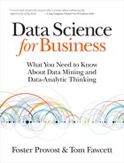
In addition to imposing upper and lower limits on term frequency, many systems take into account the distribution of the term over a corpus as well. The fewer documents in which a term occurs, the more significant it likely is to be to the documents is does occur in. This sparseness of a term t is measured commonly by an equation called inverse document frequency (IDF), which is shown in Equation 10-1.

IDF may be thought of as the boost a term gets for being rare. Figure 10-1 shows a graph of IDF(t) as a function of the number of documents in which t occurs, in a corpus of 100 documents. As you can see, when a term is very rare (far left) the IDF is quite high. It decreases quickly as t becomes more common in documents, and asymptotes at 1.0. Most stopwords, due to their prevalence, will have an IDF near one.
Combining Them: TFIDF
A very popular representation for text is the product of Term Frequency (TF) and Inverse Document Frequency (IDF), commonly referred to as TFIDF. The TFIDF value of a term t in a given document d is thus:

Note that the TFIDF value is specific to a single document (d) whereas IDF depends on the entire corpus. Systems employing the bag-of-words representation typically go through steps of stemming and stopword elimination before doing term counts. Term counts within the documents form the TF values for each term, and the document counts across the corpus form the IDF values.
Each document thus becomes a feature vector, and the corpus is the set of these feature vectors. This set can then be used in a data mining algorithm for classification, clustering, or retrieval.
Because there are very many potential terms with text representation, feature selection is often employed. Systems do this in various ways, such as imposing minimum and maximum thresholds of term counts, and/or using a measure such as information gain[61] to rank the terms by importance so that low-gain terms can be culled.
The bag-of-words text representation approach treats every word in a document as an independent potential keyword (feature) of the document, then assigns values to each document based on frequency and rarity. TFIDF is a very common value representation for terms, but it is not necessarily optimal. If someone describes mining a text corpus using bag of words it just means they’re treating each word individually as a feature. Their values could be binary, term frequency, or TFIDF, with normalization or without. Data scientists develop intuitions about how best to attack a given text problem, but they’ll typically experiment with different representations to see which produces the best results.
Example: Jazz Musicians
Having introduced a few basic concepts, let’s now illustrate them with a concrete example: representing jazz musicians. Specifically, we’re going to look at a small corpus of 15 prominent jazz musicians and excerpts of their biographies from Wikipedia. Here are excerpts from a few jazz musician biographies:
- Charlie Parker
- Charles “Charlie” Parker, Jr., was an American jazz saxophonist and composer. Miles Davis once said, “You can tell the history of jazz in four words: Louis Armstrong. Charlie Parker.” Parker acquired the nickname “Yardbird” early in his career and the shortened form, “Bird,” which continued to be used for the rest of his life, inspired the titles of a number of Parker compositions, […]
- Duke Ellington
- Edward Kennedy “Duke” Ellington was an American composer, pianist, and big-band leader. Ellington wrote over 1,000 compositions. In the opinion of Bob Blumenthal of The Boston Globe, “in the century since his birth, there has been no greater composer, American or otherwise, than Edward Kennedy Ellington.” A major figure in the history of jazz, Ellington’s music stretched into various other genres, including blues, gospel, film scores, popular, and classical.[…]
- Miles Davis
- Miles Dewey Davis III was an American jazz musician, trumpeter, bandleader, and composer. Widely considered one of the most influential musicians of the 20th century, Miles Davis was, with his musical groups, at the forefront of several major developments in jazz music, including bebop, cool jazz, hard bop, modal jazz, and jazz fusion.[…]
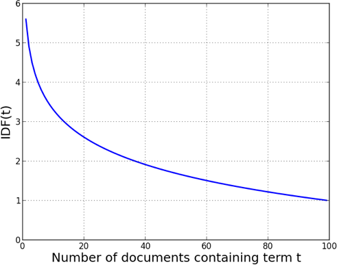
Even with this fairly small corpus of fifteen documents, the corpus and its vocabulary are too large to show here (nearly 2,000 features after stemming and stopword removal) so we can only illustrate with a sample. Consider the sample phrase “Famous jazz saxophonist born in Kansas who played bebop and latin.” We could imagine it being typed as a query to a search engine. How would it be represented? It is treated and processed just like a document, and goes through many of the same steps.
First, basic stemming is applied. Stemming methods are not perfect, and can produce
terms like kansa and famou from “Kansas” and “famous.” Stemming
perfection usually isn’t important as long as it’s consistent among all the documents.
The result is shown in Figure 10-2.
Next, stopwords (in and and) are removed, and the words are normalized with respect to document length. The result is shown in Figure 10-3.
These values would typically be used as the Term Frequency (TF) feature values if we were to stop here. Instead, we’ll generate the full TFIDF representation by multiplying each term’s TF value by its IDF value. As we said, this boosts words that are rare.
Jazz and play are very frequent in this corpus of jazz musician biographies so they get no boost from IDF. They are almost stopwords in this corpus.
The terms with the highest TFIDF values (“latin,” “famous,” and “kansas”) are the rarest in this corpus so they end up with the highest weights among the terms in the query. Finally, the terms are renormalized, producing the final TFIDF weights shown in Figure 10-4. This is the feature vector representation of this sample “document” (the query).

Having shown how this small “document” would be represented, let’s use it for something. Recall in Chapter 6, we discussed doing nearest-neighbor retrievals by employing a distance metric, and we showed how similar whiskies could be retrieved. We can do the same thing here. Assume our sample phrase “Famous jazz saxophonist born in Kansas who played bebop and latin” was a search query typed by a user and we were implementing a simple search engine. How might it work? First, we would translate the query to its TFIDF representation, as shown graphically in Figure 10-4. We’ve already computed TFIDF representations of each of our jazz musician biography documents. Now all we need to do is to compute the similarity of our query term to each musician’s biography and choose the closest one!
For doing this matching, we’ll use the Cosine Similarity function (Equation 6-5) discussed back in the starred section * Other Distance Functions. Cosine similarity is commonly used in text classification to measure the distance between documents.

| Musician | Similarity | Musician | Similarity | |
Charlie Parker | 0.135 | Count Basie | 0.119 | |
Dizzy Gillespie | 0.086 | John Coltrane | 0.079 | |
Art Tatum | 0.050 | Miles Davis | 0.050 | |
Clark Terry | 0.047 | Sun Ra | 0.030 | |
Dave Brubeck | 0.027 | Nina Simone | 0.026 | |
Thelonius Monk | 0.025 | Fats Waller | 0.020 | |
Charles Mingus | 0.019 | Duke Ellington | 0.017 | |
Benny Goodman | 0.016 | Louis Armstrong | 0.012 |
As you can see, the closest matching document is Charlie Parker—who was, in fact, a saxophonist born in Kansas and who played the bebop style of jazz. He sometimes combined other genres, including Latin, a fact that is mentioned in his biography.
* The Relationship of IDF to Entropy
Technical Details Ahead
Back in Selecting Informative Attributes, we introduced the entropy measure when we began discussing predictive modeling. The curious reader (with a long memory) may notice that Inverse Document Frequency and entropy are somewhat similar—they both seem to measure how “mixed” a set is with respect to a property. Is there any connection between the two? Maybe they’re the same? They are not identical, but they are related, and this section will show the relationship. If you’re not curious about this you can skip this section.
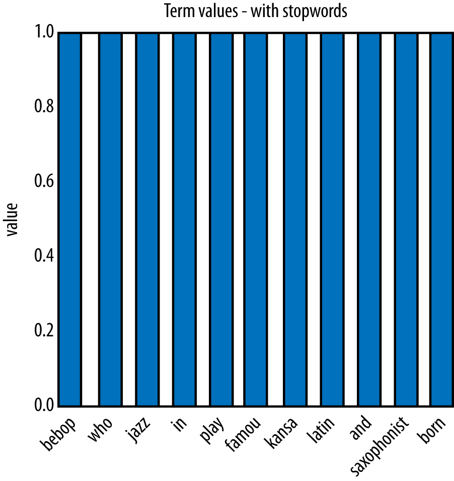
Figure 10-5 shows some graphs related to the equations we’re going to talk about. To begin, consider a term t in a document set. What is the probability that a term t occurs in a document set? We can estimate it as:
To simplify things, from here on we’ll refer to this estimate ![]() simply as p. Recall that the definition of IDF of some term t is:
simply as p. Recall that the definition of IDF of some term t is:

The 1 is just a constant so let’s discard it. We then notice that IDF(t) is basically log(1/p). You may recall from algebra that log(1/p) is equal to -log(p).
Consider again the document set with respect to a term t. Each document either contains t (with probability p) or does not contain it (with probability 1-p). Let’s create a pseudo, mirror-image term not_t that, by definition, occurs in every document that does not contain t. What’s the IDF of this new term? It is:

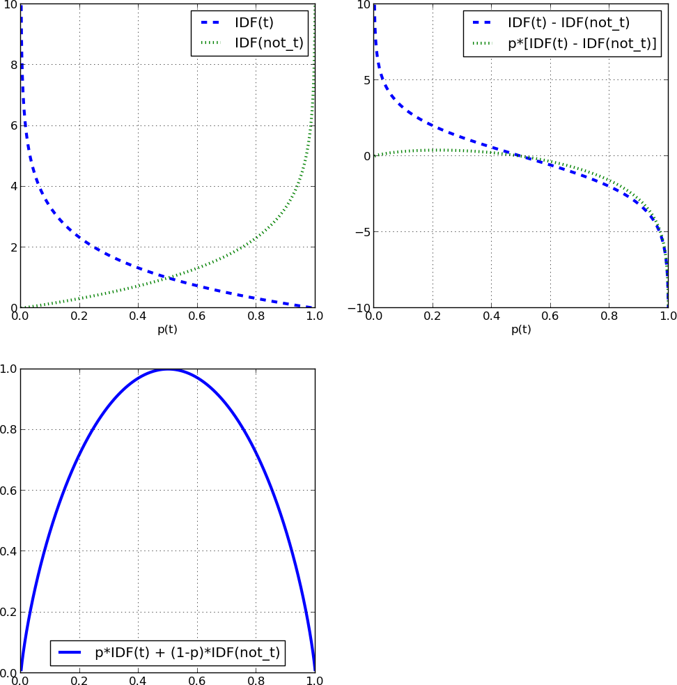
See the upper left graph of Figure 10-5. The two graphs are mirror images of each other, as we might expect. Now recall the definition of entropy from Equation 3-1. For a binary term where p2=1-p1, the entropy becomes:

In our case, we have a binary term t that either occurs (with probability p) or does not (with probability 1-p). So the definition of entropy of a set partitioned by t reduces to:

Now, given our definitions of IDF(t) and IDF(not_t), we can start substituting and simplifying (for reference, various of these subexpressions are plotted in the top right graph of Figure 10-5).
Note that this is now in the form of an expected value calculation! We can express entropy as the expected value of IDF(t) and IDF(not_t) based on the probability of the term’s occurrence in the corpus. Its graph at the bottom left in Figure 10-5 does match the entropy curve of Figure 3-3 back in Chapter 3.
Beyond Bag of Words
The basic bag of words approach is relatively simple and has much to recommend it. It requires no sophisticated parsing ability or other linguistic analysis. It performs surprisingly well on a variety of tasks, and is usually the first choice of data scientists for a new text mining problem.
Still, there are applications for which bag of words representation isn’t good enough and more sophisticated techniques must be brought to bear. Here we briefly discuss a few of them.
N-gram Sequences
As presented, the bag-of-words representation treats every individual word as
a term, discarding word order entirely. In some cases, word order is
important and you want to preserve some information about it in the
representation. A next step up in complexity is to include sequences of
adjacent words as terms. For example, we could include pairs of adjacent
words so that if a document contained the sentence “The quick brown fox
jumps.” it would be transformed into the set of its constituent words {quick, brown, fox, jumps},
plus the tokens quick_brown, brown_fox, and fox_jumps.
This general representation tactic is called n-grams. Adjacent pairs are commonly called bi-grams. If you hear a data scientist mention representing text as “bag of n-grams up to three” it simply means she’s representing each document using as features its individual words, adjacent word pairs, and adjacent word triples.
N-grams are useful when particular phrases are significant but their component
words may not be. In a business news story, the appearance of the tri-gram
exceed_analyst_expectation is more meaningful than simply knowing that the
individual words analyst, expectation, and exceed appeared somewhere in
a story. An advantage of using n-grams is that they are easy to generate;
they require no linguistic knowledge or complex parsing algorithm.
The main disadvantage of n-grams is that they greatly increase the size of the feature set. There are many adjacent word pairs, and still more adjacent word triples. The number of features generated can quickly get out of hand, and many of them will be very rare, occurring only once in the corpus. Data mining using n-grams almost always needs some special consideration for dealing with massive numbers of features, such as a feature selection stage or special consideration to computational storage space.
Named Entity Extraction
Sometimes we want still more sophistication in phrase extraction. We want to be able to recognize common named entities in documents. Silicon Valley, New York Mets, Department of the Interior, and Game of Thrones are significant phrases. Their component words mean one thing, and may not be significant, but in sequence they name unique entities with interesting identities. The basic bag-of-words (or even n-grams) representation may not capture these, and we’d want a preprocessing component that knows when word sequences constitute proper names.
Many text-processing toolkits include a named entity extractor of some sort.
Usually these can process raw text and extract phrases annotated with terms
like person or organization. In some cases normalization is done so that,
for example, phrases like “HP,” “H-P,” and “Hewlett-Packard” all link to
some common representation of the Hewlett-Packard Corporation.
Unlike bag of words and n-grams, which are based on segmenting text on whitespace and punctuation, named entity extractors are knowledge intensive. To work well, they have to be trained on a large corpus, or hand coded with extensive knowledge of such names. There is no linguistic principle dictating that the phrase “oakland raiders” should refer to the Oakland Raiders professional football team, rather than, say, a group of aggressive California investors. This knowledge has to be learned, or coded by hand. The quality of entity recognition can vary, and some extractors may have particular areas of expertise, such as industry, government, or popular culture.
Topic Models
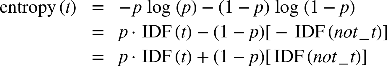
So far we’ve dealt with models created directly from words (or named entities) appearing from a document. The resulting model—whatever it may be—refers directly to words. Learning such direct models is relatively efficient, but is not always optimal. Because of the complexity of language and documents, sometimes we want an additional layer between the document and the model. In the context of text we call this the topic layer (see Figure 10-6).
The main idea of a topic layer is first to model the set of topics in a corpus separately. As before, each document constitutes a sequence of words, but instead of the words being used directly by the final classifier, the words map to one or more topics. The topics also are learned from the data (often via unsupervised data mining). The final classifier is defined in terms of these intermediate topics rather than words. One advantage is that in a search engine, for example, a query can use terms that do not exactly match the specific words of a document; if they map to the correct topic(s), the document will still be considered relevant to the search.
General methods for creating topic models include matrix factorization methods, such as Latent Semantic Indexing and Probabilistic Topic Models, such as Latent Dirichlet Allocation. The math of these approaches is beyond the scope of this book, but we can think of the topic layer as being a clustering of words. In topic modeling, the terms associated with the topic, and any term weights, are learned by the topic modeling process. As with clusters, the topics emerge from statistical regularities in the data. As such, they are not necessarily intelligible, and they are not guaranteed to correspond to topics familiar to people, though in many cases they are.
Note: Topics as Latent Information
Topic models are a type of latent information model, which we’ll discuss a bit more in Chapter 12 (along with a movie recommendation example). You can think of latent information as a type of intermediate, unobserved layer of information inserted between the inputs and outputs. The techniques are essentially the same for finding latent topics in text and for finding latent “taste” dimensions of movie viewers. In the case of text, words map to topics (unobserved) and topics map to documents. This makes the entire model more complex and more expensive to learn, but can yield better performance. In addition, the latent information is often interesting and useful in its own right (as we will see again in the movie recommendation example in Chapter 12).
Example: Mining News Stories to Predict Stock Price Movement
To illustrate some issues in text mining, we introduce a new predictive mining task: we’re going to predict stock price fluctuations based on the text of news stories. Roughly speaking, we are going to “predict the stock market” based on the stories that appear on the news wires. This project contains many common elements of text processing and of problem formulation.
The Task
Every trading day there is activity in the stock market. Companies make and announce decisions—mergers, new products, earnings projections, and so forth—and the financial news industry reports on them. Investors read these news stories, possibly change their beliefs about the prospects of the companies involved, and trade stock accordingly. This results in stock price changes. For example, announcements of acquisitions, earnings, regulatory changes, and so on can all affect the price of a stock, either because it directly affects the earnings potential or because it affects what traders think other traders are likely to pay for the stock.
This is a very simplified view of the financial markets, of course, but it’s enough to lay out a basic task. We want to predict stock price changes based on financial news. There are many ways we could approach this based on the ultimate purpose of the project. If we wanted to make trades based on financial news, ideally we’d like to predict—in advance and with precision—the change in a company’s stock price based on the stream of news. In reality there are many complex factors involved in stock price changes, many of which are not conveyed in news stories.
Instead, we’ll mine the news stories for a more modest purpose, that of news recommendation. From this point of view, there is a huge stream of market news coming in—some interesting, most not. We’d like predictive text mining to recommend interesting news stories that we should pay attention to. What’s an interesting story? Here we’ll define it as news that will likely result in a significant change in a stock’s price.
We have to simplify the problem further to make it more tractable (in fact, this task is a good example of problem formulation as much as it is of text mining). Here are some of the problems and simplifying assumptions:
- It is difficult to predict the effect of news far in advance. With many stocks, news arrives fairly often and the market responds quickly. It is unrealistic, for example, to predict what price a stock will have a week from now based on a news release today. Therefore, we’ll try to predict what effect a news story will have on stock price the same day.
- It is difficult to predict exactly what the stock price will be. Instead, we will be satisfied with the direction of movement: up, down, or no change. In fact, we’ll simplify this further into change and no change. This works well for our example application: recommending a news story if it looks like it will trigger, or indicate, a subsequent change in the stock price.
- It is difficult to predict small changes in stock price, so instead we’ll predict relatively large changes. This will make the signal a bit cleaner at the expense of yielding fewer events. We will deliberately ignore the subtlety of small fluctuations.
It is difficult to associate a specific piece of news with a price change. In principle, any piece of news could affect any stock. If we accepted this idea it would leave us with a huge problem of credit assignment: how do you decide which of today’s thousands of stories are relevant? We need to narrow the “causal radius.”
We will assume that only news stories mentioning a specific stock will affect that stock’s price. This is inaccurate, of course—companies are affected by the actions of their competitors, customers, and clients, and it’s rare that a news story will mention all of them. But for a first pass this is an acceptable simplifying assumption.
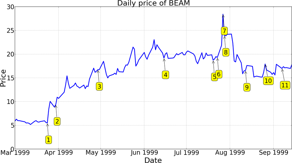
We still have to nail some of this down. Consider issue two. What is a “relatively large” change? We can (somewhat arbitrarily) place a threshold of 5%. If a stock’s price increases by five percent or more, we’ll call it a surge; if it declines by five percent or more, we’ll call it a plunge. What if it changes by some amount in between? We could call any value in between stable, but that’s cutting it a little close—a 4.9% change and a 5% change shouldn’t really be distinct classes. Instead, we’ll designate some “gray zones” to make the classes more separable (see Figure 10-7). Only if a stock’s price stays between 2.5% and −2.5% will it be called stable. Otherwise, for the zones between 2.5% to 5% and −2.5% to −5%, we’ll refuse to label it.

For the purpose of this example, we’ll create a two-class problem by merging surge and plunge into a single class, change. It will be the positive class, and stable (no change) will be the negative class.
The Data
The data we’ll use comprise two separate time series: the stream of news stories (text documents), and a corresponding stream of daily stock prices. The Internet has many sources of financial data, such as Google Finance and Yahoo! Finance. For example, to see what news stories are available about Apple Computer, Inc., see the corresponding Yahoo! Finance page. Yahoo! aggregates news stories from a variety of sources such as Reuters, PR Web, and Forbes. Historical stock prices can be acquired from many sources, such as Google Finance.
The data to be mined are historical data from 1999 for stocks listed on the New York Stock Exchange and NASDAQ. This data was used in a prior study (Fawcett & Provost, 1999). We have open and close prices for stocks on the major exchanges, and a large compendium of financial news stories throughout the year—nearly 36,000 stories altogether. Here is a sample news story from the corpus:
      1999-03-30 14:45:00
      WALTHAM, Mass.--(BUSINESS WIRE)--March 30, 1999--Summit Technology,
      Inc. (NASDAQ:BEAM) and Autonomous Technologies Corporation
      (NASDAQ:ATCI) announced today that the Joint Proxy/Prospectus for
      Summit's acquisition of Autonomous has been declared effective by the
      Securities and Exchange Commission. Copies of the document have been
      mailed to stockholders of both companies. "We are pleased that these
      proxy materials have been declared effective and look forward to the
      shareholder meetings scheduled for April 29," said Robert Palmisano,
      Summit's Chief Executive Officer.
As with many text sources, there is a lot of miscellaneous material since it is intended for human readers and not machine parsing (see Sidebar: The News Is Messy for more details). The story includes the date and time, the news source (Reuters), stock symbols and link (NASDAQ:BEAM), as well as background material not strictly germane to the news. Each such story is tagged with the stock mentioned.
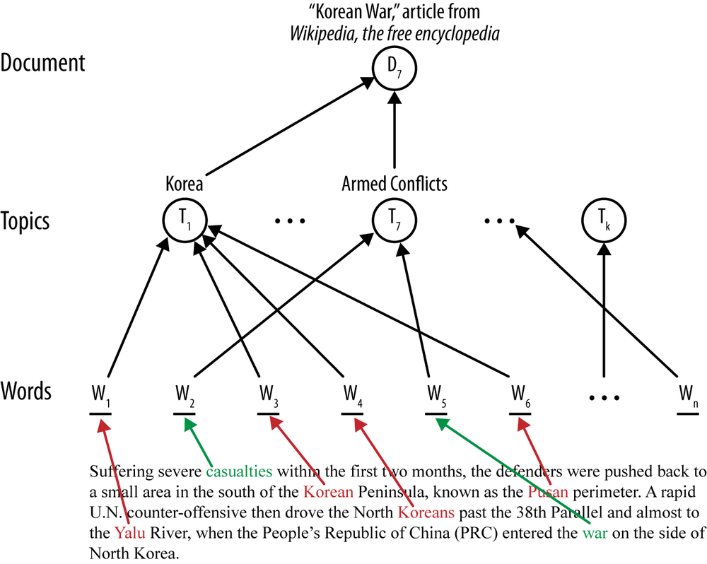
1 | Summit Tech announces revenues for the three months ended Dec 31, 1998 were $22.4 million, an increase of 13%. |
2 | Summit Tech and Autonomous Technologies Corporation announce that the Joint Proxy/Prospectus for Summit’s acquisition of Autonomous has been declared effective by the SEC. |
3 | Summit Tech said that its procedure volume reached new levels in the first quarter and that it had concluded its acquisition of Autonomous Technologies Corporation. |
4 | Announcement of annual shareholders meeting. |
5 | Summit Tech announces it has filed a registration statement with the SEC to sell 4,000,000 shares of its common stock. |
6 | A US FDA panel backs the use of a Summit Tech laser in LASIK procedures to correct nearsightedness with or without astigmatism. |
7 | Summit up 1-1/8 at 27-3/8. |
8 | Summit Tech said today that its revenues for the three months ended June 30, 1999 increased 14%… |
9 | Summit Tech announces the public offering of 3,500,000 shares of its common stock priced at $16/share. |
10 | Summit announces an agreement with Sterling Vision, Inc. for the purchase of up to six of Summit’s state of the art, Apex Plus Laser Systems. |
11 | Preferred Capital Markets, Inc. initiates coverage of Summit Technology Inc. with a Strong Buy rating and a 12-16 month price target of $22.50. |
Figure 10-8 shows the kind of data we have to work with. They are basically two linked time series. At the top is a graph of the stock price of Summit Technologies, Inc., a manufacturer of excimer laser systems for use in laser vision correction. Some points on the graph are annotated with story numbers on the date the story was released. Below the graph are summaries of each story.
Data Preprocessing
As mentioned, we have two streams of data. Each stock has an opening and closing price for the day, measured at 9:30 am EST and 4:00 pm EST, respectively. From these values we can easily compute a percentage change. There is one minor complication. We’re trying to predict stories that produce a substantial change in a stock’s value. Many events occur outside of trading hours, and fluctuations near the opening of trading can be erratic. For this reason, instead of measuring the opening price at the opening bell (9:30 am EST) we measure it at 10:00 am, and track the difference between the day’s prices at 4 pm and 10 am. Divided by the stock’s closing price, this becomes the daily percent change.
The stories require much more care. The stories are pre-tagged with stocks, which are mostly accurate (Sidebar: The News Is Messy goes into some details on why this is a difficult text mining problem). Almost all stories have timestamps (those without are discarded) so we can align them with the correct day and trading window. Because we want a fairly tight association of a story with the stock(s) it might affect, we reject any stories mentioning more than two stocks. This gets rid of many stories that are just summaries and news aggregations.
The basic steps outlined in Bag of Words were applied to reduce each story to a TFIDF representation. In particular, each word was case-normalized and stemmed, and stopwords were removed. Finally, we created n-grams up to two, such that every individual term and pair of adjacent terms were used to represent each story.
Subject to this preparation, each story is tagged with a label (change or no change) based on the associated stock(s) price movement, as depicted in Figure 10-7. This results in about 16,000 usable tagged stories. For reference, the breakdown of stories was about 75% no change, 13% surge, and 12% plunge. The surge and plunge stories were merged to form change, so 25% of the stories were followed by a significant price change to the stocks involved, and 75% were not.
Results
Before we dig into results, a short digression.
Previous chapters (particularly Chapter 7) stressed the importance of thinking carefully about the business problem being solved in order to frame the evaluation. With this example we have not done such careful specification. If the purpose of this task were to trigger stock trades, we might propose an overall trading strategy involving thresholds, time limits, and transaction costs, from which we could produce a complete cost-benefit analysis.[62] But the purpose is news recommendation (answering “which stories lead to substantial stock price changes?”) and we’ve left this pretty open, so we won’t specify exact costs and benefits of decisions. For this reason, expected value calculations and profit graphs aren’t really appropriate here.
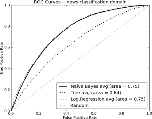
Instead, let’s look at predictability, just to get a sense of how well this problem can be solved. Figure 10-9 shows the ROC curves of three sample classifiers: Logistic Regression, Naive Bayes, and a Classification Tree, as well as the random classification line. These curves are averaged from ten-fold cross-validation, using change as the positive class and no change as the negative class. Several things are apparent. First, there is a significant “bowing out” of the curves away from the diagonal (Random) line, and the ROC curve areas (AUCs) are all substantially above 0.5, so there is predictive signal in the news stories. Second, logistic regression and Naive Bayes perform similarly, whereas the classification tree (Tree) is considerably worse. Finally, there is no obvious region of superiority (or deformity) in the curves. Bulges or concavities can sometimes reveal characteristics of the problem, or flaws in the data representation, but we see none here.
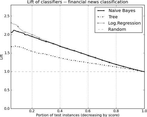
Figure 10-10 shows the corresponding lift curves of these three classifiers, again averaged from ten-fold cross-validation. Recall that one in four (25%) of the stories in our population is positive, (i.e., it is followed by a significant change in stock price). Each curve shows the lift in precision[63] we would get if we used the model to score and order the news stories. For example, consider the point at x=0.2, where the lifts of Logistic Regression and Naive Bayes are both around 2.0. This means that, if you were to score all the news stories and take the top 20% (x=0.2), you’d have twice the precision (lift of two) of finding a positive story in that group than in the population as a whole. Therefore, among the top 20% of the stories as ranked by the model, half are significant.
Before concluding this example, let’s look at some of the important terms found from this task. The goal of this example was not to create intelligible rules from the data, but prior work on the same corpus by Macskassy et al. (2001) did just that. Here is a list of terms with high information gain[64] taken from their work. Each term is either a word or a stem followed by suffixes in parentheses:
alert(s,ed), architecture, auction(s,ed,ing,eers), average(s,d), award(s,ed),
bond(s), brokerage, climb(ed,s,ing), close(d,s), comment(ator,ed,ing,s),
commerce(s), corporate, crack(s,ed,ing), cumulative, deal(s), dealing(s),
deflect(ed,ing), delays, depart(s,ed), department(s), design(ers,ing),
economy, econtent, edesign, eoperate, esource, event(s), exchange(s),
extens(ion,ive), facilit(y,ies), gain(ed,s,ing), higher, hit(s), imbalance(s),
index, issue(s,d), late(ly), law(s,ful), lead(s,ing), legal(ity,ly), lose,
majority, merg(ing,ed,es), move(s,d), online, outperform(s,ance,ed),
partner(s), payments, percent, pharmaceutical(s), price(d), primary,
recover(ed,s), redirect(ed,ion), stakeholder(s), stock(s), violat(ing,ion,ors)
Many of these are suggestive of significant announcements of good or bad news
for a company or its stock price. Some of them (econtent, edesign,
eoperate) are also suggestive of the “Dotcom Boom” of the late 1990s,
from which this corpus is taken, when the e- prefix was in vogue.
Though this example is one of the most complex presented in this book, it is still a fairly simple approach to mining financial news stories. There are many ways this project could be extended and refined. The bag-of-words representation is primitive for this task; named entity recognition could be used to better extract the names of the companies and people involved. Better still, event parsing should provide real leverage, since news stories usually report events rather than static facts about companies. It is not clear from individual words who are the subjects and objects of the events, and important modifiers like not, despite, and expect may not be adjacent to the phrases they modify, so the bag of words representation is at a disadvantage. Finally, to calculate price changes we considered only daily opening and closing stock prices, rather than hourly or instantaneous (“tick level”) price changes. The market responds quickly to news, and if we wanted to trade on the information we’d need to have fine-grained, reliable timestamps on both stock prices and news stories.
Summary
Our problems do not always present us with data in a neat feature vector representation that most data mining methods take as input. Real-world problems often require some form of data representation engineering to make them amenable to mining. Generally it is simpler to first try to engineer the data to match existing tools. Data in the form of text, images, sound, video, and spatial information usually require special preprocessing—and sometimes special knowledge on the part of the data science team.
In this chapter, we discussed one especially prevalent type of data that requires preprocessing: text. A common way to turn text into a feature vector is to break each document into individual words (its “bag of words” representation), and assign values to each term using the TFIDF formula. This approach is relatively simple, inexpensive and versatile, and requires little knowledge of the domain, at least initially. In spite of its simplicity, it performs surprisingly well on a variety of tasks. In fact, we will revisit these ideas on a completely different, nontext task in Chapter 14.
[59] Latin for “body.” The plural is corpora.
[60] Both of these examples appeared in recent search results on the film review site of a popular search engine. Not everyone is careful with stopword elimination.
[62] Some researchers have done this, evaluating their systems by simulating stock trades and calculating the return on investment. See, for example, Schumaker & Chen’s (2010) work on AZFinText.