Generally speaking, a model is a simplified representation of reality created to serve a purpose. It is simplified based on some assumptions about what is and is not important for the specific purpose, or sometimes based on constraints on information or tractability. For example, a map is a model of the physical world. It abstracts away a tremendous amount of information that the mapmaker deemed irrelevant for its purpose. It preserves, and sometimes further simplifies, the relevant information. For example, a road map keeps and highlights the roads, their basic topology, their relationships to places one would want to travel, and other relevant information. Various professions have well-known model types: an architectural blueprint, an engineering prototype, the Black-Scholes model of option pricing, and so on. Each of these abstracts away details that are not relevant to their main purpose and keeps those that are.

In data science, a predictive model is a formula for estimating the unknown value of interest: the target. The formula could be mathematical, or it could be a logical statement such as a rule. Often it is a hybrid of the two. Given our division of supervised data mining into classification and regression, we will consider classification models (and class-probability estimation models) and regression models.

This is in contrast to descriptive modeling, where the primary purpose of the model is not to estimate a value but instead to gain insight into the underlying phenomenon or process. A descriptive model of churn behavior would tell us what customers who churn typically look like.^[13] A descriptive model must be judged in part on its intelligibility, and a less accurate model may be preferred if it is easier to understand. A predictive model may be judged solely on its predictive performance, although we will discuss why intelligibility is nonetheless important. The difference between these model types is not as strict as this may imply; some of the same techniques can be used for both, and usually one model can serve both purposes (though sometimes poorly). Sometimes much of the value of a predictive model is in the understanding gained from looking at it rather than in the predictions it makes.

Before we discuss predictive modeling further, we must introduce some terminology. Supervised learning is model creation where the model describes a relationship between a set of selected variables (attributes or features) and a predefined variable called the target variable. The model estimates the value of the target variable as a function (possibly a probabilistic function) of the features. So, for our churn-prediction problem we would like to build a model of the propensity to churn as a function of customer account attributes, such as age, income, length with the company, number of calls to customer service, overage charges, customer demographics, data usage, and others.

Figure 3-1 illustrates some of the terminology we introduce here, in an oversimplified example problem of credit write-off prediction. An instance or example represents a fact or a data point—in this case a historical customer who had been given credit. This is also called a row in database or spreadsheet terminology. An instance is described by a set of attributes (fields, columns, variables, or features). An instance is also sometimes called a feature vector, because it can be represented as a fixed-length ordered collection (vector) of feature values. Unless stated otherwise, we will assume that the values of all the attributes (but not the target) are present in the data.

The creation of models from data is known as model induction. Induction is a term from philosophy that refers to generalizing from specific cases to general rules (or laws, or truths). Our models are general rules in a statistical sense (they usually do not hold 100% of the time; often not nearly), and the procedure that creates the model from the data is called the induction algorithm or learner. Most inductive procedures have variants that induce models both for classification and for regression. We will discuss mainly classification models because they tend to receive less attention in other treatments of statistics, and because they are relevant to many business problems (and thus much work in data science focuses on classification).

The input data for the induction algorithm, used for inducing the model, are called the training data. As mentioned in Chapter 2, they are called labeled data because the value for the target variable (the label) is known.

Let’s return to our example churn problem. Based on what we learned in Chapter 1 and Chapter 2, we might decide that in the modeling stage we should build a “supervised segmentation” model, which divides the sample into segments having (on average) higher or lower tendency to leave the company after contract expiration. To think about how this might be done, let’s now turn to one of our fundamental concepts: How can we select one or more attributes/features/variables that will best divide the sample with respect to our target variable of interest?

Recall that a predictive model focuses on estimating the value of some particular target variable of interest. An intuitive way of thinking about extracting patterns from data in a supervised manner is to try to segment the population into subgroups that have different values for the target variable (and within the subgroup the instances have similar values for the target variable). If the segmentation is done using values of variables that will be known when the target is not, then these segments can be used to predict the value of the target variable. Moreover, the segmentation may at the same time provide a human-understandable set of segmentation patterns. One such segment expressed in English might be: “Middle-aged professionals who reside in New York City on average have a churn rate of 5%.” Specifically, the term “middle-aged professionals who reside in New York City” is the definition of the segment (which references some particular attributes) and “a churn rate of 5%” describes the predicted value of the target variable for the segment.^[14]

Often we are interested in applying data mining when we have many attributes, and are not sure exactly what the segments should be. In our churn-prediction problem, who is to say what are the best segments for predicting the propensity to churn? If there exist in the data segments with significantly different (average) values for the target variable, we would like to be able to extract them automatically.

This brings us to our fundamental concept: how can we judge whether a variable contains important information about the target variable? How much? We would like automatically to get a selection of the more informative variables with respect to the particular task at hand (namely, predicting the value of the target variable). Even better, we might like to rank the variables by how good they are at predicting the value of the target.

Consider just the selection of the single most informative attribute. Solving this problem will introduce our first concrete data mining technique—simple, but easily extendable to be very useful. In our example, what variable gives us the most information about the future churn rate of the population? Being a professional? Age? Place of residence? Income? Number of complaints to customer service? Amount of overage charges?

We now will look carefully into one useful way to select informative variables, and then later will show how this technique can be used repeatedly to build a supervised segmentation. While very useful and illustrative, please keep in mind that direct, multivariate supervised segmentation is just one application of this fundamental idea of selecting informative variables. This notion should become one of your conceptual tools when thinking about data science problems more generally. For example, as we go forward we will delve into other modeling approaches, ones that do not incorporate variable selection directly. When the world presents you with very large sets of attributes, it may be (extremely) useful to harken back to this early idea and to select a subset of informative attributes. Doing so can substantially reduce the size of an unwieldy dataset, and as we will see, often will improve the accuracy of the resultant model.

Selecting Informative Attributes

Given a large set of examples, how do we select an attribute to partition them in an informative way? Let’s consider a binary (two class) classification problem, and think about what we would like to get out of it. To be concrete, Figure 3-2 shows a simple segmentation problem: twelve people represented as stick figures. There are two types of heads: square and circular; and two types of bodies: rectangular and oval; and two of the people have gray bodies while the rest are white.

Figure 3-2. A set of people to be classified. The label over each head represents the value of the target variable (write-off or not). Colors and shapes represent different predictor attributes.

These are the attributes we will use to describe the people. Above each person is the binary target label, Yes or No, indicating (for example) whether the person becomes a loan write-off. We could describe the data on these people as:

• Attributes:

  • head-shape: square, circular
  • body-shape: rectangular, oval
  • body-color: gray, white

• Target variable:

  • write-off: Yes, No

So let’s ask ourselves: which of the attributes would be best to segment these people into groups, in a way that will distinguish write-offs from non-write-offs? Technically, we would like the resulting groups to be as pure as possible. By pure we mean homogeneous with respect to the target variable. If every member of a group has the same value for the target, then the group is pure. If there is at least one member of the group that has a different value for the target variable than the rest of the group, then the group is impure.

Unfortunately, in real data we seldom expect to find a variable that will make the segments pure. However, if we can reduce the impurity substantially, then we can both learn something about the data (and the corresponding population), and importantly for this chapter, we can use the attribute in a predictive model—in our example, predicting that members of one segment will have higher or lower write-off rates than those in another segment. If we can do that, then we can for example offer credit to those with the lower predicted write-off rates, or can offer different credit terms based on the different predicted write-off rates.

Technically, there are several complications:

1. Attributes rarely split a group perfectly. Even if one subgroup happens to be pure, the other may not. For example, in Figure 3-2, consider if the second person were not there. Then body-color=gray would create a pure segment (write-off=no). However, the other associated segment, body-color=white, still is not pure.
2. In the prior example, the condition body-color=gray only splits off one single data point into the pure subset. Is this better than another split that does not produce any pure subset, but reduces the impurity more broadly?

3. Not all attributes are binary; many attributes have three or more distinct values. We must take into account that one attribute can split into two groups while another might split into three groups, or seven. How do we compare these?

4. Some attributes take on numeric values (continuous or integer). Does it make sense to make a segment for every numeric value? (No.) How should we think about creating supervised segmentations using numeric attributes?

Fortunately, for classification problems we can address all the issues by creating a formula that evaluates how well each attribute splits a set of examples into segments, with respect to a chosen target variable. Such a formula is based on a purity measure.

The most common splitting criterion is called information gain, and it is based on a purity measure called entropy. Both concepts were invented by one of the pioneers of information theory, Claude Shannon, in his seminal work in the field (Shannon, 1948).

Entropy is a measure of disorder that can be applied to a set, such as one of our individual segments. Consider that we have a set of properties of members of the set, and each member has one and only one of the properties. In supervised segmentation, the member properties will correspond to the values of the target variable. Disorder corresponds to how mixed (impure) the segment is with respect to these properties of interest. So, for example, a mixed up segment with lots of write-offs and lots of non-write-offs would have high entropy.

More technically, entropy is defined as:

Equation 3-1. Entropy

Each p_i is the probability (the relative percentage) of property i within the set, ranging from p_i = 1 when all members of the set have property i, and p_i = 0 when no members of the set have property i. The … simply indicates that there may be more than just two properties (and for the technically minded, the logarithm is generally taken as base 2).

Since the entropy equation might not lend itself to intuitive understanding, Figure 3-3 shows a plot of the entropy of a set containing 10 instances of two classes, + and –. We can see then that entropy measures the general disorder of the set, ranging from zero at minimum disorder (the set has members all with the same, single property) to one at maximal disorder (the properties are equally mixed). Since there are only two classes, p₊ = 1–p_–. Starting with all negative instances at the lower left, p₊ = 0, the set has minimal disorder (it is pure) and the entropy is zero. If we start to switch class labels of elements of the set from – to +, the entropy increases. Entropy is maximized at 1 when the instance classes are balanced (five of each), and p₊ = p_– = 0.5. As more class labels are switched, the + class starts to predominate and the entropy lowers again. When all instances are positive, p₊ = 1 and entropy is minimal again at zero.

Figure 3-3. Entropy of a two-class set as a function of p(+).

As a concrete example, consider a set S of 10 people with seven of the non-write-off class and three of the write-off class. So:

Entropy is only part of the story. We would like to measure how informative an attribute is with respect to our target: how much gain in information it gives us about the value of the target variable. An attribute segments a set of instances into several subsets. Entropy only tells us how impure one individual subset is. Fortunately, with entropy to measure how disordered any set is, we can define information gain (IG) to measure how much an attribute improves (decreases) entropy over the whole segmentation it creates. Strictly speaking, information gain measures the change in entropy due to any amount of new information being added; here, in the context of supervised segmentation, we consider the information gained by splitting the set on all values of a single attribute. Let’s say the attribute we split on has k different values. Let’s call the original set of examples the parent set, and the result of splitting on the attribute values the k children sets. Thus, information gain is a function of both a parent set and of the children resulting from some partitioning of the parent set—how much information has this attribute provided? That depends on how much purer the children are than the parent. Stated in the context of predictive modeling, if we were to know the value of this attribute, how much would it increase our knowledge of the value of the target variable?

Specifically, the definition of information gain (IG) is:

Equation 3-2. Information gain

Notably, the entropy for each child (c_i) is weighted by the proportion of instances belonging to that child, p(c_i). This addresses directly our concern from above that splitting off a single example, and noticing that that set is pure, may not be as good as splitting the parent set into two nice large, relatively pure subsets, even if neither is pure.

As an example, consider the split in Figure 3-4. This is a two-class problem (• and ★). Examining the figure, the children sets certainly seem “purer” than the parent set. The parent set has 30 instances consisting of 16 dots and 14 stars, so:

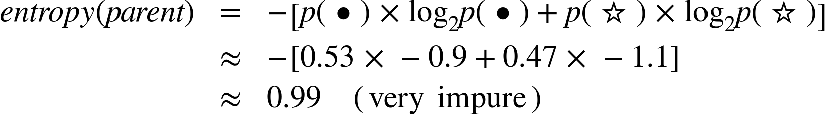
The entropy of the left child is:

The entropy of the right child is:

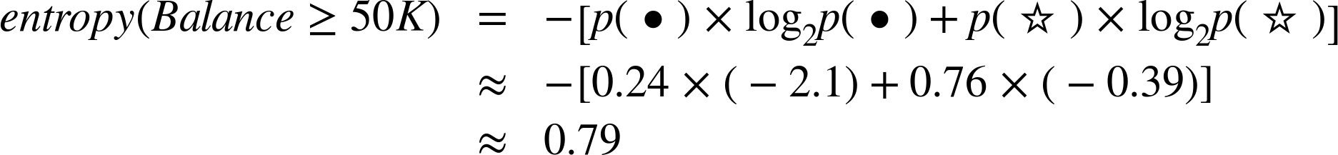
Using Equation 3-2, the information gain of this split is:

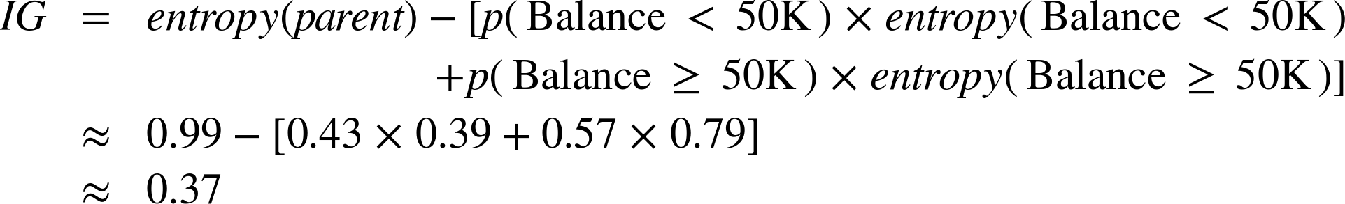
So this split reduces entropy substantially. In predictive modeling terms, the attribute provides a lot of information on the value of the target.

Figure 3-4. Splitting the “write-off” sample into two segments, based on splitting the Balance attribute (account balance) at 50K.

As a second example, consider another candidate split shown in Figure 3-5. This is the same parent set as in Figure 3-4, but instead we consider splitting on the attribute Residence with three values: OWN, RENT, and OTHER. Without showing the detailed calculations:

Figure 3-5. A classification tree split on the three-valued Residence attribute.

The Residence variable does have a positive information gain, but it is lower than that of Balance. Intuitively, this is because, while the one child Residence=OWN has considerably reduced entropy, the other values RENT and OTHER produce children that are no more pure than the parent. Thus, based on these data, the Residence variable is less informative than Balance.

Looking back at our concerns from above about creating supervised segmentation for classification problems, information gain addresses them all. It does not require absolute purity. It can be applied to any number of child subsets. It takes into account the relative sizes of the children, giving more weight to larger subsets.^[15]

Numeric variables

We have not discussed what exactly to do if the attribute is numeric. Numeric variables can be “discretized” by choosing a split point (or many split points) and then treating the result as a categorical attribute. For example, Income could be divided into two or more ranges. Information gain can be applied to evaluate the segmentation created by this discretization of the numeric attribute. We still are left with the question of how to choose the split point(s) for the numeric attribute. Conceptually, we can try all reasonable split points, and choose the one that gives the highest information gain.

Finally, what about supervised segmentations for regression problems—problems with a numeric target variable? Looking at reducing the impurity of the child subsets still makes intuitive sense, but information gain is not the right measure, because entropy-based information gain is based on the distribution of the properties in the segmentation. Instead, we would want a measure of the purity of the numeric (target) values in the subsets.

We will not go through a derivation here, but the fundamental idea is important: a natural measure of impurity for numeric values is variance. If the set has all the same values for the numeric target variable, then the set is pure and the variance is zero. If the numeric target values in the set are very different, then the set will have high variance. We can create a similar notion to information gain by looking at reductions in variance between parent and children. The process proceeds in direct analogy to the derivation for information gain above. To create the best segmentation given a numeric target, we might choose the one that produces the best weighted average variance reduction. In essence, we again would be finding variables that have the best correlation with the target, or alternatively, are most predictive of the target.

Example: Attribute Selection with Information Gain

Now we are ready to apply our first concrete data mining technique. For a dataset with instances described by attributes and a target variable, we can determine which attribute is the most informative with respect to estimating the value of the target variable. (We will delve into this more deeply below.) We also can rank a set of attributes by their informativeness, in particular by their information gain. This can be used simply to understand the data better. It can be used to help predict the target. Or it can be used to reduce the size of the data to be analyzed, by selecting a subset of attributes in cases where we can not or do not want to process the entire dataset.

To illustrate the use of information gain, we introduce a simple but realistic dataset taken from the machine learning dataset repository at the University of California at Irvine.^[16] It is a dataset describing edible and poisonous mushrooms taken from The Audubon Society Field Guide to North American Mushrooms. From the description:

This dataset includes descriptions of hypothetical samples corresponding to 23 species of gilled mushrooms in the Agaricus and Lepiota Family (pp. 500–525). Each species is identified as definitely edible, definitely poisonous, or of unknown edibility and not recommended. This latter class was combined with the poisonous one. The Guide clearly states that there is no simple rule for determining the edibility of a mushroom; no rule like “leaflets three, let it be” for Poisonous Oak and Ivy.

Each data example (instance) is one mushroom sample, described in terms of its observable attributes (the features). The twenty-odd attributes and the values for each are listed in Table 3-1. For a given example, each attribute takes on a single discrete value (e.g., gill-color=black). We use 5,644 examples from the dataset, comprising 2,156 poisonous and 3,488 edible mushrooms.

This is a classification problem because we have a target variable, called edible?, with two values yes (edible) and no (poisonous), specifying our two classes. Each of the rows in the training set has a value for this target variable. We will use information gain to answer the question: “Which single attribute is the most useful for distinguishing edible (edible?=Yes) mushrooms from poisonous (edible?=No) ones?” This is a basic attribute selection problem. In much larger problems we could imagine selecting the best ten or fifty attributes out of several hundred or thousand, and often you want do this if you suspect there are far too many attributes for your mining problem, or that many are not useful. Here, for simplicity, we will find the single best attribute instead of the top ten.

Table 3-1. The attributes of the Mushroom dataset

Attribute name	Possible values
CAP-SHAPE	bell, conical, convex, flat, knobbed, sunken
CAP-SURFACE	fibrous, grooves, scaly, smooth
CAP-COLOR	brown, buff, cinnamon, gray, green, pink, purple, red, white, yellow
BRUISES?	yes, no
ODOR	almond, anise, creosote, fishy, foul, musty, none,       pungent, spicy
GILL-ATTACHMENT	attached, descending, free, notched
GILL-SPACING	close, crowded, distant
GILL-SIZE	broad, narrow
GILL-COLOR	black, brown, buff, chocolate, gray, green, orange, pink, purple, red, white, yellow
STALK-SHAPE	enlarging, tapering
STALK-ROOT	bulbous, club, cup, equal, rhizomorphs, rooted, missing
STALK-SURFACE-ABOVE-RING	fibrous, scaly, silky, smooth
STALK-SURFACE-BELOW-RING	fibrous, scaly, silky, smooth
STALK-COLOR-ABOVE-RING	brown, buff, cinnamon, gray, orange, pink, red, white,     yellow
STALK-COLOR-BELOW-RING	brown, buff, cinnamon, gray, orange, pink, red, white,     yellow
VEIL-TYPE	partial, universal
VEIL-COLOR	brown, orange, white, yellow
RING-NUMBER	none, one, two
RING-TYPE	cobwebby, evanescent, flaring, large, none, pendant, sheathing, zone
SPORE-PRINT-COLOR	black, brown, buff, chocolate, green, orange, purple, white, yellow
POPULATION	abundant, clustered, numerous, scattered, several, solitary
HABITAT	grasses, leaves, meadows, paths, urban, waste, woods
EDIBLE? (Target variable)	yes, no

Since we now have a way to measure information gain this is straightforward: we are asking for the single attribute that gives the highest information gain.

To do this, we calculate the information gain achieved by splitting on each attribute. The information gain from Equation 3-2 is defined on a parent and a set of children. The parent in each case is the whole dataset. First we need entropy(parent), the entropy of the whole dataset. If the two classes were perfectly balanced in the dataset it would have an entropy of 1. This dataset is slightly unbalanced (more edible than poisonous mushrooms are represented) and its entropy is 0.96.

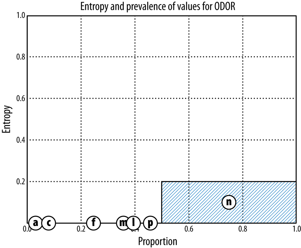
To illustrate entropy reduction graphically, we’ll show a number of entropy graphs for the mushroom domain (Figure 3-6 through Figure 3-8). Each graph is a two-dimensional description of the entire dataset’s entropy as it is divided in various ways by different attributes. On the x axis is the proportion of the dataset (0 to 1), and on the y axis is the entropy (also 0 to 1) of a given piece of the data. The amount of shaded area in each graph represents the amount of entropy in the dataset when it is divided by some chosen attribute (or not divided, in the case of Figure 3-6). Our goal of having the lowest entropy corresponds to having as little shaded area as possible.

The first chart, Figure 3-6, shows the entropy of the entire dataset. In such a chart, the highest possible entropy corresponds to the entire area being shaded; the lowest possible entropy corresponds to the entire area being white. Such a chart is useful for visualizing information gain from different partitions of a dataset, because any partition can be shown simply as slices of the graph (with widths corresponding to the proportion of the dataset), each with its own entropy. The weighted sum of entropies in the information gain calculation will be depicted simply by the total amount of shaded area.

Figure 3-6. Entropy chart for the entire Mushroom dataset. The entropy for the entire dataset is 0.96, so 96% of the area is shaded.

Figure 3-7. Entropy chart for the Mushroom dataset as split by GILL-COLOR. The amount of shading corresponds to the total (weighted sum) entropy, with each bar corresponding to the entropy of one of the attribute’s values, and the width of the bar corresponding to the prevalence of that value in the data.

For our entire dataset, the global entropy is 0.96, so Figure 3-6 shows a large shaded area below the line y = 0.96. We can think of this as our starting entropy—any informative attribute should produce a new graph with less shaded area. Now we show the entropy charts of three sample attributes. Each value of an attribute occurs in the dataset with a different frequency, so each attribute splits the set in a different way.

Figure 3-7 shows the dataset split apart by the attribute GILL-COLOR, whose values are coded as y (yellow), u (purple), n (brown), and so on. The width of each attribute represents what proportion of the dataset has that value, and the height is its entropy. We can see that GILL-COLOR reduces the entropy somewhat; the shaded area in Figure 3-7 is considerably less than the area in Figure 3-6.

Figure 3-8. Entropy chart for the Mushroom dataset as split by SPORE-PRINT-COLOR. The amount of shading corresponds to the total (weighted sum) entropy, with each bar corresponding to the entropy of one of the attribute’s values, and the width of the bar corresponding to the prevalence of that value in the data.

Similarly, Figure 3-8 shows how SPORE-PRINT-COLOR decreases uncertainty (entropy). A few of the values, such as h (chocolate), specify the target value perfectly and thus produce zero-entropy bars. But notice that they don’t account for very much of the population, only about 30%.

Figure 3-9 shows the graph produced by ODOR. Many of the values, such as a (almond), c (creosote), and m (musty) produce zero-entropy partitions; only n (no odor) has a considerable entropy (about 20%). In fact, ODOR has the highest information gain of any attribute in the Mushroom dataset. It can reduce the dataset’s total entropy to about 0.1, which gives it an information gain of 0.96 – 0.1 = 0.86. What is this saying? Many odors are completely characteristic of poisonous or edible mushrooms, so odor is a very informative attribute to check when considering mushroom edibility.^[17] If you’re going to build a model to determine the mushroom edibility using only a single feature, you should choose its odor. If you were going to build a more complex model you might start with the attribute ODOR before considering adding others. In fact, this is exactly the topic of the next section.

Figure 3-9. Entropy chart for the Mushroom dataset as split by ODOR. The amount of shading corresponds to the total (weighted sum) entropy, with each bar corresponding to the entropy of one of the attribute’s values, and the width of the bar corresponding to the prevalence of that value in the data.

Supervised Segmentation with Tree-Structured Models

We have now introduced one of the fundamental ideas of data mining: finding informative attributes from the data. Let’s continue on the topic of creating a supervised segmentation, because as important as it is, attribute selection alone does not seem to be sufficient. If we select the single variable that gives the most information gain, we create a very simple segmentation. If we select multiple attributes each giving some information gain, it’s not clear how to put them together. Recall from earlier that we would like to create segments that use multiple attributes, such as “Middle-aged professionals who reside in New York City on average have a churn rate of 5%.” We now introduce an elegant application of the ideas we’ve developed for selecting important attributes, to produce a multivariate (multiple attribute) supervised segmentation.

Consider a segmentation of the data to take the form of a “tree,” such as that shown in Figure 3-10. In the figure, the tree is upside down with the root at the top. The tree is made up of nodes, interior nodes and terminal nodes, and branches emanating from the interior nodes. Each interior node in the tree contains a test of an attribute, with each branch from the node representing a distinct value, or range of values, of the attribute. Following the branches from the root node down (in the direction of the arrows), each path eventually terminates at a terminal node, or leaf. The tree creates a segmentation of the data: every data point will correspond to one and only one path in the tree, and thereby to one and only one leaf. In other words, each leaf corresponds to a segment, and the attributes and values along the path give the characteristics of the segment. So the rightmost path in the tree in Figure 3-10 corresponds to the segment “Older, unemployed people with high balances.” The tree is a supervised segmentation, because each leaf contains a value for the target variable. Since we are talking about classification, here each leaf contains a classification for its segment. Such a tree is called a classification tree or more loosely a decision tree.

Classification trees often are used as predictive models—“tree structured models.” In use, when presented with an example for which we do not know its classification, we can predict its classification by finding the corresponding segment and using the class value at the leaf. Mechanically, one would start at the root node and descend through the interior nodes, choosing branches based on the specific attribute values in the example. The nonleaf nodes are often referred to as “decision nodes,” because when descending through the tree, at each node one uses the values of the attribute to make a decision about which branch to follow. Following these branches ultimately leads to a final decision about what class to predict: eventually a terminal node is reached, which gives a class prediction. In a tree, no two parents share descendants and there are no cycles; the branches always “point downwards” so that every example always ends up at a leaf node with some specific class determination.

Consider how we would use the classification tree in Figure 3-10 to classify an example of the person named Claudio from Figure 3-1. The values of Claudio’s attributes are Balance=115K, Employed=No, and Age=40. We begin at the root node that tests Employed. Since the value is No we take the right branch. The next test is Balance. The value of Balance is 115K, which is greater than 50K so we take a right branch again to a node that tests Age. The value is 40 so we take the left branch. This brings us to a leaf node specifying class=Not Write-off, representing a prediction that Claudio will not default. Another way of saying this is that we have classified Claudio into a segment defined by (Employed=No, Balance=115K, Age<45) whose classification is Not Write -off.

Figure 3-10. A simple classification tree.

Classification trees are one sort of tree-structured model. As we will see later, in business applications often we want to predict the probability of membership in the class (e.g., the probability of churn or the probability of write-off), rather than the class itself. In this case, the leaves of the probability estimation tree would contain these probabilities rather than a simple value. If the target variable is numeric, the leaves of the regression tree contain numeric values. However, the basic idea is the same for all.

Trees provide a model that can represent exactly the sort of supervised segmentation we often want, and we know how to use such a model to predict values for new cases (in “use”). However, we still have not addressed how to create such a model from the data. We turn to that now.

There are many techniques to induce a supervised segmentation from a dataset. One of the most popular is to create a tree-structured model (tree induction). These techniques are popular because tree models are easy to understand, and because the induction procedures are elegant (simple to describe) and easy to use. They are robust to many common data problems and are relatively efficient. Most data mining packages include some type of tree induction technique.

How do we create a classification tree from data? Combining the ideas introduced above, the goal of the tree is to provide a supervised segmentation—more specifically, to partition the instances, based on their attributes, into subgroups that have similar values for their target variables. We would like for each “leaf” segment to contain instances that tend to belong to the same class.

To illustrate the process of classification tree induction, consider the very simple example set shown previously in Figure 3-2.

Figure 3-11. First partitioning: splitting on body shape (rectangular versus oval).

Tree induction takes a divide-and-conquer approach, starting with the whole dataset and applying variable selection to try to create the “purest” subgroups possible using the attributes. In the example, one way is to separate people based on their body type: rectangular versus oval. This creates the two groups shown in Figure 3-11. How good is this partitioning? The rectangular-body people on the left are mostly Yes, with a single No person, so it is mostly pure. The oval-body group on the right has mostly No people, but two Yes people. This step is simply a direct application of the attribute selection ideas presented above. Let’s consider this “split” to be the one that yields the largest information gain.

Looking at Figure 3-11, we can now see the elegance of tree induction, and why it resonates well with so many people. The left and right subgroups are simply smaller versions of the problem with which we initially were faced! We can simply take each data subset and recursively apply attribute selection to find the best attribute to partition it. So in our example, we recursively consider the oval-body group (Figure 3-12). To split this group again we now consider another attribute: head shape. This splits the group in two on the right side of the figure. How good is this partitioning? Each new group has a single target label: four (square heads) of No, and two (round heads) of Yes. These groups are “maximally pure” with respect to class labels and there is no need to split them further.

Figure 3-12. Second partitioning: the oval body people sub-grouped by head type.

Figure 3-13. Third partitioning: the rectangular body people subgrouped by body color.

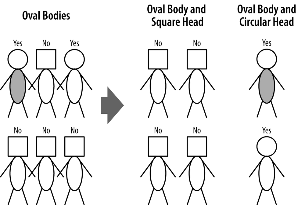
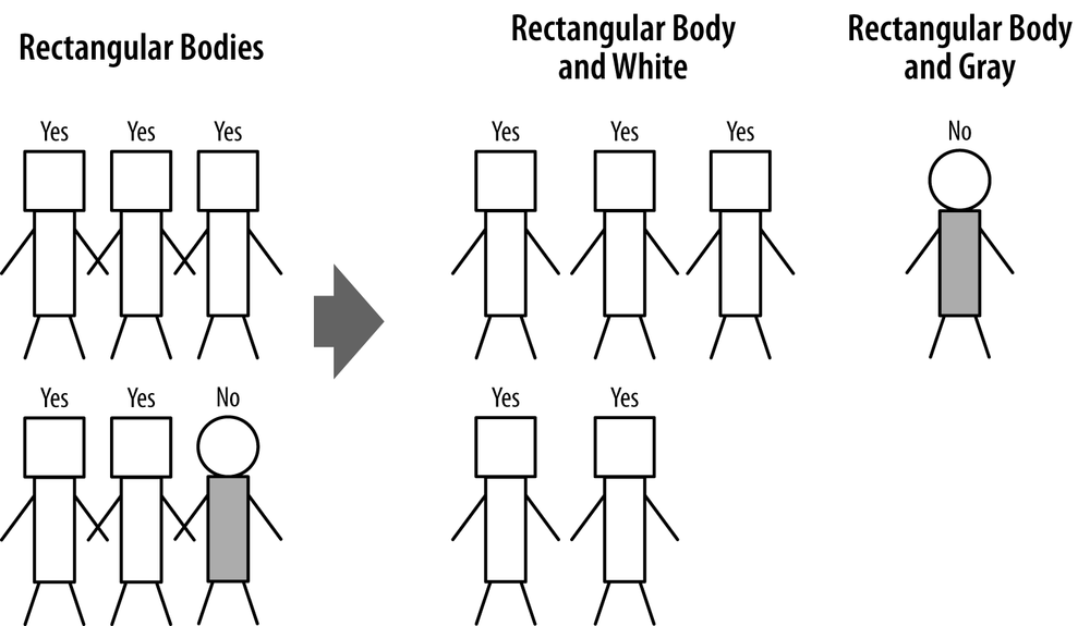
We still have not done anything with the rectangular body group on the left side of Figure 3-11, so let’s consider how to split them. There are five Yes people and one No person. There are two attributes we could split upon: head shape (square or round), and body color (white or gray). Either of these would work, so we arbitrarily choose body color. This produces the groupings in Figure 3-13. These are pure groups (all of one type) so we are finished. The classification tree corresponding to these groupings is shown in Figure 3-14.

Figure 3-14. The classification tree resulting from the splits done in Figure 3-11 to Figure 3-13.

In summary, the procedure of classification tree induction is a recursive process of divide and conquer, where the goal at each step is to select an attribute to partition the current group into subgroups that are as pure as possible with respect to the target variable. We perform this partitioning recursively, splitting further and further until we are done. We choose the attributes to split upon by testing all of them and selecting whichever yields the purest subgroups. When are we done? (In other words, when do we stop recursing?) It should be clear that we would stop when the nodes are pure, or when we run out of variables to split on. But we may want to stop earlier; we will return to this question in Chapter 5.

Continuing with the metaphor of predictive model building as supervised segmentation, it is instructive to visualize exactly how a classification tree partitions the instance space. The instance space is simply the space described by the data features. A common form of instance space visualization is a scatterplot on some pair of features, used to compare one variable against another to detect correlations and relationships.

Though data may contain dozens or hundreds of variables, it is only really possible to visualize segmentations in two or three dimensions at once. Still, visualizing models in instance space in a few dimensions is useful for understanding the different types of models because it provides insights that apply to higher dimensional spaces as well. It may be difficult to compare very different families of models just by examining their form (e.g., a mathematical formula versus a set of rules) or the algorithms that generate them. Often it is easier to compare them based on how they partition the instance space.

For example, Figure 3-15 shows a simple classification tree next to a two-dimensional graph of the instance space: Balance on the x axis and Age on the y axis. The root node of the classification tree tests Balance against a threshold of 50K. In the graph, this corresponds to a vertical line at 50K on the x axis splitting the plane into Balance<50K and Balance≥50K. At the left of this line lie the instances whose Balance values are less than 50K; there are 13 examples of class Write-off (black dot) and 2 examples of class non-Write-off (plus sign) in this region.

On the right branch out of the root node are instances with Balance≥50K. The next node in the classification tree tests the Age attribute against the threshold 45. In the graph this corresponds to the horizontal dotted line at Age=45. It appears only on the right side of the graph because this partition only applies to examples with Balance≥50. The Age decision node assigns to its left branch instances with Age<45, corresponding to the lower right segment of the graph, representing: (Balance≥50K AND Age<45).

Notice that each internal (decision) node corresponds to a split of the instance space. Each leaf node corresponds to an unsplit region of the space (a segment of the population). Whenever we follow a path in the tree out of a decision node we are restricting attention to one of the two (or more) subregions defined by the split. As we descend through a classification tree we consider progressively more focused subregions of the instance space.

Figure 3-15. A classification tree and the partitions it imposes in instance space. The black dots correspond to instances of the class Write-off, the plus signs correspond to instances of class non-Write-off. The shading shows how the tree leaves correspond to segments of the population in instance space.

Before moving on from the interpretation of classification trees, we should mention their interpretation as logical statements. Consider again the tree shown at the top of Figure 3-15. You classify a new unseen instance by starting at the root node and following the attribute tests downward until you reach a leaf node, which specifies the instance’s predicted class. If we trace down a single path from the root node to a leaf, collecting the conditions as we go, we generate a rule. Each rule consists of the attribute tests along the path connected with AND. Starting at the root node and choosing the left branches of the tree, we get the rule:

IF (Balance < 50K) AND (Age < 50) THEN Class=Write-off

We can do this for every possible path to a leaf node. From this tree we get three more rules:

IF (Balance < 50K) AND (Age ≥ 50) THEN Class=No Write-off
IF (Balance ≥ 50K) AND (Age < 45) THEN Class=Write-off
IF (Balance ≥ 50K) AND (Age ≥ 45) THEN Class=No Write-off

The classification tree is equivalent to this rule set. If these rules look repetitive, that’s because they are: the tree gathers common rule prefixes together toward the top of the tree. Every classification tree can be expressed as a set of rules this way. Whether the tree or the rule set is more intelligible is a matter of opinion; in this simple example, both are fairly easy to understand. As the model becomes larger, some people will prefer the tree or the rule set.

In many decision-making problems, we would like a more informative prediction than just a classification. For example, in our churn-prediction problem, rather than simply predicting whether a person will leave the company within 90 days of contract expiration, we would much rather have an estimate of the probability that he will leave the company within that time. Such estimates can be used for many purposes. We will discuss some of these in detail in later chapters, but briefly: you might then rank prospects by their probability of leaving, and then allocate a limited incentive budget to the highest probability instances. Alternatively, you may want to allocate your incentive budget to the instances with the highest expected loss, for which you’ll need (an estimate of) the probability of churn. Once you have such probability estimates you can use them in a more sophisticated decision-making process than these simple examples, as we’ll describe in later chapters.

There is another, even more insidious problem with models that give simple classifications, rather than estimates of class membership probability. Consider the problem of estimating credit default. Under normal circumstances, for just about any segment of the population to which we would be considering giving credit, the probability of write-off will be very small—far less than 0.5. In this case, when we build a model to estimate the classification (write-off or not), we’d have to say that for each segment, the members are likely not to default—and they will all get the same classification (not write-off). For example, in a naively built tree model every leaf will be labeled “not write-off.” This turns out to be a frustrating experience for new data miners: after all that work, the model really just says that no one is likely to default? This does not mean that the model is useless. It may be that the different segments indeed have very different probabilities of write-off, they just all are less than 0.5. If instead we use these probabilities for assigning credit, we may be able reduce our risk substantially.

So, in the context of supervised segmentation, we would like each segment (leaf of a tree model) to be assigned an estimate of the probability of membership in the different classes. Figure 3-15 more generally shows a “probability estimation tree” model for our simple write-off prediction example, giving not only a prediction of the class but also the estimate of the probability of membership in the class.^[18]

Fortunately, the tree induction ideas we have discussed so far can easily produce probability estimation trees instead of simple classification trees.^[19] Recall that the tree induction procedure subdivides the instance space into regions of class purity (low entropy). If we are satisfied to assign the same class probability to every member of the segment corresponding to a tree leaf, we can use instance counts at each leaf to compute a class probability estimate. For example, if a leaf contains n positive instances and m negative instances, the probability of any new instance being positive may be estimated as n/(n+m). This is called a frequency-based estimate of class membership probability.

At this point you may spot a problem with estimating class membership probabilities this way: we may be overly optimistic about the probability of class membership for segments with very small numbers of instances. At the extreme, if a leaf happens to have only a single instance, should we be willing to say that there is a 100% probability that members of that segment will have the class that this one instance happens to have?

This phenomenon is one example of a fundamental issue in data science (“overfitting”), to which we devote a chapter later in the book. For completeness, let’s quickly discuss one easy way to address this problem of small samples for tree-based class probability estimation. Instead of simply computing the frequency, we would often use a “smoothed” version of the frequency-based estimate, known as the Laplace correction, the purpose of which is to moderate the influence of leaves with only a few instances. The equation for binary class probability estimation becomes:

where n is the number of examples in the leaf belonging to class c, and m is the number of examples not belonging to class c.

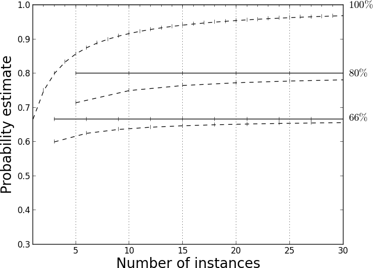
Let’s walk through an example with and without the Laplace correction. A leaf node with two positive instances and no negative instances would produce the same frequency-based estimate (p = 1) as a leaf node with 20 positive instances and no negatives. However, the first leaf node has much less evidence and may be extreme only due to there being so few instances. Its estimate should be tempered by this consideration. The Laplace equation smooths its estimate down to p = 0.75 to reflect this uncertainty; the Laplace correction has much less effect on the leaf with 20 instances (p ≈ 0.95). As the number of instances increases, the Laplace equation converges to the frequency-based estimate. Figure 3-16 shows the effect of Laplace correction on several class ratios as the number of instances increases (2/3, 4/5, and 1/1). For each ratio the solid horizontal line shows the uncorrected (constant) estimate, while the corresponding dashed line shows the estimate with the Laplace correction applied. The uncorrected line is the asymptote of the Laplace correction as the number of instances goes to infinity.

Now that we have a basic data mining technique for predictive modeling, let’s consider the churn problem again. How could we use tree induction to help solve it?

For this example, we have a historical data set of 20,000 customers. At the point of collecting the data, each customer either had stayed with the company or had left (churned). Each customer is described by the variables listed in Table 3-2.

Figure 3-16. The effect of Laplace smoothing on probability estimation for several instance ratios.

These variables comprise basic demographic and usage information available from the customer’s application and account. We want to use these data with our tree induction technique to predict which new customers are going to churn.

Before starting to build a classification tree with these variables, it is worth asking, How good are each of these variables individually? For this we measure the information gain of each attribute, as discussed earlier. Specifically, we apply Equation 3-2 to each variable independently over the entire set of instances, to see what each gains us.

The results are in Figure 3-17, with a table listing the exact values. As you can see, the first three variables—the house value, the number of leftover minutes, and the number of long calls per month—have a higher information gain than the rest.^[20] Perhaps surprisingly, neither the amount the phone is used nor the reported degree of satisfaction seems, in and of itself, to be very predictive of churning.

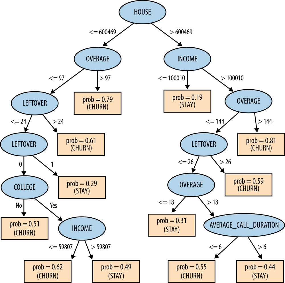
Applying a classification tree algorithm to the data, we get the tree shown in Figure 3-18. The highest information gain feature (HOUSE) according to Figure 3-17 is at the root of the tree. This is to be expected since it will always be chosen first. The second best feature, OVERAGE, also appears high in the tree. However, the order in which features are chosen for the tree doesn’t exactly correspond to their ranking in Figure 3-17. Why is this?

The answer is that the table ranks each feature by how good it is independently, evaluated separately on the entire population of instances. Nodes in a classification tree depend on the instances above them in the tree. Therefore, except for the root node, features in a classification tree are not evaluated on the entire set of instances. The information gain of a feature depends on the set of instances against which it is evaluated, so the ranking of features for some internal node may not be the same as the global ranking.

We have not yet discussed how we decide to stop building the tree. The dataset has 20,000 examples yet the tree clearly doesn’t have 20,000 leaf nodes. Can’t we just keep selecting more attributes to split upon, building the tree downwards until we’ve exhausted the data? The answer is yes, we can, but we should stop long before the model becomes that complex. This issue ties in closely with model generality and overfitting, whose discussion we defer to Chapter 5.

Figure 3-17. Churn attributes from Table 3-2 ranked by information gain.

Figure 3-18. Classification tree learned from the cellular phone churn data. Rectangular leaves correspond to segments of the population, defined by the path from the root at the top. Probabilities at the leaves are the estimated probabilities of churning for the corresponding segment; in parentheses are shown the classifications resulting from applying a decision threshold of 0.5 to the probabilities (i.e., are the individuals in the segment more likely to CHURN or to STAY?).

Consider a final issue with this dataset. After building a tree model from the data, we measured its accuracy against the data to see how good of a model it is. Specifically, we used a training set consisting half of people who churned and the other half who did not; after learning a classification tree from this, we applied the tree to the dataset to see how many of the examples it could classify correctly. The tree achieved 73% accuracy on its decisions. This raises two questions:

We will revisit these questions in Chapter 7 and Chapter 8, which delve into issues of model evaluation.

In this chapter, we introduced basic concepts of predictive modeling, one of the main tasks of data science, in which a model is built that can estimate the value of a target variable for a new unseen example. In the process, we introduced one of data science’s fundamental notions: finding and selecting informative attributes. Selecting informative attributes can be a useful data mining procedure in and of itself. Given a large collection of data, we now can find those variables that correlate with or give us information about another variable of interest. For example, if we gather historical data on which customers have or have not left the company (churned) shortly after their contracts expire, attribute selection can find demographic or account-oriented variables that provide information about the likelihood of customers churning. One basic measure of attribute information is called information gain, which is based on a purity measure called entropy; another is variance reduction.

Selecting informative attributes forms the basis of a common modeling technique called tree induction. Tree induction recursively finds informative attributes for subsets of the data. In so doing it segments the space of instances into similar regions. The partitioning is “supervised” in that it tries to find segments that give increasingly precise information about the quantity to be predicted, the target. The resulting tree-structured model partitions the space of all possible instances into a set of segments with different predicted values for the target. For example, when the target is a binary “class” variable such as churn versus not churn, or write-off versus not write-off, each leaf of the tree corresponds to a population segment with a different estimated probability of class membership.

Historically, tree induction has been a very popular data mining procedure because it is easy to understand, easy to implement, and computationally inexpensive. Research on tree induction goes back at least to the 1950s and 1960s. Some of the earliest popular tree induction systems include CHAID (Chi-squared Automatic Interaction Detection) (Kass, 1980) and CART (Classification and Regression Trees) (Breiman, Friedman, Olshen, & Stone, 1984), which are still widely used. C4.5 and C5.0 are also very popular tree induction algorithms, which have a notable lineage (Quinlan, 1986, 1993). J48 is a reimplementation of C4.5 in the Weka package (Witten & Frank, 2000; Hall et al., 2001).

In practice, tree-structured models work remarkably well, though they may not be the most accurate model one can produce from a particular data set. In many cases, especially early in the application of data mining, it is important that models be understood and explained easily. This can be useful not just for the data science team but for communicating results to stakeholders not knowledgeable about data mining.