Chapter 11. Decision Analytic Thinking II: Toward Analytical Engineering
Fundamental concept: Solving business problems with data science starts with analytical engineering: designing an analytical solution, based on the data, tools, and techniques available.
Exemplary technique: Expected value as a framework for data science solution design.
Ultimately, data science is about extracting information or knowledge from data, based on principled techniques. However, as we’ve discussed throughout the book, seldom does the world provide us with important business problems perfectly aligned with these techniques, or with data represented such that the techniques can be applied directly. Ironically, this fact often is better accepted by the business users (for whom it is often obvious) than by entry-level data scientists—because academic programs in statistics, machine learning, and data mining often present students with problems ready for the application of the tools that the programs teach.
Reality is much messier. Business problems rarely are classification problems or regression problems or clustering problems. They’re just business problems. Recall the mini-cycle in the first stages of the data mining process, where we focus on business understanding and data understanding. In these stages we must design or engineer a solution to the business problem. As with engineering more broadly, the data science team considers the needs of the business as well as the tools that might be brought to bear to solve the problem.
In this chapter, we will illustrate such analytical engineering with two case studies. In these case studies, we will see the application of the fundamental principles presented throughout the book, as well as some of the specific techniques that we have introduced. One common theme that runs through these case studies is how our expected value framework (recall from Chapter 7) helps to decompose each of the business problems into subproblems, such that the subproblems can be attacked with tried-and-true data science techniques. Then the expected value framework guides the recombination of the results into a solution to the original problem.
Targeting the Best Prospects for a Charity Mailing
A classic business problem for applying data science principles and techniques is targeted marketing. Targeted marketing makes for a perfect case study for two reasons. First, a very large number of businesses have problems that look similar to targeted marketing problems—traditional targeted (database) marketing, customer-specific coupon offers, online ad targeting, and so on. Second, the fundamental structure of the problem occurs in many other problems as well, such as our running example problem of churn management.
For this case study, let’s consider a real example of targeted marketing: targeting the best prospects for a charity mailing. Fundraising organizations (including those in universities) need to manage their budgets and the patience of their potential donors. In any given campaign segment, they would like to solicit from a “good” subset of the donors. This could be a very large subset for an inexpensive, infrequent campaign, or a smaller subset for a focused campaign that includes a not-so-inexpensive incentive package.
The Expected Value Framework: Decomposing the Business Problem and Recomposing the Solution Pieces
We would like to “engineer” an analytic solution to the problem, and our fundamental concepts will provide the structure to do so. To frame our data-analytic thinking, we begin by using the data-mining process (Chapter 2) to provide structure to the overall analysis: we start with business and data understanding. More specifically, we need to focus using one of our fundamental principles: what exactly is the business problem that we would like to solve (Chapter 7)?
So let’s get specific. A data miner might immediately think: we want to model the probability that each prospective customer, a prospective donor in this case, will respond to the offer. However, thinking carefully about the business problem we realize that in this case, the response can vary—some people might donate $100 while others might donate $1. We need to take this into account.
Would we like to maximize the total amount of donations? (The amount could be either in this particular campaign or over the lifetime of the donor prospects; let’s assume the first for simplicity.) What if we did that by targeting a massive number of people, and these each give just $1, and our costs are about $1 per person? We would make almost no money. So let’s revise our thinking.
Focusing on the business problem that we want to solve may have given us our answer right away, because to a business-savvy person it may seem rather obvious: we would like to maximize our donation profit—meaning the net after taking into account the costs. However, while we have methods for estimating the probability of response (that’s a clear application of class probability estimation over a binary outcome), it is not clear that we have methods to estimate profit.
Again, our fundamental concepts allow us to structure our thinking and engineer a data-analytic solution. Applying another one of our fundamental notions, we can structure this data analysis using the framework of expected value. We can apply the concepts introduced in Chapter 7 to our problem formulation: we can use expected value as a framework for structuring our approach to engineering a solution to the problem. Recall our formulation of the expected benefit (or cost) of targeting consumer x:

where ![]() is the probability of response
given consumer x, vR is the value we get from a response, and vNR is
the value we get from no response. Since everyone either responds or does not,
our estimate of the probability of not responding is just
is the probability of response
given consumer x, vR is the value we get from a response, and vNR is
the value we get from no response. Since everyone either responds or does not,
our estimate of the probability of not responding is just ![]() . As we discussed in
Chapter 7, we can model the probabilities by mining
historical data using one of the many techniques discussed through the book.
. As we discussed in
Chapter 7, we can model the probabilities by mining
historical data using one of the many techniques discussed through the book.
However, the expected value framework helps us realize that this business problem is slightly different from problems we have considered up to this point. In this case, the value varies from consumer to consumer, and we do not know the value of the donation that any particular consumer will give until after she is targeted! Let’s modify our formulation to make this explicit:

where vR(x) is the value we get from a response from consumer x and vNR(x) is the value we get if consumer x does not respond. The value of a response, vR(x), would be the consumer’s donation minus the cost of the solicitation. The value of no response, vNR(x), in this application would be zero minus the cost of the solicitation. To be complete, we also want to estimate the benefit of not targeting, and then compare the two to make the decision of whether to target or not. The expected benefit of not targeting is simply zero—in this application, we do not expect consumers to donate spontaneously without a solicitation. That may not always be the case, but let’s assume it is here.
Why exactly does the expected value framework help us? Because we may be able to estimate vR(x) and/or vNR(x) from the data as well. Regression modeling estimates such values. Looking at historical data on consumers who have been targeted, we can use regression modeling to estimate how much a consumer will respond. Moreover, the expected value framework gives us even more precise direction: vR(x) is the value we would predict to get if a consumer were to respond — this would be estimated using a model trained only on consumers who have responded. This turns out to be a more useful prediction problem than the problem of estimating the response from a targeted consumer generally, because in this application the vast majority of consumers do not respond at all, and so the regression modeling would need somehow to differentiate between the cases where the value is zero because of non-response or the value is small because of the characteristics of the consumer.
Stepping back for a moment, this example illustrates why the expected value framework is so useful for decomposing business problems: as discussed in Chapter 7, the expected value is a summation of products of probabilities and values, and data science gives us methods to estimate both probabilities and values. To be clear, we may not need to estimate some of these quantities (like vNR(x), which we assume in this example is always zero), and estimating them well may be a nontrivial undertaking. The point is that the expected value framework provides a helpful decomposition of possibly complicated business problems into subproblems that we understand better how to solve. The framework also shows exactly how to put the pieces together. For our example problem (chosen for its straightforward derivation), the answer works out to the intuitively satisfying result: mail to those people whose estimated expected donation is greater than the cost associated with mailing! Mathematically, we simply look for those whose expected benefit of targeting is greater than zero, and simplify the inequality algebraically. Let dR(x) be the estimated donation if consumer x were to respond, and let c be the mailing cost. Then:

We always want this benefit to be greater than zero, so:
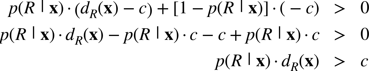
That is, the expected donation (lefthand side) should be greater than the solicitation cost (righthand side).
A Brief Digression on Selection Bias
This example brings up an important data science issue whose detailed treatment is beyond the scope of this book, but nevertheless is important to discuss briefly. For modeling the predicted donation, notice that the data may well be biased—meaning that they are not a random sample from the population of all donors. Why? Because the data are from past donations—from the individuals who did respond in the past. This is similar to the idea of modeling creditworthiness based on the experience with past credit customers: those are likely the people whom you had deemed to be creditworthy in the past! However, you want to apply the model to the general population to find good prospects. Why would those who happened to have been selected in the past be a good sample from which to model the general population? This is an example of selection bias—the data were not selected randomly from the population to which you intend to apply the model, but instead were biased in some way (by who happened to donate, and perhaps by those who were targeted using past methods; by who was granted credit in the past).
One important question for the data scientist is: do you expect the particular selection procedure that biases the data also to have a bearing on the value of the target variable? In modeling creditworthiness, the answer is absolutely yes—the past customers were selected precisely because they were predicted to be creditworthy. The donation case is not as straightforward, but it seems reasonable to expect that people who donate larger sums do not donate as often. For example, some people may donate $10 each and every time they’re asked. Others may give $100 and then feel they need not donate for a while, ignoring many subsequent campaigns. The result would be that those who happened to donate in some past campaign will be biased towards those who donate less.
Fortunately, there are data science techniques to help modelers deal with selection bias. They are beyond the scope of this book, but the interested reader might start by reading (Zadrozny & Elkan, 2001; Zadrozny, 2004) for an illustration of dealing with selection bias in this exact donation solicitation case study.
Our Churn Example Revisited with Even More Sophistication
Let’s return to our example of churn and apply what we’ve learned to examine it data-analytically. In our prior forays, we did not treat the problem as comprehensively as we might. That was by design, of course, because we had not learned everything we needed yet, and the intermediate attempts were illustrative. But now let’s examine the problem in more detail, applying the exact same fundamental data science concepts as we just applied to the case of soliciting donations.
The Expected Value Framework: Structuring a More Complicated Business Problem
First, what exactly is the business problem we would like to solve? Let’s keep our basic example problem setting: we’re having a serious problem with churn in our wireless business. Marketing has designed a special retention offer. Our task is to target the offer to some appropriate subset of our customer base.
Initially, we had decided that we would try to use our data to determine which customers would be the most likely to defect shortly after their contracts expire. Let’s continue to focus on the set of customers whose contracts are about to expire, because this is where most of the churn occurs. However, do we really want to target our offer to those with the highest probability of defection?
We need to go back to our fundamental concept: what exactly is the business problem we want to solve. Why is churn a problem? Because it causes us to lose money. The real business problem is losing money. If a customer actually were costly to us rather than profitable, we may not mind losing her. We would like to limit the amount of money we are losing—not simply to keep the most customers. Therefore, as in the donation problem, we want to take the value of the customer into account. Our expected value framework helps us to frame that analysis, similar to how it did above. In the case of churn, the value of an individual may be much easier to estimate: these are our customers, and since we have their billing records we can probably forecast their future value pretty well (contingent on their staying with the company) with a simple extrapolation of their past value. However, in this case we have not completely solved our problem, and framing the analysis using expected value shows why.
Let’s apply our expected value framework to really dig down into the business understanding/data understanding segment of the data mining process. Is there any problem with treating this case exactly as we did the donation case? As with the donation case study, we might represent the expected benefit of targeting a customer with the special offer as:

where ![]() is the probability that the
customer will Stay with the company after being targeted, vS(x) is
the value we get if consumer x stays with the company and vNS(x) is
the value we get if consumer x does not stay (defects or churns).
is the probability that the
customer will Stay with the company after being targeted, vS(x) is
the value we get if consumer x stays with the company and vNS(x) is
the value we get if consumer x does not stay (defects or churns).
Can we use this to target customers with the special offer? All else being equal, targeting those with the highest value seems like it simply targets those with the highest probability of staying, rather than the highest probability of leaving! To see this let’s oversimplify by assuming that the value if the customer does not stay is zero. Then our expected value becomes:

That does not jibe with our prior intuition that we want to target those who have the highest probability of leaving. What’s wrong? Our expected value framework tells us exactly—let’s be more careful. We don’t want to just apply what we did in the donation problem, but to think carefully about this problem. We don’t want to target those with the highest value if they were to stay. We want to target those where we would lose the most value if they were to leave. That’s complicated, but our expected value framework can help us to work through the thinking systematically, and as we will see that will cast an interesting light on the solution. Recall that in the donation example we said, “To be complete, we would also want to assess the expected benefit of not targeting, and then compare the two to make the decision of whether to target or not.” We allowed ourselves to ignore this in the donation setting because we assumed that consumers were not going to donate spontaneously without a solicitation. However, in the business understanding phase we need to think through the specifics of each particular business problem.
Let’s think about the “not targeting” case of the churn problem. Is the value zero if we don’t target? No, not necessarily. If we do not target and the customer stays anyway, then we actually achieve higher value because we did not expend the cost of the incentive!
Assessing the Influence of the Incentive
Let’s dig even deeper, calculating both the benefit of targeting a customer with the incentive and of not targeting her, and making the cost of the incentive explicit. Let’s call uS(x) the profit from customer x if she stays, not including the incentive cost; and uNS(x) the profit from customer x if she leaves, not including the incentive cost. Furthermore, for simplicity, let’s assume that we incur the incentive cost c no matter whether the customer stays or leaves.
Note
For churn this is not completely realistic, as the incentives usually include a large cost component that is contingent upon staying, such as a new phone. Expanding the analysis to include this small complication is straightforward, and we would draw the same qualitative conclusions. Try it.
So let’s compute separately the expected benefit if we target or if we do not target. In doing so, we need to clarify that there (hopefully) will be different estimated probabilities of staying and churning depending on whether we target (i.e., hopefully the incentive actually has an effect), which we indicate by conditioning the probability of staying on the two possibilities (target, T, or not target, notT). The expected benefit of targeting is:

The expected benefit of not targeting is:

So, now to complete our business problem formulation, we would like to target those customers for whom we would see the greatest expected benefit from targeting them. These are specifically those customers where EBT(x) – EBnotT(x) is the largest. This is a substantially more complex problem formulation than we have seen before—but the expected value framework structures our thinking so we can think systematically and engineer our analysis focusing precisely on the goal.
The expected value framework also allows us to see what is different about this problem structure than those that we have considered in the past. Specifically, we need to consider what would happen if we did not target (looking at both EBT and EBnotT), as well as what is the actual influence of the incentive (taking the difference of EBT and EBnotT).[65]
Let’s take another brief mathematical digression to illustrate. Consider the conditions under which this “value of targeting,” VT = EBT(x) - EBnotT(x), would be the largest. Let’s expand the equation for VT, but at the same time simplify by assuming that we get no value from a customer if she does not stay.
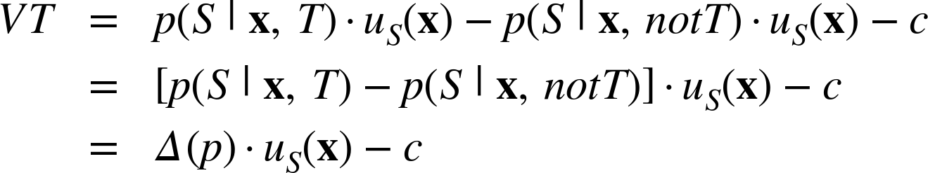
where ![]() is the difference in the predicted
probabilities of staying, depending on whether the customer is targeted or
not. Again we see an intuitive result: we want to target those customers with
the greatest change in their probability of staying, moderated by their value
if they were to stay! In other words, target those with the greatest change
in their expected value as a result of targeting. (The -c is the same for
everyone in our scenario, and including it here simply assures that the VT
is not expected to be a monetary loss.)
is the difference in the predicted
probabilities of staying, depending on whether the customer is targeted or
not. Again we see an intuitive result: we want to target those customers with
the greatest change in their probability of staying, moderated by their value
if they were to stay! In other words, target those with the greatest change
in their expected value as a result of targeting. (The -c is the same for
everyone in our scenario, and including it here simply assures that the VT
is not expected to be a monetary loss.)
It’s important not to lose track: this was all work in our Business Understanding phase. Let’s turn to the implications for the rest of the data mining process.
From an Expected Value Decomposition to a Data Science Solution
The prior discussion and specifically the decomposition highlighted in
Equation 11-1 guide us in our data understanding, data formulation,
modeling, and evaluation. In particular, from the decomposition we can see
precisely what models we will want to build: models to estimate
![]() and
and
![]() , the probability that a customer
will stay if targeted and the probability that a customer will stay anyway,
even if not targeted. Unlike our prior data mining solutions, here we want to
build two separate probability estimation models. Once these models are
built, we can use them to compute the expected value of targeting.
, the probability that a customer
will stay if targeted and the probability that a customer will stay anyway,
even if not targeted. Unlike our prior data mining solutions, here we want to
build two separate probability estimation models. Once these models are
built, we can use them to compute the expected value of targeting.
Importantly, the expected value decomposition focuses our Data Understanding efforts. What data do we need to build these models? In both cases, we need samples of customers who have reached contract expiration. Indeed, we need samples of customers who have gone far enough beyond contract expiration that we are satisfied with concluding they have definitely “stayed” or “left.” For the first model we need a sample of customers who were targeted with the offer. For the second model, we need a sample of customers who were not targeted with the offer. Hopefully this would be a representative sample of the customer base to which the model was applied (see the above discussion of selection bias). Developing our Data Understanding, let’s think more deeply about each of these in turn.
How can we obtain a sample of such customers who have not been targeted with the offer? First, we should assure ourselves that nothing substantial has changed in the business environment that would call into question the use of historical data for churn prediction (e.g., the introduction of the iPhone only to AT&T customers would have been such an event for the other phone companies). Assuming there has been no such event, gathering the requisite data should be relatively straightforward: the phone company keeps substantial data on customers for many months, for billing, fraud detection, and other purposes. Given that this is a new offer, none of them would have been targeted with it. We would want to double-check that none of our customers was made some other offer that would affect the likelihood of churning.
The situation with modeling ![]() is quite
different, and again highlights how the expected value framework can focus our
thinking early, highlighting issues and challenges that we face. What’s the
challenge here? This is a new offer. No one has seen it yet. We do not have
the data to build a model to estimate
is quite
different, and again highlights how the expected value framework can focus our
thinking early, highlighting issues and challenges that we face. What’s the
challenge here? This is a new offer. No one has seen it yet. We do not have
the data to build a model to estimate ![]() !
!
Nonetheless, business exigencies may force us to proceed. We need to reduce churn; Marketing has confidence in this offer, and we certainly have some data that might inform how we proceed. This is not an uncommon situation in the application of data science to solving a real business problem. The expected value decomposition can lead us to a complex formulation that helps us to understand the problem, but for which we are not willing or able to address the full complexity. It may be that we simply do not have the resources (data, human, or computing). In our churn example, we do not have the data necessary.
A different scenario might be that we do not believe that the added complexity
of the full formulation will add substantially to our effectiveness. For
example, we might conclude, “Yes, the formulation of
Equation 11-1 helps me understand what I should do, but I believe I
will do just about as well with a simpler or cheaper formulation.” For
example, what if we were to assume that when given the offer, everyone would
Stay with certainty, ![]() ? This is obviously an
oversimplification, but it may allow us to act—and in business we need to be
ready to act even without ideal information. You could verify via
Equation 11-1 that the result of applying this assumption would be
simply to target those customers with the largest
? This is obviously an
oversimplification, but it may allow us to act—and in business we need to be
ready to act even without ideal information. You could verify via
Equation 11-1 that the result of applying this assumption would be
simply to target those customers with the largest ![]() —
i.e., the customers with the largest expected loss if they were to leave.
That makes a lot of sense if we do not have data on the actual differential
effect of the offer.
—
i.e., the customers with the largest expected loss if they were to leave.
That makes a lot of sense if we do not have data on the actual differential
effect of the offer.
Consider an alternative course of action in a case such as this, where sufficient data are not available on a modeling target. One can instead label the data with a “proxy” for the target label of interest. For example, perhaps Marketing had come up with a similar, but not identical, offer in the past. If this offer had been made to customers in a similar situation (and recall the selection bias concern discussed above), it may be useful to build a model using the proxy label.[66]
The expected value decomposition highlights yet
another option. What would we need to do to model
![]() ? We need to obtain data.
Specifically, we need to obtain data for customers who are targeted. That
means we have to target customers. However, this would incur a cost. What if
we target poorly and waste money targeting customers with lower probabilities
of responding? This situation relates back to our very first fundamental
principle of data science: data should be treated as an asset. We need to think not only about
taking advantage of the assets that we already have, but also about investing
in data assets from which we can generate important returns. Recall from Chapter 1 the situation Signet Bank faced in
Data and Data Science Capability as a Strategic Asset. They did not have data on the differential
response of customers to the various new sorts of offers they had designed.
So they invested in data, taking losses by making offers broadly, and the data assets they acquired are considered to be the reason they
became the wildly successful Capital One. Our situation may not be so grand,
in that we have a single offer, and in making the offer we are not likely to
lose the sort of money that Signet Bank did when their customers defaulted.
Nonetheless, the lesson is the same: if we are willing to invest in data on
how people will respond to this offer, we may be able to better target the
offer to future customers.
? We need to obtain data.
Specifically, we need to obtain data for customers who are targeted. That
means we have to target customers. However, this would incur a cost. What if
we target poorly and waste money targeting customers with lower probabilities
of responding? This situation relates back to our very first fundamental
principle of data science: data should be treated as an asset. We need to think not only about
taking advantage of the assets that we already have, but also about investing
in data assets from which we can generate important returns. Recall from Chapter 1 the situation Signet Bank faced in
Data and Data Science Capability as a Strategic Asset. They did not have data on the differential
response of customers to the various new sorts of offers they had designed.
So they invested in data, taking losses by making offers broadly, and the data assets they acquired are considered to be the reason they
became the wildly successful Capital One. Our situation may not be so grand,
in that we have a single offer, and in making the offer we are not likely to
lose the sort of money that Signet Bank did when their customers defaulted.
Nonetheless, the lesson is the same: if we are willing to invest in data on
how people will respond to this offer, we may be able to better target the
offer to future customers.
Note
It’s worth reiterating the importance of deep business understanding. Depending on the structure of the offer, we may not lose that much if the offer is not taken, so the simpler formulation above may be quite satisfactory.
Note that this investment in data can be managed carefully, also applying conceptual tools developed through the book. Recall the notion of visualizing performance via the learning curve, from Chapter 8. The learning curve helps us to understand the relationship between the amount of data—in this case, the amount of investment in data so far—and the resultant improvement in generalization performance. We can easily extend the notion of generalization performance to include the improvement in performance over a baseline (recall our fundamental concept: think carefully about what you will compare to). That baseline could be our alternative, simple churn model. Thus, we would slowly invest in data, examining whether increasing our data is improving our performance, and whether extrapolating the curve indicates that there are more improvements to come. If this analysis suggests that the investment is not worthwhile, it can be aborted.
Importantly, that does not mean the investment was wasteful. We invested in information: here, information about whether the additional data would pay off for our ultimate task of cost-effective churn reduction.
Furthermore, framing the problem using expected value allows extensions to the formulation to provide a structured way to approach the question of: what is the right offer to give. We could expand the formulation to include multiple offers, and judge which gives the best value for any particular customer. Or we could parameterize the offers (for example with a variable discount amount) and then work to optimize what discount will yield the best expected value. This would likely involve additional investment in data, running experiments to judge different customers’ probabilities of staying or leaving at different offer levels—again similar to what Signet Bank did in becoming Capital One.
Summary
By following through the donation and churn examples, we have seen how the expected value framework can help articulate the true business problem and the role(s) data mining will play in its solution.
It is possible to keep elaborating the business problem into greater and greater detail, uncovering additional complexity in the problem (and greater demands on its solution). You may wonder, “Where does this all end? Can’t I keep pushing the analysis on forever?” In principle, yes, but modeling always involves making some simplifying assumptions to keep the problem tractable. There will always be points in analytical engineering at which you should conclude:
- We can’t get data on this event,
- It would be too expensive to model this aspect accurately,
- This event is so improbable we’re just going to ignore it, or
- This formulation seems sufficient for the time being, and we should proceed with it.
The point of analytical engineering is not to develop complex solutions by addressing every possible contingency. Rather, the point is to promote thinking about problems data analytically so that the role of data mining is clear, the business constraints, cost, and benefits are considered, and any simplifying assumptions are made consciously and explicitly. This increases the chance of project success and reduces the risk of being blindsided by problems during deployment.
[65] This also is an essential starting point for causal analysis: create a so-called counterfactual situation assessing the difference in expected values between two otherwise identical settings. These settings are often called the “treated” and “untreated” cases, in analogy to medical inference, where one often wants to assess the causal influence of the treatment. The many different frameworks for causal analysis, from randomized experimentation, to regression-based causal analysis, to more modern causal modeling approaches, all have this difference in expected values at their core. We will discuss causal data analysis further in Chapter 12.
[66] For some applications, proxy labels might come from completely different events from the event on which the actual target label is based. For example, for building models to predict who will purchase after being targeted with an advertisement, data on actual conversions are scarce. It is surprisingly effective to use visiting the campaign’s brand’s website as a modeling proxy for purchasing (Dalessandro, Hook, Perlich, & Provost, 2012).