Chapter 2. Business Problems and Data Science Solutions
Fundamental concepts: A set of canonical data mining tasks; The data mining process; Supervised versus unsupervised data mining.
An important principle of data science is that data mining is a process with fairly well-understood stages. Some involve the application of information technology, such as the automated discovery and evaluation of patterns from data, while others mostly require an analyst’s creativity, business knowledge, and common sense. Understanding the whole process helps to structure data mining projects, so they are closer to systematic analyses rather than heroic endeavors driven by chance and individual acumen.
Since the data mining process breaks up the overall task of finding patterns from data into a set of well-defined subtasks, it is also useful for structuring discussions about data science. In this book, we will use the process as an overarching framework for our discussion. This chapter introduces the data mining process, but first we provide additional context by discussing common types of data mining tasks. Introducing these allows us to be more concrete when presenting the overall process, as well as when introducing other concepts in subsequent chapters.
We close the chapter by discussing a set of important business analytics subjects that are not the focus of this book (but for which there are many other helpful books), such as databases, data warehousing, and basic statistics.
From Business Problems to Data Mining Tasks
Each data-driven business decision-making problem is unique, comprising its own combination of goals, desires, constraints, and even personalities. As with much engineering, though, there are sets of common tasks that underlie the business problems. In collaboration with business stakeholders, data scientists decompose a business problem into subtasks. The solutions to the subtasks can then be composed to solve the overall problem. Some of these subtasks are unique to the particular business problem, but others are common data mining tasks. For example, our telecommunications churn problem is unique to MegaTelCo: there are specifics of the problem that are different from churn problems of any other telecommunications firm. However, a subtask that will likely be part of the solution to any churn problem is to estimate from historical data the probability of a customer terminating her contract shortly after it has expired. Once the idiosyncratic MegaTelCo data have been assembled into a particular format (described in the next chapter), this probability estimation fits the mold of one very common data mining task. We know a lot about solving the common data mining tasks, both scientifically and practically. In later chapters, we also will provide data science frameworks to help with the decomposition of business problems and with the re-composition of the solutions to the subtasks.
Tip
A critical skill in data science is the ability to decompose a data-analytics problem into pieces such that each piece matches a known task for which tools are available. Recognizing familiar problems and their solutions avoids wasting time and resources reinventing the wheel. It also allows people to focus attention on more interesting parts of the process that require human involvement—parts that have not been automated, so human creativity and intelligence must come into play.
Despite the large number of specific data mining algorithms developed over the years, there are only a handful of fundamentally different types of tasks these algorithms address. It is worth defining these tasks clearly. The next several chapters will use the first two (classification and regression) to illustrate several fundamental concepts. In what follows, the term “an individual” will refer to an entity about which we have data, such as a customer or a consumer, or it could be an inanimate entity such as a business. We will make this notion more precise in Chapter 3. In many business analytics projects, we want to find “correlations” between a particular variable describing an individual and other variables. For example, in historical data we may know which customers left the company after their contracts expired. We may want to find out which other variables correlate with a customer leaving in the near future. Finding such correlations are the most basic examples of classification and regression tasks.
Classification and class probability estimation attempt to predict, for each individual in a population, which of a (small) set of classes this individual belongs to. Usually the classes are mutually exclusive. An example classification question would be: “Among all the customers of MegaTelCo, which are likely to respond to a given offer?” In this example the two classes could be called
will respondandwill not respond.For a classification task, a data mining procedure produces a model that, given a new individual, determines which class that individual belongs to. A closely related task is scoring or class probability estimation. A scoring model applied to an individual produces, instead of a class prediction, a score representing the probability (or some other quantification of likelihood) that that individual belongs to each class. In our customer response scenario, a scoring model would be able to evaluate each individual customer and produce a score of how likely each is to respond to the offer. Classification and scoring are very closely related; as we shall see, a model that can do one can usually be modified to do the other.
Regression (“value estimation”) attempts to estimate or predict, for each individual, the numerical value of some variable for that individual. An example regression question would be: “How much will a given customer use the service?” The property (variable) to be predicted here is service usage, and a model could be generated by looking at other, similar individuals in the population and their historical usage. A regression procedure produces a model that, given an individual, estimates the value of the particular variable specific to that individual.
Regression is related to classification, but the two are different. Informally, classification predicts whether something will happen, whereas regression predicts how much something will happen. The difference will become clearer as the book progresses.
- Similarity matching attempts to identify similar individuals based on data known about them. Similarity matching can be used directly to find similar entities. For example, IBM is interested in finding companies similar to their best business customers, in order to focus their sales force on the best opportunities. They use similarity matching based on “firmographic” data describing characteristics of the companies. Similarity matching is the basis for one of the most popular methods for making product recommendations (finding people who are similar to you in terms of the products they have liked or have purchased). Similarity measures underlie certain solutions to other data mining tasks, such as classification, regression, and clustering. We discuss similarity and its uses at length in Chapter 6.
- Clustering attempts to group individuals in a population together by their similarity, but not driven by any specific purpose. An example clustering question would be: “Do our customers form natural groups or segments?” Clustering is useful in preliminary domain exploration to see which natural groups exist because these groups in turn may suggest other data mining tasks or approaches. Clustering also is used as input to decision-making processes focusing on questions such as: What products should we offer or develop? How should our customer care teams (or sales teams) be structured? We discuss clustering in depth in Chapter 6.
Co-occurrence grouping (also known as frequent itemset mining, association rule discovery, and market-basket analysis) attempts to find associations between entities based on transactions involving them. An example co-occurrence question would be: What items are commonly purchased together? While clustering looks at similarity between objects based on the objects’ attributes, co-occurrence grouping considers similarity of objects based on their appearing together in transactions. For example, analyzing purchase records from a supermarket may uncover that ground meat is purchased together with hot sauce much more frequently than we might expect. Deciding how to act upon this discovery might require some creativity, but it could suggest a special promotion, product display, or combination offer. Co-occurrence of products in purchases is a common type of grouping known as market-basket analysis. Some recommendation systems also perform a type of affinity grouping by finding, for example, pairs of books that are purchased frequently by the same people (“people who bought X also bought Y”).
The result of co-occurrence grouping is a description of items that occur together. These descriptions usually include statistics on the frequency of the co-occurrence and an estimate of how surprising it is.
Profiling (also known as behavior description) attempts to characterize the typical behavior of an individual, group, or population. An example profiling question would be: “What is the typical cell phone usage of this customer segment?” Behavior may not have a simple description; profiling cell phone usage might require a complex description of night and weekend airtime averages, international usage, roaming charges, text minutes, and so on. Behavior can be described generally over an entire population, or down to the level of small groups or even individuals.
Profiling is often used to establish behavioral norms for anomaly detection applications such as fraud detection and monitoring for intrusions to computer systems (such as someone breaking into your iTunes account). For example, if we know what kind of purchases a person typically makes on a credit card, we can determine whether a new charge on the card fits that profile or not. We can use the degree of mismatch as a suspicion score and issue an alarm if it is too high.
- Link prediction attempts to predict connections between data items, usually by suggesting that a link should exist, and possibly also estimating the strength of the link. Link prediction is common in social networking systems: “Since you and Karen share 10 friends, maybe you’d like to be Karen’s friend?” Link prediction can also estimate the strength of a link. For example, for recommending movies to customers one can think of a graph between customers and the movies they’ve watched or rated. Within the graph, we search for links that do not exist between customers and movies, but that we predict should exist and should be strong. These links form the basis for recommendations.
- Data reduction attempts to take a large set of data and replace it with a smaller set of data that contains much of the important information in the larger set. The smaller dataset may be easier to deal with or to process. Moreover, the smaller dataset may better reveal the information. For example, a massive dataset on consumer movie-viewing preferences may be reduced to a much smaller dataset revealing the consumer taste preferences that are latent in the viewing data (for example, viewer genre preferences). Data reduction usually involves loss of information. What is important is the trade-off for improved insight.
Causal modeling attempts to help us understand what events or actions actually influence others. For example, consider that we use predictive modeling to target advertisements to consumers, and we observe that indeed the targeted consumers purchase at a higher rate subsequent to having been targeted. Was this because the advertisements influenced the consumers to purchase? Or did the predictive models simply do a good job of identifying those consumers who would have purchased anyway? Techniques for causal modeling include those involving a substantial investment in data, such as randomized controlled experiments (e.g., so-called “A/B tests”), as well as sophisticated methods for drawing causal conclusions from observational data. Both experimental and observational methods for causal modeling generally can be viewed as “counterfactual” analysis: they attempt to understand what would be the difference between the situations—which cannot both happen—where the “treatment” event (e.g., showing an advertisement to a particular individual) were to happen, and were not to happen.
In all cases, a careful data scientist should always include with a causal conclusion the exact assumptions that must be made in order for the causal conclusion to hold (there always are such assumptions—always ask). When undertaking causal modeling, a business needs to weigh the trade-off of increasing investment to reduce the assumptions made, versus deciding that the conclusions are good enough given the assumptions. Even in the most careful randomized, controlled experimentation, assumptions are made that could render the causal conclusions invalid. The discovery of the “placebo effect” in medicine illustrates a notorious situation where an assumption was overlooked in carefully designed randomized experimentation.
Discussing all of these tasks in detail would fill multiple books. In this book, we present a collection of the most fundamental data science principles—principles that together underlie all of these types of tasks. We will illustrate the principles mainly using classification, regression, similarity matching, and clustering, and will discuss others when they provide important illustrations of the fundamental principles (toward the end of the book).
Consider which of these types of tasks might fit our churn-prediction problem. Often, practitioners formulate churn prediction as a problem of finding segments of customers who are more or less likely to leave. This segmentation problem sounds like a classification problem, or possibly clustering, or even regression. To decide the best formulation, we first need to introduce some important distinctions.
Supervised Versus Unsupervised Methods
Consider two similar questions we might ask about a customer population. The first is: “Do our customers naturally fall into different groups?” Here no specific purpose or target has been specified for the grouping. When there is no such target, the data mining problem is referred to as unsupervised. Contrast this with a slightly different question: “Can we find groups of customers who have particularly high likelihoods of canceling their service soon after their contracts expire?” Here there is a specific target defined: will a customer leave when her contract expires? In this case, segmentation is being done for a specific reason: to take action based on likelihood of churn. This is called a supervised data mining problem.
A note on the terms: Supervised and unsupervised learning
The terms supervised and unsupervised were inherited from the field of machine learning. Metaphorically, a teacher “supervises” the learner by carefully providing target information along with a set of examples. An unsupervised learning task might involve the same set of examples but would not include the target information. The learner would be given no information about the purpose of the learning, but would be left to form its own conclusions about what the examples have in common.
The difference between these questions is subtle but important. If a specific target can be provided, the problem can be phrased as a supervised one. Supervised tasks require different techniques than unsupervised tasks do, and the results often are much more useful. A supervised technique is given a specific purpose for the grouping—predicting the target. Clustering, an unsupervised task, produces groupings based on similarities, but there is no guarantee that these similarities are meaningful or will be useful for any particular purpose.
Technically, another condition must be met for supervised data mining: there must be data on the target. It is not enough that the target information exist in principle; it must also exist in the data. For example, it might be useful to know whether a given customer will stay for at least six months, but if in historical data this retention information is missing or incomplete (if, say, the data are only retained for two months) the target values cannot be provided. Acquiring data on the target often is a key data science investment. The value for the target variable for an individual is often called the individual’s label, emphasizing that often (not always) one must incur expense to actively label the data.
Classification, regression, and causal modeling generally are solved with supervised methods. Similarity matching, link prediction, and data reduction could be either. Clustering, co-occurrence grouping, and profiling generally are unsupervised. The fundamental principles of data mining that we will present underlie all these types of technique.
Two main subclasses of supervised data mining, classification and regression, are distinguished by the type of target. Regression involves a numeric target while classification involves a categorical (often binary) target. Consider these similar questions we might address with supervised data mining:
- “Will this customer purchase service S1 if given incentive I?”
- This is a classification problem because it has a binary target (the customer either purchases or does not).
- “Which service package (S1, S2, or none) will a customer likely purchase if given incentive I?”
- This is also a classification problem, with a three-valued target.
- “How much will this customer use the service?”
- This is a regression problem because it has a numeric target. The target variable is the amount of usage (actual or predicted) per customer.
There are subtleties among these questions that should be brought out. For business applications we often want a numerical prediction over a categorical target. In the churn example, a basic yes/no prediction of whether a customer is likely to continue to subscribe to the service may not be sufficient; we want to model the probability that the customer will continue. This is still considered classification modeling rather than regression because the underlying target is categorical. Where necessary for clarity, this is called “class probability estimation.”
A vital part in the early stages of the data mining process is (i) to decide whether the line of attack will be supervised or unsupervised, and (ii) if supervised, to produce a precise definition of a target variable. This variable must be a specific quantity that will be the focus of the data mining (and for which we can obtain values for some example data). We will return to this in Chapter 3.

Data Mining and Its Results
There is another important distinction pertaining to mining data: the difference between (1) mining the data to find patterns and build models, and (2) using the results of data mining. Students often confuse these two processes when studying data science, and managers sometimes confuse them when discussing business analytics. The use of data mining results should influence and inform the data mining process itself, but the two should be kept distinct.
In our churn example, consider the deployment scenario in which the results will be used. We want to use the model to predict which of our customers will leave. Specifically, assume that data mining has created a class probability estimation model M. Given each existing customer, described using a set of characteristics, M takes these characteristics as input and produces a score or probability estimate of attrition. This is the use of the results of data mining. The data mining produces the model M from some other, often historical, data.
Figure 2-1 illustrates these two phases. Data mining produces the probability estimation model, as shown in the top half of the figure. In the use phase (bottom half), the model is applied to a new, unseen case and it generates a probability estimate for it.
The Data Mining Process
Data mining is a craft. It involves the application of a substantial amount of science and technology, but the proper application still involves art as well. But as with many mature crafts, there is a well-understood process that places a structure on the problem, allowing reasonable consistency, repeatability, and objectiveness. A useful codification of the data mining process is given by the Cross Industry Standard Process for Data Mining (CRISP-DM; Shearer, 2000), illustrated in Figure 2-2.[7]
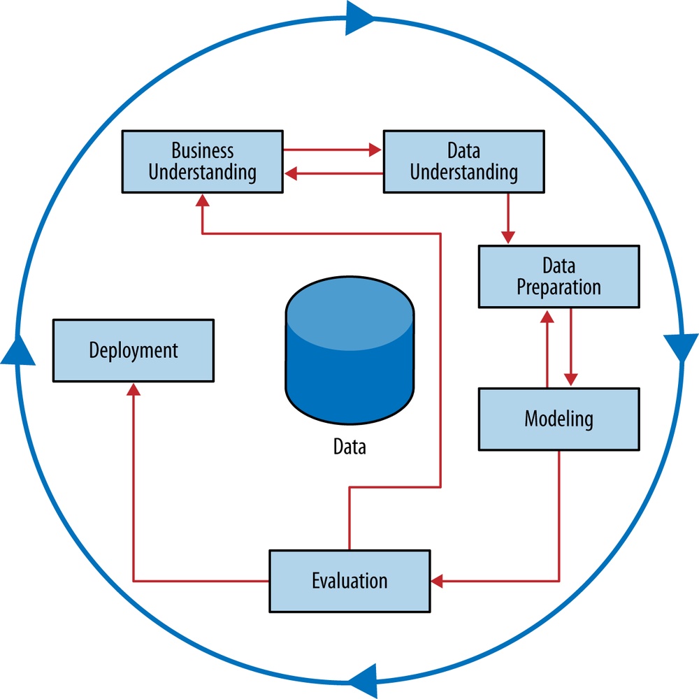
This process diagram makes explicit the fact that iteration is the rule rather than the exception. Going through the process once without having solved the problem is, generally speaking, not a failure. Often the entire process is an exploration of the data, and after the first iteration the data science team knows much more. The next iteration can be much more well-informed. Let’s now discuss the steps in detail.
Business Understanding
Initially, it is vital to understand the problem to be solved. This may seem obvious, but business projects seldom come pre-packaged as clear and unambiguous data mining problems. Often recasting the problem and designing a solution is an iterative process of discovery. The diagram shown in Figure 2-2 represents this as cycles within a cycle, rather than as a simple linear process. The initial formulation may not be complete or optimal so multiple iterations may be necessary for an acceptable solution formulation to appear.
The Business Understanding stage represents a part of the craft where the analysts’ creativity plays a large role. Data science has some things to say, as we will describe, but often the key to a great success is a creative problem formulation by some analyst regarding how to cast the business problem as one or more data science problems. High-level knowledge of the fundamentals helps creative business analysts see novel formulations.
We have a set of powerful tools to solve particular data mining problems: the basic data mining tasks discussed in From Business Problems to Data Mining Tasks. Typically, the early stages of the endeavor involve designing a solution that takes advantage of these tools. This can mean structuring (engineering) the problem such that one or more subproblems involve building models for classification, regression, probability estimation, and so on.
In this first stage, the design team should think carefully about the problem to be solved and about the use scenario. This itself is one of the most important fundamental principles of data science, to which we have devoted two entire chapters (Chapter 7 and Chapter 11). What exactly do we want to do? How exactly would we do it? What parts of this use scenario constitute possible data mining models? In discussing this in more detail, we will begin with a simplified view of the use scenario, but as we go forward we will loop back and realize that often the use scenario must be adjusted to better reflect the actual business need. We will present conceptual tools to help our thinking here, for example framing a business problem in terms of expected value can allow us to systematically decompose it into data mining tasks.
Data Understanding
If solving the business problem is the goal, the data comprise the available raw material from which the solution will be built. It is important to understand the strengths and limitations of the data because rarely is there an exact match with the problem. Historical data often are collected for purposes unrelated to the current business problem, or for no explicit purpose at all. A customer database, a transaction database, and a marketing response database contain different information, may cover different intersecting populations, and may have varying degrees of reliability.
It is also common for the costs of data to vary. Some data will be available virtually for free while others will require effort to obtain. Some data may be purchased. Still other data simply won’t exist and will require entire ancillary projects to arrange their collection. A critical part of the data understanding phase is estimating the costs and benefits of each data source and deciding whether further investment is merited. Even after all datasets are acquired, collating them may require additional effort. For example, customer records and product identifiers are notoriously variable and noisy. Cleaning and matching customer records to ensure only one record per customer is itself a complicated analytics problem (Hernández & Stolfo, 1995; Elmagarmid, Ipeirotis, & Verykios, 2007).
As data understanding progresses, solution paths may change direction in response, and team efforts may even fork. Fraud detection provides an illustration of this. Data mining has been used extensively for fraud detection, and many fraud detection problems involve classic supervised data mining tasks. Consider the task of catching credit card fraud. Charges show up on each customer’s account, so fraudulent charges are usually caught—if not initially by the company, then later by the customer when account activity is reviewed. We can assume that nearly all fraud is identified and reliably labeled, since the legitimate customer and the person perpetrating the fraud are different people and have opposite goals. Thus credit card transactions have reliable labels (fraud and legitimate) that may serve as targets for a supervised technique.
Now consider the related problem of catching Medicare fraud. This is a huge problem in the United States costing billions of dollars annually. Though this may seem like a conventional fraud detection problem, as we consider the relationship of the business problem to the data, we realize that the problem is significantly different. The perpetrators of fraud—medical providers who submit false claims, and sometimes their patients—are also legitimate service providers and users of the billing system. Those who commit fraud are a subset of the legitimate users; there is no separate disinterested party who will declare exactly what the “correct” charges should be. Consequently the Medicare billing data have no reliable target variable indicating fraud, and a supervised learning approach that could work for credit card fraud is not applicable. Such a problem usually requires unsupervised approaches such as profiling, clustering, anomaly detection, and co-occurrence grouping.
The fact that both of these are fraud detection problems is a superficial similarity that is actually misleading. In data understanding we need to dig beneath the surface to uncover the structure of the business problem and the data that are available, and then match them to one or more data mining tasks for which we may have substantial science and technology to apply. It is not unusual for a business problem to contain several data mining tasks, often of different types, and combining their solutions will be necessary (see Chapter 11).
Data Preparation
The analytic technologies that we can bring to bear are powerful but they impose certain requirements on the data they use. They often require data to be in a form different from how the data are provided naturally, and some conversion will be necessary. Therefore a data preparation phase often proceeds along with data understanding, in which the data are manipulated and converted into forms that yield better results.
Typical examples of data preparation are converting data to tabular format, removing or inferring missing values, and converting data to different types. Some data mining techniques are designed for symbolic and categorical data, while others handle only numeric values. In addition, numerical values must often be normalized or scaled so that they are comparable. Standard techniques and rules of thumb are available for doing such conversions. Chapter 3 discusses the most typical format for mining data in some detail.
In general, though, this book will not focus on data preparation techniques, which could be the topic of a book by themselves (Pyle, 1999). We will define basic data formats in following chapters, and will only be concerned with data preparation details when they shed light on some fundamental principle of data science or are necessary to present a concrete example.
Note
More generally, data scientists may spend considerable time early in the process defining the variables used later in the process. This is one of the main points at which human creativity, common sense, and business knowledge come into play. Often the quality of the data mining solution rests on how well the analysts structure the problems and craft the variables (and sometimes it can be surprisingly hard for them to admit it).
One very general and important concern during data preparation is to beware of “leaks” (Kaufman et al. 2012). A leak is a situation where a variable collected in historical data gives information on the target variable—information that appears in historical data but is not actually available when the decision has to be made. As an example, when predicting whether at a particular point in time a website visitor would end her session or continue surfing to another page, the variable “total number of webpages visited in the session” is predictive. However, the total number of webpages visited in the session would not be known until after the session was over (Kohavi et al., 2000)—at which point one would know the value for the target variable! As another illustrative example, consider predicting whether a customer will be a “big spender”; knowing the categories of the items purchased (or worse, the amount of tax paid) are very predictive, but are not known at decision-making time (Kohavi & Parekh, 2003). Leakage must be considered carefully during data preparation, because data preparation typically is performed after the fact—from historical data. We present a more detailed example of a real leak that was challenging to find in Chapter 14.
Modeling
Modeling is the subject of the next several chapters and we will not dwell on it here, except to say that the output of modeling is some sort of model or pattern capturing regularities in the data.
The modeling stage is the primary place where data mining techniques are applied to the data. It is important to have some understanding of the fundamental ideas of data mining, including the sorts of techniques and algorithms that exist, because this is the part of the craft where the most science and technology can be brought to bear.
Evaluation
The purpose of the evaluation stage is to assess the data mining results rigorously and to gain confidence that they are valid and reliable before moving on. If we look hard enough at any dataset we will find patterns, but they may not survive careful scrutiny. We would like to have confidence that the models and patterns extracted from the data are true regularities and not just idiosyncrasies or sample anomalies. It is possible to deploy results immediately after data mining but this is inadvisable; it is usually far easier, cheaper, quicker, and safer to test a model first in a controlled laboratory setting.
Equally important, the evaluation stage also serves to help ensure that the model satisfies the original business goals. Recall that the primary goal of data science for business is to support decision making, and that we started the process by focusing on the business problem we would like to solve. Usually a data mining solution is only a piece of the larger solution, and it needs to be evaluated as such. Further, even if a model passes strict evaluation tests in “in the lab,” there may be external considerations that make it impractical. For example, a common flaw with detection solutions (such as fraud detection, spam detection, and intrusion monitoring) is that they produce too many false alarms. A model may be extremely accurate (> 99%) by laboratory standards, but evaluation in the actual business context may reveal that it still produces too many false alarms to be economically feasible. (How much would it cost to provide the staff to deal with all those false alarms? What would be the cost in customer dissatisfaction?)
Evaluating the results of data mining includes both quantitative and qualitative assessments. Various stakeholders have interests in the business decision-making that will be accomplished or supported by the resultant models. In many cases, these stakeholders need to “sign off” on the deployment of the models, and in order to do so need to be satisfied by the quality of the model’s decisions. What that means varies from application to application, but often stakeholders are looking to see whether the model is going to do more good than harm, and especially that the model is unlikely to make catastrophic mistakes.[8] To facilitate such qualitative assessment, the data scientist must think about the comprehensibility of the model to stakeholders (not just to the data scientists). And if the model itself is not comprehensible (e.g., maybe the model is a very complex mathematical formula), how can the data scientists work to make the behavior of the model be comprehensible.
Finally, a comprehensive evaluation framework is important because getting detailed information on the performance of a deployed model may be difficult or impossible. Often there is only limited access to the deployment environment so making a comprehensive evaluation “in production” is difficult. Deployed systems typically contain many “moving parts,” and assessing the contribution of a single part is difficult. Firms with sophisticated data science teams wisely build testbed environments that mirror production data as closely as possible, in order to get the most realistic evaluations before taking the risk of deployment.
Nonetheless, in some cases we may want to extend evaluation into the development environment, for example by instrumenting a live system to be able to conduct randomized experiments. In our churn example, if we have decided from laboratory tests that a data mined model will give us better churn reduction, we may want to move on to an “in vivo” evaluation, in which a live system randomly applies the model to some customers while keeping other customers as a control group (recall our discussion of causal modeling from Chapter 1). Such experiments must be designed carefully, and the technical details are beyond the scope of this book. The interested reader could start with the lessons-learned articles by Ron Kohavi and his coauthors (Kohavi et al., 2007, 2009, 2012). We may also want to instrument deployed systems for evaluations to make sure that the world is not changing to the detriment of the model’s decision-making. For example, behavior can change—in some cases, like fraud or spam, in direct response to the deployment of models. Additionally, the output of the model is critically dependent on the input data; input data can change in format and in substance, often without any alerting of the data science team. Raeder et al. (2012) present a detailed discussion of system design to help deal with these and other related evaluation-in-deployment issues.
Deployment
In deployment the results of data mining—and increasingly the data mining techniques themselves—are put into real use in order to realize some return on investment. The clearest cases of deployment involve implementing a predictive model in some information system or business process. In our churn example, a model for predicting the likelihood of churn could be integrated with the business process for churn management—for example, by sending special offers to customers who are predicted to be particularly at risk. (We will discuss this in increasing detail as the book proceeds.) A new fraud detection model may be built into a workforce management information system, to monitor accounts and create “cases” for fraud analysts to examine.
Increasingly, the data mining techniques themselves are deployed. For example, for targeting online advertisements, systems are deployed that automatically build (and test) models in production when a new advertising campaign is presented. Two main reasons for deploying the data mining system itself rather than the models produced by a data mining system are (i) the world may change faster than the data science team can adapt, as with fraud and intrusion detection, and (ii) a business has too many modeling tasks for their data science team to manually curate each model individually. In these cases, it may be best to deploy the data mining phase into production. In doing so, it is critical to instrument the process to alert the data science team of any seeming anomalies and to provide fail-safe operation (Raeder et al., 2012).
Note
Deployment can also be much less “technical.” In a celebrated case, data mining discovered a set of rules that could help to quickly diagnose and fix a common error in industrial printing. The deployment succeeded simply by taping a sheet of paper containing the rules to the side of the printers (Evans & Fisher, 2002). Deployment can also be much more subtle, such as a change to data acquisition procedures, or a change to strategy, marketing, or operations resulting from insight gained from mining the data.
Deploying a model into a production system typically requires that the model be re-coded for the production environment, usually for greater speed or compatibility with an existing system. This may incur substantial expense and investment. In many cases, the data science team is responsible for producing a working prototype, along with its evaluation. These are passed to a development team.
Note
Practically speaking, there are risks with “over the wall” transfers from data science to development. It may be helpful to remember the maxim: “Your model is not what the data scientists design, it’s what the engineers build.” From a management perspective, it is advisable to have members of the development team involved early on in the data science project. They can begin as advisors, providing critical insight to the data science team. Increasingly in practice, these particular developers are “data science engineers”—software engineers who have particular expertise both in the production systems and in data science. These developers gradually assume more responsibility as the project matures. At some point the developers will take the lead and assume ownership of the product. Generally, the data scientists should still remain involved in the project into final deployment, as advisors or as developers depending on their skills.
Regardless of whether deployment is successful, the process often returns to the Business Understanding phase. The process of mining data produces a great deal of insight into the business problem and the difficulties of its solution. A second iteration can yield an improved solution. Just the experience of thinking about the business, the data, and the performance goals often leads to new ideas for improving business performance, and even new lines of business or new ventures.
Note that it is not necessary to fail in deployment to start the cycle again. The Evaluation stage may reveal that results are not good enough to deploy, and we need to adjust the problem definition or get different data. This is represented by the “shortcut” link from Evaluation back to Business Understanding in the process diagram. In practice, there should be shortcuts back from each stage to each prior one because the process always retains some exploratory aspects, and a project should be flexible enough to revisit prior steps based on discoveries made.[9]
Implications for Managing the Data Science Team
It is tempting—but usually a mistake—to view the data mining process as a software development cycle. Indeed, data mining projects are often treated and managed as engineering projects, which is understandable when they are initiated by software departments, with data generated by a large software system and analytics results fed back into it. Managers are usually familiar with software technologies and are comfortable managing software projects. Milestones can be agreed upon and success is usually unambiguous. Software managers might look at the CRISP data mining cycle (Figure 2-2) and think it looks comfortably similar to a software development cycle, so they should be right at home managing an analytics project the same way.
This can be a mistake because data mining is an exploratory undertaking closer to research and development than it is to engineering. The CRISP cycle is based around exploration; it iterates on approaches and strategy rather than on software designs. Outcomes are far less certain, and the results of a given step may change the fundamental understanding of the problem. Engineering a data mining solution directly for deployment can be an expensive premature commitment. Instead, analytics projects should prepare to invest in information to reduce uncertainty in various ways. Small investments can be made via pilot studies and throwaway prototypes. Data scientists should review the literature to see what else has been done and how it has worked. On a larger scale, a team can invest substantially in building experimental testbeds to allow extensive agile experimentation. If you’re a software manager, this will look more like research and exploration than you’re used to, and maybe more than you’re comfortable with.
Software skills versus analytics skills
Although data mining involves software, it also requires skills that may not be common among programmers. In software engineering, the ability to write efficient, high-quality code from requirements may be paramount. Team members may be evaluated using software metrics such as the amount of code written or number of bug tickets closed. In analytics, it’s more important for individuals to be able to formulate problems well, to prototype solutions quickly, to make reasonable assumptions in the face of ill-structured problems, to design experiments that represent good investments, and to analyze results. In building a data science team, these qualities, rather than traditional software engineering expertise, are skills that should be sought.
Other Analytics Techniques and Technologies
Business analytics involves the application of various technologies to the analysis of data. Many of these go beyond this book’s focus on data-analytic thinking and the principles of extracting useful patterns from data. Nonetheless, it is important to be acquainted with these related techniques, to understand what their goals are, what role they play, and when it may be beneficial to consult experts in them.
To this end, we present six groups of related analytic techniques. Where appropriate we draw comparisons and contrasts with data mining. The main difference is that data mining focuses on the automated search for knowledge, patterns, or regularities from data.[10] An important skill for a business analyst is to be able to recognize what sort of analytic technique is appropriate for addressing a particular problem.
Statistics
The term “statistics” has two different uses in business analytics. First, it is used as a catchall term for the computation of particular numeric values of interest from data (e.g., “We need to gather some statistics on our customers’ usage to determine what’s going wrong here.”) These values often include sums, averages, rates, and so on. Let’s call these “summary statistics.” Often we want to dig deeper, and calculate summary statistics conditionally on one or more subsets of the population (e.g., “Does the churn rate differ between male and female customers?” and “What about high-income customers in the Northeast (denotes a region of the USA)?”) Summary statistics are the basic building blocks of much data science theory and practice.
Summary statistics should be chosen with close attention to the business problem to be solved (one of the fundamental principles we will present later), and also with attention to the distribution of the data they are summarizing. For example, the average (mean) income in the United States according to the 2004 Census Bureau Economic Survey was over $60,000. If we were to use that as a measure of the average income in order to make policy decisions, we would be misleading ourselves. The distribution of incomes in the U.S. is highly skewed, with many people making relatively little and some people making fantastically much. In such cases, the arithmetic mean tells us relatively little about how much people are making. Instead, we should use a different measure of “average” income, such as the median. The median income—that amount where half the population makes more and half makes less—in the U.S. in the 2004 Census study was only $44,389—considerably less than the mean. This example may seem obvious because we are so accustomed to hearing about the “median income,” but the same reasoning applies to any computation of summary statistics: have you thought about the problem you would like to solve or the question you would like to answer? Have you considered the distribution of the data, and whether the chosen statistic is appropriate?
The other use of the term “statistics” is to denote the field of study that goes by that name, for which we might differentiate by using the proper name, Statistics. The field of Statistics provides us with a huge amount of knowledge that underlies analytics, and can be thought of as a component of the larger field of Data Science. For example, Statistics helps us to understand different data distributions and what statistics are appropriate to summarize each. Statistics helps us understand how to use data to test hypotheses and to estimate the uncertainty of conclusions. In relation to data mining, hypothesis testing can help determine whether an observed pattern is likely to be a valid, general regularity as opposed to a chance occurrence in some particular dataset. Most relevant to this book, many of the techniques for extracting models or patterns from data have their roots in Statistics.
For example, a preliminary study may suggest that customers in the Northeast have a churn rate of 22.5%, whereas the nationwide average churn rate is only 15%. This may be just a chance fluctuation since the churn rate is not constant; it varies over regions and over time, so differences are to be expected. But the Northeast rate is one and a half times the U.S. average, which seems unusually high. What is the chance that this is due to random variation? Statistical hypothesis testing is used to answer such questions.
Closely related is the quantification of uncertainty into confidence intervals. The overall churn rate is 15%, but there is some variation; traditional statistical analysis may reveal that 95% of the time the churn rate is expected to fall between 13% and 17%.
This contrasts with the (complementary) process of data mining, which may be seen as hypothesis generation. Can we find patterns in data in the first place? Hypothesis generation should then be followed by careful hypothesis testing (generally on different data; see Chapter 5). In addition, data mining procedures may produce numerical estimates, and we often also want to provide confidence intervals on these estimates. We will return to this when we discuss the evaluation of the results of data mining.
In this book we are not going to spend more time discussing these basic statistical concepts. There are plenty of introductory books on statistics and statistics for business, and any treatment we would try to squeeze in would be either very narrow or superficial.
That said, one statistical term that is often heard in the context of business analytics is “correlation.” For example, “Are there any indicators that correlate with a customer’s later defection?” As with the term statistics, “correlation” has both a general-purpose meaning (variations in one quantity tell us something about variations in the other), and a specific technical meaning (e.g., linear correlation based on a particular mathematical formula). The notion of correlation will be the jumping off point for the rest of our discussion of data science for business, starting in the next chapter.
Database Querying
A query is a specific request for a subset of data or for statistics about data, formulated in a technical language and posed to a database system. Many tools are available to answer one-off or repeating queries about data posed by an analyst. These tools are usually frontends to database systems, based on Structured Query Language (SQL) or a tool with a graphical user interface (GUI) to help formulate queries (e.g., query-by-example, or QBE). For example, if the analyst can define “profitable” in operational terms computable from items in the database, then a query tool could answer: “Who are the most profitable customers in the Northeast?” The analyst may then run the query to retrieve a list of the most profitable customers, possibly ranked by profitability. This activity differs fundamentally from data mining in that there is no discovery of patterns or models.
Database queries are appropriate when an analyst already has an idea of what might be an interesting subpopulation of the data, and wants to investigate this population or confirm a hypothesis about it. For example, if an analyst suspects that middle-aged men living in the Northeast have some particularly interesting churning behavior, she could compose a SQL query:
SELECT * FROM CUSTOMERS WHERE AGE > 45 and SEX='M' and DOMICILE = 'NE'
If those are the people to be targeted with an offer, a query tool can be used to retrieve all of the information about them (“*”) from the CUSTOMERS table in the database.
In contrast, data mining could be used to come up with this query in the first place—as a pattern or regularity in the data. A data mining procedure might examine prior customers who did and did not defect, and determine that this segment (characterized as “AGE is greater than 45 and SEX is male and DOMICILE is Northeast-USA”) is predictive with respect to churn rate. After translating this into a SQL query, a query tool could then be used to find the matching records in the database.
Query tools generally have the ability to execute sophisticated logic, including computing summary statistics over subpopulations, sorting, joining together multiple tables with related data, and more. Data scientists often become quite adept at writing queries to extract the data they need.
On-line Analytical Processing (OLAP) provides an easy-to-use GUI to query large data collections, for the purpose of facilitating data exploration. The idea of “on-line” processing is that it is done in realtime, so analysts and decision makers can find answers to their queries quickly and efficiently. Unlike the “ad hoc” querying enabled by tools like SQL, for OLAP the dimensions of analysis must be pre-programmed into the OLAP system. If we’ve foreseen that we would want to explore sales volume by region and time, we could have these three dimensions programmed into the system, and drill down into populations, often simply by clicking and dragging and manipulating dynamic charts.
OLAP systems are designed to facilitate manual or visual exploration of the data by analysts. OLAP performs no modeling or automatic pattern finding. As an additional contrast, unlike with OLAP, data mining tools generally can incorporate new dimensions of analysis easily as part of the exploration. OLAP tools can be a useful complement to data mining tools for discovery from business data.
Data Warehousing
Data warehouses collect and coalesce data from across an enterprise, often from multiple transaction-processing systems, each with its own database. Analytical systems can access data warehouses. Data warehousing may be seen as a facilitating technology of data mining. It is not always necessary, as most data mining does not access a data warehouse, but firms that decide to invest in data warehouses often can apply data mining more broadly and more deeply in the organization. For example, if a data warehouse integrates records from sales and billing as well as from human resources, it can be used to find characteristic patterns of effective salespeople.
Regression Analysis
Some of the same methods we discuss in this book are at the core of a different set of analytic methods, which often are collected under the rubric regression analysis, and are widely applied in the field of statistics and also in other fields founded on econometric analysis. This book will focus on different issues than usually encountered in a regression analysis book or class. Here we are less interested in explaining a particular dataset as we are in extracting patterns that will generalize to other data, and for the purpose of improving some business process. Typically, this will involve estimating or predicting values for cases that are not in the analyzed data set. So, as an example, in this book we are less interested in digging into the reasons for churn (important as they may be) in a particular historical set of data, and more interested in predicting which customers who have not yet left would be the best to target to reduce future churn. Therefore, we will spend some time talking about testing patterns on new data to evaluate their generality, and about techniques for reducing the tendency to find patterns specific to a particular set of data, but that do not generalize to the population from which the data come.
The topic of explanatory modeling versus predictive modeling can elicit deep-felt debate,[11] which goes well beyond our focus. What is important is to realize that there is considerable overlap in the techniques used, but that the lessons learned from explanatory modeling do not all apply to predictive modeling. So a reader with some background in regression analysis may encounter new and even seemingly contradictory lessons.[12]
Machine Learning and Data Mining
The collection of methods for extracting (predictive) models from data, now known as machine learning methods, were developed in several fields contemporaneously, most notably Machine Learning, Applied Statistics, and Pattern Recognition. Machine Learning as a field of study arose as a subfield of Artificial Intelligence, which was concerned with methods for improving the knowledge or performance of an intelligent agent over time, in response to the agent’s experience in the world. Such improvement often involves analyzing data from the environment and making predictions about unknown quantities, and over the years this data analysis aspect of machine learning has come to play a very large role in the field. As machine learning methods were deployed broadly, the scientific disciplines of Machine Learning, Applied Statistics, and Pattern Recognition developed close ties, and the separation between the fields has blurred.
The field of Data Mining (or KDD: Knowledge Discovery and Data Mining) started as an offshoot of Machine Learning, and they remain closely linked. Both fields are concerned with the analysis of data to find useful or informative patterns. Techniques and algorithms are shared between the two; indeed, the areas are so closely related that researchers commonly participate in both communities and transition between them seamlessly. Nevertheless, it is worth pointing out some of the differences to give perspective.
Speaking generally, because Machine Learning is concerned with many types of performance improvement, it includes subfields such as robotics and computer vision that are not part of KDD. It also is concerned with issues of agency and cognition—how will an intelligent agent use learned knowledge to reason and act in its environment—which are not concerns of Data Mining.
Historically, KDD spun off from Machine Learning as a research field focused on concerns raised by examining real-world applications, and a decade and a half later the KDD community remains more concerned with applications than Machine Learning is. As such, research focused on commercial applications and business issues of data analysis tends to gravitate toward the KDD community rather than to Machine Learning. KDD also tends to be more concerned with the entire process of data analytics: data preparation, model learning, evaluation, and so on.
Answering Business Questions with These Techniques
To illustrate how these techniques apply to business analytics, consider a set of questions that may arise and the technologies that would be appropriate for answering them. These questions are all related but each is subtly different. It is important to understand these differences in order to understand what technologies one needs to employ and what people may be necessary to consult.
Who are the most profitable customers?
If “profitable” can be defined clearly based on existing data, this is a straightforward database query. A standard query tool could be used to retrieve a set of customer records from a database. The results could be sorted by cumulative transaction amount, or some other operational indicator of profitability.
Is there really a difference between the profitable customers and the average customer?
This is a question about a conjecture or hypothesis (in this case, “There is a difference in value to the company between the profitable customers and the average customer”), and statistical hypothesis testing would be used to confirm or disconfirm it. Statistical analysis could also derive a probability or confidence bound that the difference was real. Typically, the result would be like: “The value of these profitable customers is significantly different from that of the average customer, with probability < 5% that this is due to random chance.”
But who really are these customers? Can I characterize them?
We often would like to do more than just list out the profitable customers. We would like to describe common characteristics of profitable customers. The characteristics of individual customers can be extracted from a database using techniques such as database querying, which also can be used to generate summary statistics. A deeper analysis should involve determining what characteristics differentiate profitable customers from unprofitable ones. This is the realm of data science, using data mining techniques for automated pattern finding—which we discuss in depth in the subsequent chapters.
Will some particular new customer be profitable? How much revenue should I expect this customer to generate?
These questions could be addressed by data mining techniques that examine historical customer records and produce predictive models of profitability. Such techniques would generate models from historical data that could then be applied to new customers to generate predictions. Again, this is the subject of the following chapters.
Note that this last pair of questions are subtly different data mining questions. The first, a classification question, may be phrased as a prediction of whether a given new customer will be profitable (yes/no or the probability thereof). The second may be phrased as a prediction of the value (numerical) that the customer will bring to the company. More on that as we proceed.
Summary
Data mining is a craft. As with many crafts, there is a well-defined process that can help to increase the likelihood of a successful result. This process is a crucial conceptual tool for thinking about data science projects. We will refer back to the data mining process repeatedly throughout the book, showing how each fundamental concept fits in. In turn, understanding the fundamentals of data science substantially improves the chances of success as an enterprise invokes the data mining process.
The various fields of study related to data science have developed a set of canonical task types, such as classification, regression, and clustering. Each task type serves a different purpose and has an associated set of solution techniques. A data scientist typically attacks a new project by decomposing it such that one or more of these canonical tasks is revealed, choosing a solution technique for each, then composing the solutions. Doing this expertly may take considerable experience and skill. A successful data mining project involves an intelligent compromise between what the data can do (i.e., what they can predict, and how well) and the project goals. For this reason it is important to keep in mind how data mining results will be used, and use this to inform the data mining process itself.
Data mining differs from, and is complementary to, important supporting technologies such as statistical hypothesis testing and database querying (which have their own books and classes). Though the boundaries between data mining and related techniques are not always sharp, it is important to know about other techniques’ capabilities and strengths to know when they should be used.
To a business manager, the data mining process is useful as a framework for analyzing a data mining project or proposal. The process provides a systematic organization, including a set of questions that can be asked about a project or a proposed project to help understand whether the project is well conceived or is fundamentally flawed. We will return to this after we have discussed in detail some more of the fundamental principles themselves—to which we turn now.
[7] See also the Wikipedia page on the CRISP-DM process model.
[8] For example, in one data mining project a model was created to diagnose problems in local phone networks, and to dispatch technicians to the likely site of the problem. Before deployment, a team of phone company stakeholders requested that the model be tweaked so that exceptions were made for hospitals.
[9] Software professionals may recognize the similarity to the philosophy of “Fail faster to succeed sooner” (Muoio, 1997).
[10] It is important to keep in mind that it is rare for the discovery to be completely automated. The important factor is that data mining automates at least partially the search and discovery process, rather than providing technical support for manual search and discovery.
[11] The interested reader is urged to read the discussion by Shmueli (2010).
[12] Those who pursue the study in depth will have the seeming contradictions worked out. Such deep study is not necessary to understand the fundamental principles.