Chapter
4
Algorithm Analysis

Contents
4.1.1 Moving Beyond Experimental Analysis
4.2 The Seven Functions Used in This Book
4.3.3 Examples of Algorithm Analysis
4.4 Simple Justification Techniques
In a classic story, the famous mathematician Archimedes was asked to determine if a golden crown commissioned by the king was indeed pure gold, and not part silver, as an informant had claimed. Archimedes discovered a way to perform this analysis while stepping into a bath. He noted that water spilled out of the bath in proportion to the amount of him that went in. Realizing the implications of this fact, he immediately got out of the bath and ran naked through the city shouting, “Eureka, eureka!” for he had discovered an analysis tool (displacement), which, when combined with a simple scale, could determine if the king's new crown was good or not. That is, Archimedes could dip the crown and an equal-weight amount of gold into a bowl of water to see if they both displaced the same amount. This discovery was unfortunate for the goldsmith, however, for when Archimedes did his analysis, the crown displaced more water than an equal-weight lump of pure gold, indicating that the crown was not, in fact, pure gold.
In this book, we are interested in the design of “good” data structures and algorithms. Simply put, a data structure is a systematic way of organizing and accessing data, and an algorithm is a step-by-step procedure for performing some task in a finite amount of time. These concepts are central to computing, but to be able to classify some data structures and algorithms as “good,” we must have precise ways of analyzing them.
The primary analysis tool we will use in this book involves characterizing the running times of algorithms and data structure operations, with space usage also being of interest. Running time is a natural measure of “goodness,” since time is a precious resource—computer solutions should run as fast as possible. In general, the running time of an algorithm or data structure operation increases with the input size, although it may also vary for different inputs of the same size. Also, the running time is affected by the hardware environment (e.g., the processor, clock rate, memory, disk) and software environment (e.g., the operating system, programming language) in which the algorithm is implemented and executed. All other factors being equal, the running time of the same algorithm on the same input data will be smaller if the computer has, say, a much faster processor or if the implementation is done in a program compiled into native machine code instead of an interpreted implementation run on a virtual machine. We begin this chapter by discussing tools for performing experimental studies, yet also limitations to the use of experiments as a primary means for evaluating algorithm efficiency.
Focusing on running time as a primary measure of goodness requires that we be able to use a few mathematical tools. In spite of the possible variations that come from different environmental factors, we would like to focus on the relationship between the running time of an algorithm and the size of its input. We are interested in characterizing an algorithm's running time as a function of the input size. But what is the proper way of measuring it? In this chapter, we “roll up our sleeves” and develop a mathematical way of analyzing algorithms.
4.1 Experimental Studies
One way to study the efficiency of an algorithm is to implement it and experiment by running the program on various test inputs while recording the time spent during each execution. A simple mechanism for collecting such running times in Java is based on use of the currentTimeMillis method of the System class. That method reports the number of milliseconds that have passed since a benchmark time known as the epoch (January 1, 1970 UTC). It is not that we are directly interested in the time since the epoch; the key is that if we record the time immediately before executing the algorithm and then immediately after, we can measure the elapsed time of an algorithm's execution by computing the difference of those times. A typical way to automate this process is shown in Code Fragment 4.1.

Code Fragment 4.1: Typical approach for timing an algorithm in Java.
Measuring elapsed time in this fashion provides a reasonable reflection of an algorithm's efficiency; for extremely quick operations, Java provides a method, nanoTime, that measures in nanoseconds rather than milliseconds.
Because we are interested in the general dependence of running time on the size and structure of the input, we should perform independent experiments on many different test inputs of various sizes. We can then visualize the results by plotting the performance of each run of the algorithm as a point with x-coordinate equal to the input size, n, and y-coordinate equal to the running time, t. Such a visualization provides some intuition regarding the relationship between problem size and execution time for the algorithm. This may be followed by a statistical analysis that seeks to fit the best function of the input size to the experimental data. To be meaningful, this analysis requires that we choose good sample inputs and test enough of them to be able to make sound statistical claims about the algorithm's running time.
However, the measured times reported by both methods currentTimeMillis and nanoTime will vary greatly from machine to machine, and may likely vary from trial to trial, even on the same machine. This is because many processes share use of a computer's central processing unit (or CPU) and memory system; therefore, the elapsed time will depend on what other processes are running on the computer when a test is performed. While the precise running time may not be dependable, experiments are quite useful when comparing the efficiency of two or more algorithms, so long as they gathered under similar circumstances.
As a tangible example of experimental analysis, we consider two algorithms for constructing long strings in Java. Our goal will be to have a method, with a calling signature such as repeat('*', 40), that produces a string composed of 40 asterisks. "****************************************".
The first algorithm we consider performs repeated string concatenation, based on the + operator. It is implemented as method repeatl in Code Fragment 4.2. The second algorithm relies on Java's StringBuilder class (see Section 1.3), and is implemented as method repeat2 in Code Fragment 4.2.

Code Fragment 4.2: Two algorithms for composing a string of repeated characters.
As an experiment, we used System.currentTimeMillis(), in the style of Code Fragment 4.1, to measure the efficiency of both repeat1 and repeat2 for very large strings. We executed trials to compose strings of increasing lengths to explore the relationship between the running time and the string length. The results of our experiments are shown in Table 4.1 and charted on a log-log scale in Figure 4.1.

Table 4.1: Results of timing experiment on the methods from Code Fragment 4.2.

Figure 4.1: Chart of the results of the timing experiment from Code Fragment 4.2, displayed on a log-log scale. The divergent slopes demonstrate an order of magnitude difference in the growth of the running times.
The most striking outcome of these experiments is how much faster the repeat2 algorithm is relative to repeat1. While repeat1 is already taking more than 3 days to compose a string of 12.8 million characters, repeat2 is able to do the same in a fraction of a second. We also see some interesting trends in how the running times of the algorithms each depend upon the size of n. As the value of n is doubled, the running time of repeat1 typically increases more than fourfold, while the running time of repeat2 approximately doubles.
Challenges of Experimental Analysis
While experimental studies of running times are valuable, especially when fine-tuning production-quality code, there are three major limitations to their use for algorithm analysis:
- Experimental running times of two algorithms are difficult to directly compare unless the experiments are performed in the same hardware and software environments.
- Experiments can be done only on a limited set of test inputs; hence, they leave out the running times of inputs not included in the experiment (and these inputs may be important).
- An algorithm must be fully implemented in order to execute it to study its running time experimentally.
This last requirement is the most serious drawback to the use of experimental studies. At early stages of design, when considering a choice of data structures or algorithms, it would be foolish to spend a significant amount of time implementing an approach that could easily be deemed inferior by a higher-level analysis.
4.1.1 Moving Beyond Experimental Analysis
Our goal is to develop an approach to analyzing the efficiency of algorithms that:
- Allows us to evaluate the relative efficiency of any two algorithms in a way that is independent of the hardware and software environment.
- Is performed by studying a high-level description of the algorithm without need for implementation.
- Takes into account all possible inputs.
Counting Primitive Operations
To analyze the running time of an algorithm without performing experiments, we perform an analysis directly on a high-level description of the algorithm (either in the form of an actual code fragment, or language-independent pseudocode). We define a set of primitive operations such as the following:
- Assigning a value to a variable
- Following an object reference
- Performing an arithmetic operation (for example, adding two numbers)
- Comparing two numbers
- Accessing a single element of an array by index
- Calling a method
- Returning from a method
Formally, a primitive operation corresponds to a low-level instruction with an execution time that is constant. Ideally, this might be the type of basic operation that is executed by the hardware, although many of our primitive operations may be translated to a small number of instructions. Instead of trying to determine the specific execution time of each primitive operation, we will simply count how many primitive operations are executed, and use this number t as a measure of the running time of the algorithm.
This operation count will correlate to an actual running time in a specific computer, for each primitive operation corresponds to a constant number of instructions, and there are only a fixed number of primitive operations. The implicit assumption in this approach is that the running times of different primitive operations will be fairly similar. Thus, the number, t, of primitive operations an algorithm performs will be proportional to the actual running time of that algorithm.
Measuring Operations as a Function of Input Size
To capture the order of growth of an algorithm's running time, we will associate, with each algorithm, a function f(n) that characterizes the number of primitive operations that are performed as a function of the input size n. Section 4.2 will introduce the seven most common functions that arise, and Section 4.3 will introduce a mathematical framework for comparing functions to each other.
Focusing on the Worst-Case Input
An algorithm may run faster on some inputs than it does on others of the same size. Thus, we may wish to express the running time of an algorithm as the function of the input size obtained by taking the average over all possible inputs of the same size. Unfortunately, such an average-case analysis is typically quite challenging. It requires us to define a probability distribution on the set of inputs, which is often a difficult task. Figure 4.2 schematically shows how, depending on the input distribution, the running time of an algorithm can be anywhere between the worst-case time and the best-case time. For example, what if inputs are really only of types “A” or “D”?
An average-case analysis usually requires that we calculate expected running times based on a given input distribution, which usually involves sophisticated probability theory. Therefore, for the remainder of this book, unless we specify otherwise, we will characterize running times in terms of the worst case, as a function of the input size, n, of the algorithm.
Worst-case analysis is much easier than average-case analysis, as it requires only the ability to identify the worst-case input, which is often simple. Also, this approach typically leads to better algorithms. Making the standard of success for an algorithm to perform well in the worst case necessarily requires that it will do well on every input. That is, designing for the worst case leads to stronger algorithmic “muscles,” much like a track star who always practices by running up an incline.

Figure 4.2: The difference between best-case and worst-case time. Each bar represents the running time of some algorithm on a different possible input.
4.2 The Seven Functions Used in This Book
In this section, we will briefly discuss the seven most important functions used in the analysis of algorithms. We will use only these seven simple functions for almost all the analysis we do in this book. In fact, a section that uses a function other than one of these seven will be marked with a star (![]() ) to indicate that it is optional. In addition to these seven fundamental functions, an appendix (available on the companion website) contains a list of other useful mathematical facts that apply in the analysis of data structures and algorithms.
) to indicate that it is optional. In addition to these seven fundamental functions, an appendix (available on the companion website) contains a list of other useful mathematical facts that apply in the analysis of data structures and algorithms.
The Constant Function
The simplest function we can think of is the constant function, that is,
f(n) = c,
for some fixed constant c, such as c = 5, c = 27, or c = 210. That is, for any argument n, the constant function f(n) assigns the value c. In other words, it does not matter what the value of n is; f(n) will always be equal to the constant value c.
Because we are most interested in integer functions, the most fundamental constant function is g(n) = 1, and this is the typical constant function we use in this book. Note that any other constant function, f(n) = c, can be written as a constant c times g(n). That is, f(n) = cg(n) in this case.
As simple as it is, the constant function is useful in algorithm analysis because it characterizes the number of steps needed to do a basic operation on a computer, like adding two numbers, assigning a value to a variable, or comparing two numbers.
The Logarithm Function
One of the interesting and sometimes even surprising aspects of the analysis of data structures and algorithms is the ubiquitous presence of the logarithm function, f(n) = logbn, for some constant b > 1. This function is defined as the inverse of a power, as follows:
x = logbn if and only if bx = n.
The value b is known as the base of the logarithm. Note that by the above definition, for any base b > 0, we have that logb 1 = 0.
The most common base for the logarithm function in computer science is 2 as computers store integers in binary. In fact, this base is so common that we will typically omit it from the notation when it is 2. That is, for us,
log n = log2 n.
We note that most handheld calculators have a button marked LOG, but this is typically for calculating the logarithm base-10, not base-two.
Computing the logarithm function exactly for any integer n involves the use of calculus, but we can use an approximation that is good enough for our purposes without calculus. We recall that the ceiling of a real number, x, is the smallest integer greater than or equal to x, denoted with ![]() . The ceiling of x can be viewed as an integer approximation of x since we have
. The ceiling of x can be viewed as an integer approximation of x since we have ![]() . For a positive integer, n, we repeatedly divide n by b and stop when we get a number less than or equal to 1. The number of divisions performed is equal to
. For a positive integer, n, we repeatedly divide n by b and stop when we get a number less than or equal to 1. The number of divisions performed is equal to ![]() . We give below three examples of the computation of
. We give below three examples of the computation of ![]() by repeated divisions:
by repeated divisions:
 , because ((27/3)/3)/3 = 1;
 , because ((64/4)/4)/4 = 1;
 , because (((12/2)/2)/2)/2 = 0.75 ≤ 1.
The following proposition describes several important identities that involve logarithms for any base greater than 1.
Proposition 4.1 (Logarithm Rules): Given real numbers a > 0, b > 1, c > 0, and d > 1, we have:
- logb(ac) = logb a + logb c
- logb(a/c) = logb a − logb c
- logb(ac) = c logb a
- logb a = logd a/logd b
- blogda = alogd b
By convention, the unparenthesized notation lognc denotes the value log(nc). We use a notational shorthand, logcn, to denote the quantity, (logn)c, in which the result of the logarithm is raised to a power.
The above identities can be derived from converse rules for exponentiation that we will present on page 161. We illustrate these identities with a few examples.
Example 4.2: We demonstrate below some interesting applications of the logarithm rules from Proposition 4.1 (using the usual convention that the base of a logarithm is 2 if it is omitted).
- log(2n) = log2 + logn = 1 + logn, by rule 1
- log(n/2) = log n − log2 = logn − 1, by rule 2
- log n3 = 3logn, by rule 3
- log 2n = nlog 2 = n · 1 = n, by rule 3
- log4 n = (log n)/log 4 = (log n)/2, by rule 4
- 2log n = nlog 2 = n1 = n, by rule 5.
As a practical matter, we note that rule 4 gives us a way to compute the base-two logarithm on a calculator that has a base-10 logarithm button, LOG, for
log2 n = LOG n/LOG 2.
The Linear Function
Another simple yet important function is the linear function,
f(n) = n.
That is, given an input value n, the linear function f assigns the value n itself.
This function arises in algorithm analysis any time we have to do a single basic operation for each of n elements. For example, comparing a number x to each element of an array of size n will require n comparisons. The linear function also represents the best running time we can hope to achieve for any algorithm that processes each of n objects that are not already in the computer's memory, because reading in the n objects already requires n operations.
The N-Log-N Function
The next function we discuss in this section is the n-log-n function,
f(n) = n log n,
that is, the function that assigns to an input n the value of n times the logarithm base-two of n. This function grows a little more rapidly than the linear function and a lot less rapidly than the quadratic function; therefore, we would greatly prefer an algorithm with a running time that is proportional to n log n, than one with quadratic running time. We will see several important algorithms that exhibit a running time proportional to the n-log-n function. For example, the fastest possible algorithms for sorting n arbitrary values require time proportional to n log n.
The Quadratic Function
Another function that appears often in algorithm analysis is the quadratic function,
f(n) = n2.
That is, given an input value n, the function f assigns the product of n with itself (in other words, “n squared”).
The main reason why the quadratic function appears in the analysis of algorithms is that there are many algorithms that have nested loops, where the inner loop performs a linear number of operations and the outer loop is performed a linear number of times. Thus, in such cases, the algorithm performs n · n = n2 operations.
Nested Loops and the Quadratic Function
The quadratic function can also arise in the context of nested loops where the first iteration of a loop uses one operation, the second uses two operations, the third uses three operations, and so on. That is, the number of operations is
1 + 2 + 3 + ··· + (n − 2) + (n − 1) + n.
In other words, this is the total number of operations that will be performed by the nested loop if the number of operations performed inside the loop increases by one with each iteration of the outer loop. This quantity also has an interesting history.
In 1787, a German schoolteacher decided to keep his 9- and 10-year-old pupils occupied by adding up the integers from 1 to 100. But almost immediately one of the children claimed to have the answer! The teacher was suspicious, for the student had only the answer on his slate. But the answer, 5050, was correct and the student, Carl Gauss, grew up to be one of the greatest mathematicians of his time. We presume that young Gauss used the following identity.
Proposition 4.3: For any integer n ≥ 1, we have:
![]()
We give two “visual” justifications of Proposition 4.3 in Figure 4.3.

Figure 4.3: Visual justifications of Proposition 4.3. Both illustrations visualize the identity in terms of the total area covered by n unit-width rectangles with heights 1,2,..., n. In (a), the rectangles are shown to cover a big triangle of area n2/2 (base n and height n) plus n small triangles of area 1/2 each (base 1 and height 1). In (b), which applies only when n is even, the rectangles are shown to cover a big rectangle of base n/2 and height n + 1.
The lesson to be learned from Proposition 4.3 is that if we perform an algorithm with nested loops such that the operations in the inner loop increase by one each time, then the total number of operations is quadratic in the number of times, n, we perform the outer loop. To be fair, the number of operations is n2/2 + n/2, and so this is just over half the number of operations than an algorithm that uses n operations each time the inner loop is performed. But the order of growth is still quadratic in n.
The Cubic Function and Other Polynomials
Continuing our discussion of functions that are powers of the input, we consider the cubic function,
f(n) = n3,
which assigns to an input value n the product of n with itself three times.
The cubic function appears less frequently in the context of algorithm analysis than the constant, linear, and quadratic functions previously mentioned, but it does appear from time to time.
Polynomials
The linear, quadratic and cubic functions can each be viewed as being part of a larger class of functions, the polynomials. A polynomial function has the form,
f(n) = a0 +a1n + a2n2 + a3n3 + ··· + adnd,
where a0,a1,...,ad are constants, called the coefficients of the polynomial, and ad ≠ 0. Integer d, which indicates the highest power in the polynomial, is called the degree of the polynomial.
For example, the following functions are all polynomials:
- f(n) = 2 + 5n + n2
- f(n) = 1 + n3
- f(n) = 1
- f(n) = n
- f(n) = n2
Therefore, we could argue that this book presents just four important functions used in algorithm analysis, but we will stick to saying that there are seven, since the constant, linear, and quadratic functions are too important to be lumped in with other polynomials. Running times that are polynomials with small degree are generally better than polynomial running times with larger degree.
Summations
A notation that appears again and again in the analysis of data structures and algorithms is the summation, which is defined as follows:

where a and b are integers and a ≤ b. Summations arise in data structure and algorithm analysis because the running times of loops naturally give rise to summations.
Using a summation, we can rewrite the formula of Proposition 4.3 as

Likewise, we can write a polynomial f(n) of degree d with coefficients a0,...,ad as

Thus, the summation notation gives us a shorthand way of expressing sums of increasing terms that have a regular structure.
The Exponential Function
Another function used in the analysis of algorithms is the exponential function,
f(n) = bn,
where b is a positive constant, called the base, and the argument n is the exponent. That is, function f(n) assigns to the input argument n the value obtained by multiplying the base b by itself n times. As was the case with the logarithm function, the most common base for the exponential function in algorithm analysis is b = 2. For example, an integer word containing n bits can represent all the nonnegative integers less than 2n. If we have a loop that starts by performing one operation and then doubles the number of operations performed with each iteration, then the number of operations performed in the nth iteration is 2n.
We sometimes have other exponents besides n, however; hence, it is useful for us to know a few handy rules for working with exponents. In particular, the following exponent rules are quite helpful.
Proposition 4.4 (Exponent Rules): Given positive integers a, b, and c, we have
- (ba)c = bac
- babc = ba+c
- ba/bc = ba−c
For example, we have the following:
- 256 = 162 = (24)2 = 24·2 = 28 = 256 (Exponent Rule 1)
- 243 = 35 = 32+3 = 3233 = 9·27 = 243 (Exponent Rule 2)
- 16 = 1024/64 = 210/26 = 210−6 = 24 = 16 (Exponent Rule 3)
We can extend the exponential function to exponents that are fractions or real numbers and to negative exponents, as follows. Given a positive integer k, we define bl/k to be kth root of b, that is, the number r such that rk = b. For example, 251/2 = 5, since 52 = 25. Likewise, 271/3 = 3 and 161/4 = 2. This approach allows us to define any power whose exponent can be expressed as a fraction, for ba/c = (ba)1/c, by Exponent Rule 1. For example, 93/2 = (93)1/2 = 7291/2 = 27. Thus, ba/c is really just the cth root of the integral exponent ba.
We can further extend the exponential function to define bx for any real number x, by computing a series of numbers of the form ba/c for fractions a/c that get progressively closer and closer to x. Any real number x can be approximated arbitrarily closely by a fraction a/c; hence, we can use the fraction a/c as the exponent of b to get arbitrarily close to bx. For example, the number 2π is well defined. Finally, given a negative exponent d, we define bd = 1/b−d, which corresponds to applying Exponent Rule 3 with a = 0 and c = −d. For example, 2−3 = 1/23 = 1/8.
Geometric Sums
Suppose we have a loop for which each iteration takes a multiplicative factor longer than the previous one. This loop can be analyzed using the following proposition.
Proposition 4.5: For any integer n ≥ 0 and any real number a such that a > 0 and a ≠ 1, consider the summation

(remembering that a0 = 1 if a > 0). This summation is equal to
![]()
Summations as shown in Proposition 4.5 are called geometric summations, because each term is geometrically larger than the previous one if a > 1. For example, everyone working in computing should know that
1 + 2 + 4 + 8 + ··· + 2n−1 = 2n−1,
for this is the largest unsigned integer that can be represented in binary notation using n bits.
4.2.1 Comparing Growth Rates
To sum up, Table 4.2 shows, in order, each of the seven common functions used in algorithm analysis.

Table 4.2: Seven functions commonly used in the analysis of algorithms. We recall that logn = log2n. Also, we denote with a a constant greater than 1.
Ideally, we would like data structure operations to run in times proportional to the constant or logarithm function, and we would like our algorithms to run in linear or n-log-n time. Algorithms with quadratic or cubic running times are less practical, and algorithms with exponential running times are infeasible for all but the smallest sized inputs. Plots of the seven functions are shown in Figure 4.4.

Figure 4.4: Growth rates for the seven fundamental functions used in algorithm analysis. We use base a = 2 for the exponential function. The functions are plotted on a log-log chart to compare the growth rates primarily as slopes. Even so, the exponential function grows too fast to display all its values on the chart.
The Ceiling and Floor Functions
When discussing logarithms, we noted that the value is generally not an integer, yet the running time of an algorithm is usually expressed by means of an integer quantity, such as the number of operations performed. Thus, the analysis of an algorithm may sometimes involve the use of the floor function and ceiling function, which are defined respectively as follows:
 = the largest integer less than or equal to x. (e.g.,
  .)
.) = the smallest integer greater than or equal to x. (e.g.,
  .)
.)
4.3 Asymptotic Analysis
In algorithm analysis, we focus on the growth rate of the running time as a function of the input size n, taking a “big-picture” approach. For example, it is often enough just to know that the running time of an algorithm grows proportionally to n.
We analyze algorithms using a mathematical notation for functions that disregards constant factors. Namely, we characterize the running times of algorithms by using functions that map the size of the input, n, to values that correspond to the main factor that determines the growth rate in terms of n. This approach reflects that each basic step in a pseudocode description or a high-level language implementation may correspond to a small number of primitive operations. Thus, we can perform an analysis of an algorithm by estimating the number of primitive operations executed up to a constant factor, rather than getting bogged down in language-specific or hardware-specific analysis of the exact number of operations that execute on the computer.
4.3.1 The “Big-Oh” Notation
Let f(n) and g(n) be functions mapping positive integers to positive real numbers. We say that f(n) is O(g(n)) if there is a real constant c > 0 and an integer constant n0 ≥ 1 such that
f(n) ≤ c · g(n), for n ≥ n0.
This definition is often referred to as the “big-Oh” notation, for it is sometimes pronounced as “f(n) is big-Oh of g(n).” Figure 4.5 illustrates the general definition.

Figure 4.5: Illustrating the “big-Oh” notation. The function f(n) is O(g(n)), since f(n) ≤ c · g(n) when n ≥ n0.
Example 4.6: The function 8n + 5 is O(n).
Justification: By the big-Oh definition, we need to find a real constant c > 0 and an integer constant n0 ≥ 1 such that 8n + 5 ≤ cn for every integer n ≥ n0. It is easy to see that a possible choice is c = 9 and n0 = 5. Indeed, this is one of infinitely many choices available because there is a trade-off between c and n0. For example, we could rely on constants c = 13 and n0 = 1.
The big-Oh notation allows us to say that a function f(n) is “less than or equal to” another function g(n) up to a constant factor and in the asymptotic sense as n grows toward infinity. This ability comes from the fact that the definition uses “≤” to compare f(n) to a g(n) times a constant, c, for the asymptotic cases when n ≥ n0. However, it is considered poor taste to say “f(n) ≤ O(g(n))”, since the big-Oh already denotes the “less-than-or-equal-to” concept. Likewise, although common, it is not fully correct to say “f(n) = O(g(n)),” with the usual understanding of the “=” relation, because there is no way to make sense of the symmetric statement, “O(g(n)) = f(n).” It is best to say, “f(n) is O(g(n)).”
Alternatively, we can say “f(n) is order of g(n).” For the more mathematically inclined, it is also correct to say, “f(n) ∈ O(g(n)),” for the big-Oh notation, technically speaking, denotes a whole collection of functions. In this book, we will stick to presenting big-Oh statements as “f(n) is O(g(n)).” Even with this interpretation, there is considerable freedom in how we can use arithmetic operations with the big-Oh notation, and with this freedom comes a certain amount of responsibility.
Some Properties of the Big-Oh Notation
The big-Oh notation allows us to ignore constant factors and lower-order terms and focus on the main components of a function that affect its growth.
Example 4.7: 5n4 + 3n3 + 2n2 + 4n + 1 is O(n4).
Justification: Note that 5n4 + 3n3 + 2n2 + 4n + 1 ≤ (5 + 3 + 2 + 4 + 1)n4 = cn4, for c = 15, when n ≥ n0 = 1.
In fact, we can characterize the growth rate of any polynomial function.
Proposition 4.8: If f(n) is a polynomial of degree d, that is,
f(n) = a0 + a1n + ··· + adnd,
and ad > 0, then f(n) is O(nd).
Justification: Note that, for n ≥ 1, we have 1 ≤ n ≤ n2 ≤ ··· ≤ nd; hence,
a0 + a1n + a2n2 + ··· + adnd ≤ (|a0| + |a1| + |a2| + ··· + |ad|)nd.
We show that f(n) is O(nd) by defining c = |a0| + |a1| + ··· + |ad| and n0 = 1.
Thus, the highest-degree term in a polynomial is the term that determines the asymptotic growth rate of that polynomial. We consider some additional properties of the big-Oh notation in the exercises. Let us consider some further examples here, focusing on combinations of the seven fundamental functions used in algorithm design. We rely on the mathematical fact that log n ≤ n for n ≥ 1.
Example 4.9: 5n2 + 3nlogn + 2n + 5 is O(n2).
Justification: 5n2 + 3n log n + 2n+5 ≤(5+3+2+5)n2 = cn2, for c = 15, when n ≥ n0 = 1.
Example 4.10: 20n3 + 10n log n + 5 is O(n3).
Justification: 20n3 + 10n log n + 5 ≤ 35n3, for n ≥ 1.
Example 4.11: 3logn + 2 is O(logn).
Justification: 3logn + 2 ≤ 5logn, for n ≥ 2. Note that logn is zero for n = 1. That is why we use n ≥ n0 = 2 in this case.
Justification: 2n+2 = 2n · 22 = 4 · 2n; hence, we can take c = 4 and n0 = 1 in this case.
Example 4.13: 2n + 100logn is O(n).
Justification: 2n + 100logn ≤ 102n, for n ≥ n0 = 1; hence, we can take c = 102 in this case.
Characterizing Functions in Simplest Terms
In general, we should use the big-Oh notation to characterize a function as closely as possible. While it is true that the function f(n) = 4n3 + 3n2 is O(n5) or even O(n4), it is more accurate to say that f(n) is O(n3). Consider, by way of analogy, a scenario where a hungry traveler driving along a long country road happens upon a local farmer walking home from a market. If the traveler asks the farmer how much longer he must drive before he can find some food, it may be truthful for the farmer to say, “certainly no longer than 12 hours,” but it is much more accurate (and helpful) for him to say, “you can find a market just a few minutes drive up this road.” Thus, even with the big-Oh notation, we should strive as much as possible to tell the whole truth.
It is also considered poor taste to include constant factors and lower-order terms in the big-Oh notation. For example, it is not fashionable to say that the function 2n2 is O(4n2 + 6n log n), although this is completely correct. We should strive instead to describe the function in the big-Oh in simplest terms.
The seven functions listed in Section 4.2 are the most common functions used in conjunction with the big-Oh notation to characterize the running times and space usage of algorithms. Indeed, we typically use the names of these functions to refer to the running times of the algorithms they characterize. So, for example, we would say that an algorithm that runs in worst-case time 4n2 + n log n is a quadratic-time algorithm, since it runs in O(n2) time. Likewise, an algorithm running in time at most 5n + 20logn + 4 would be called a linear-time algorithm.
Big-Omega
Just as the big-Oh notation provides an asymptotic way of saying that a function is “less than or equal to” another function, the following notations provide an asymptotic way of saying that a function grows at a rate that is “greater than or equal to” that of another.
Let f(n) and g(n) be functions mapping positive integers to positive real numbers. We say that f(n) is Ω(g(n)), pronounced “f(n) is big-Omega of g(n),” if g(n)is O(f(n)), that is, there is a real constant c > 0 and an integer constant n0 ≥ 1 such that
f(n) ≥ cg(n), for n ≥ n0.
This definition allows us to say asymptotically that one function is greater than or equal to another, up to a constant factor.
Example 4.14: 3n log n − 2n is Ω(n log n).
Justification: 3n log n − 2n = n log n + 2n(logn − 1) ≥ n log n for n ≥ 2; hence, we can take c = 1 and n0 = 2 in this case.
Big-Theta
In addition, there is a notation that allows us to say that two functions grow at the same rate, up to constant factors. We say that f(n) is Θ(g(n)), pronounced “f(n) is big-Theta of g(n),” if f(n) is O(g(n)) and f(n) is Ω(g(n)), that is, there are real constants c′ > 0 and c″ > 0, and an integer constant n0 > 1 such that
c′g(n) ≤ f(n) ≤ c″g(n), for n ≥ n0.
Example 4.15: 3n log n + 4n + 5logn is Θ(n log n).
Justification: 3n log n ≤ 3n log n + 4n + 5logn ≤ (3+4+5)n log n for n ≥ 2.
4.3.2 Comparative Analysis
The big-Oh notation is widely used to characterize running times and space bounds in terms of some parameter n, which is defined as a chosen measure of the “size” of the problem. Suppose two algorithms solving the same problem are available: an algorithm A, which has a running time of O(n), and an algorithm B, which has a running time of O(n2). Which algorithm is better? We know that n is O(n2), which implies that algorithm A is asymptotically better than algorithm B, although for a small value of n, B may have a lower running time than A.
We can use the big-Oh notation to order classes of functions by asymptotic growth rate. Our seven functions are ordered by increasing growth rate in the following sequence, such that f(n) is O(g(n)) if function f(n) precedes function g(n):
1, logn, n, n log n, n2, n3, 2n.
We illustrate the growth rates of the seven functions in Table 4.3. (See also Figure 4.4 from Section 4.2.1.)

Table 4.3: Selected values of fundamental functions in algorithm analysis.
We further illustrate the importance of the asymptotic viewpoint in Table 4.4. This table explores the maximum size allowed for an input instance that is processed by an algorithm in 1 second, 1 minute, and 1 hour. It shows the importance of good algorithm design, because an asymptotically slow algorithm is beaten in the long run by an asymptotically faster algorithm, even if the constant factor for the asymptotically faster algorithm is worse.
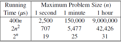
Table 4.4: Maximum size of a problem that can be solved in 1 second, 1 minute, and 1 hour, for various running times measured in microseconds.
The importance of good algorithm design goes beyond just what can be solved effectively on a given computer, however. As shown in Table 4.5, even if we achieve a dramatic speedup in hardware, we still cannot overcome the handicap of an asymptotically slow algorithm. This table shows the new maximum problem size achievable for any fixed amount of time, assuming algorithms with the given running times are now run on a computer 256 times faster than the previous one.
| Running Time | New Maximum Problem Size |
| 400n | 256m |
| 2n2 | 16m |
| 2n | m + 8 |
Table 4.5: Increase in the maximum size of a problem that can be solved in a fixed amount of time, by using a computer that is 256 times faster than the previous one. Each entry is a function of m, the previous maximum problem size.
Some Words of Caution
A few words of caution about asymptotic notation are in order at this point. First, note that the use of the big-Oh and related notations can be somewhat misleading should the constant factors they “hide” be very large. For example, while it is true that the function 10100n is O(n), if this is the running time of an algorithm being compared to one whose running time is 10n log n, we should prefer the O(nlog n)-time algorithm, even though the linear-time algorithm is asymptotically faster. This preference is because the constant factor, 10100, which is called “one googol,” is believed by many astronomers to be an upper bound on the number of atoms in the observable universe. So we are unlikely to ever have a real-world problem that has this number as its input size.
The observation above raises the issue of what constitutes a “fast” algorithm. Generally speaking, any algorithm running in O(n log n) time (with a reasonable constant factor) should be considered efficient. Even an O(n2)-time function may be fast enough in some contexts, that is, when n is small. But an algorithm whose running time is an exponential function, e.g., O(2n), should almost never be considered efficient.
Exponential Running Times
To see how fast the function 2n grows, consider the famous story about the inventor of the game of chess. He asked only that his king pay him 1 grain of rice for the first square on the board, 2 grains for the second, 4 grains for the third, 8 for the fourth, and so on. The number of grains in the 64th square would be
263 = 9, 223, 372, 036, 854, 775, 808,
which is about nine billion billions!
If we must draw a line between efficient and inefficient algorithms, therefore, it is natural to make this distinction be that between those algorithms running in polynomial time and those running in exponential time. That is, make the distinction between algorithms with a running time that is O(nc), for some constant c > 1, and those with a running time that is O(bn), for some constant b > 1. Like so many notions we have discussed in this section, this too should be taken with a “grain of salt,” for an algorithm running in O(n100) time should probably not be considered “efficient.” Even so, the distinction between polynomial-time and exponential-time algorithms is considered a robust measure of tractability.
4.3.3 Examples of Algorithm Analysis
Now that we have the big-Oh notation for doing algorithm analysis, let us give some examples by characterizing the running time of some simple algorithms using this notation. Moreover, in keeping with our earlier promise, we will illustrate below how each of the seven functions given earlier in this chapter can be used to characterize the running time of an example algorithm.
Constant-Time Operations
All of the primitive operations, originally described on page 154, are assumed to run in constant time; formally, we say they run in O(1) time. We wish to emphasize several important constant-time operations that involve arrays. Assume that variable A is an array of n elements. The expression A.length in Java is evaluated in constant time, because arrays are represented internally with an explicit variable that records the length of the array. Another central behavior of arrays is that for any valid index j, the individual element, A[j], can be accessed in constant time. This is because an array uses a consecutive block of memory. The jth element can be found, not by iterating through the array one element at a time, but by validating the index, and using it as an offset from the beginning of the array in determining the appropriate memory address. Therefore, we say that the expression A[j] is evaluated in O(1) time for an array.
Finding the Maximum of an Array
As a classic example of an algorithm with a running time that grows proportional to n, we consider the goal of finding the largest element of an array. A typical strategy is to loop through elements of the array while maintaining as a variable the largest element seen thus far. Code Fragment 4.3 presents a method named arrayMax implementing this strategy.

Code Fragment 4.3: A method that returns the maximum value of an array.
Using the big-Oh notation, we can write the following mathematically precise statement on the running time of algorithm arrayMax for any computer.
Proposition 4.16: The algorithm, arrayMax, for computing the maximum element of an array of n numbers, runs in O(n) time.
Justification: The initialization at lines 3 and 4 and the return statement at line 8 require only a constant number of primitive operations. Each iteration of the loop also requires only a constant number of primitive operations, and the loop executes n − 1 times. Therefore, we account for the number of primitive operations being c′ · (n − 1) + c″ for appropriate constants c′ and c″ that reflect, respectively, the work performed inside and outside the loop body. Because each primitive operation runs in constant time, we have that the running time of algorithm arrayMax on an input of size n is at most c′ · (n − 1) + c″ = c′ · n + (c″ − c′) ≤ c′ · n if we assume, without loss of generality, that c″ ≤ c′. We conclude that the running time of algorithm arrayMax is 0(n).
Further Analysis of the Maximum-Finding Algorithm
A more interesting question about arrayMax is how many times we might update the current “biggest” value. In the worst case, if the data is given to us in increasing order, the biggest value is reassigned n − 1 times. But what if the input is given to us in random order, with all orders equally likely; what would be the expected number of times we update the biggest value in this case? To answer this question, note that we update the current biggest in an iteration of the loop only if the current element is bigger than all the elements that precede it. If the sequence is given to us in random order, the probability that the jth element is the largest of the first j elements is 1/j (assuming uniqueness). Hence, the expected number of times we update the biggest (including initialization) is ![]() , which is known as the nth Harmonic number. It can be shown that Hn is O(logn). Therefore, the expected number of times the biggest value is updated by arrayMax on a randomly ordered sequence is O(logn).
, which is known as the nth Harmonic number. It can be shown that Hn is O(logn). Therefore, the expected number of times the biggest value is updated by arrayMax on a randomly ordered sequence is O(logn).
Composing Long Strings
As our next example, we revisit the experimental study from Section 4.1, in which we examined two different implementations for composing a long string (see Code Fragment 4.2). Our first algorithm was based on repeated use of the string concatenation operator; for convenience, that method is also given in Code Fragment 4.4.

Code Fragment 4.4: Composing a string using repeated concatenation.
The most important aspect of this implementation is that strings in Java are immutable objects. Once created, an instance cannot be modified. The command, answer += c, is shorthand for answer = (answer + c). This command does not cause a new character to be added to the existing String instance; instead it produces a new String with the desired sequence of characters, and then it reassigns the variable, answer, to refer to that new string.
In terms of efficiency, the problem with this interpretation is that the creation of a new string as a result of a concatenation, requires time that is proportional to the length of the resulting string. The first time through this loop, the result has length 1, the second time through the loop the result has length 2, and so on, until we reach the final string of length n. Therefore, the overall time taken by this algorithm is proportional to
1 + 2 + ··· + n,
which we recognize as the familiar O(n2) summation from Proposition 4.3. Therefore, the total time complexity of the repeat1 algorithm is O(n2).
We see this theoretical analysis reflected in the experimental results. The running time of a quadratic algorithm should theoretically quadruple if the size of the problem doubles, as (2n)2 = 4 · n2. (We say “theoretically,” because this does not account for lower-order terms that are hidden by the asymptotic notation.) We see such an approximate fourfold increase in the running time of repeat1 in Table 4.1 on page 152.
In contrast, the running times in that table for the repeat2 algorithm, which uses Java's StringBuilder class, demonstrate a trend of approximately doubling each time the problem size doubles. The StringBuilder class relies on an advanced technique with a worst-case running time of O(n) for composing a string of length n; we will later explore that technique as the focus of Section 7.2.1.
Three-Way Set Disjointness
Suppose we are given three sets, A, B, and C, stored in three different integer arrays. We will assume that no individual set contains duplicate values, but that there may be some numbers that are in two or three of the sets. The three-way set disjointness problem is to determine if the intersection of the three sets is empty, namely, that there is no element x such that x ∈ A, x ∈ B, and x ∈ C. A simple Java method to determine this property is given in Code Fragment 4.5.

Code Fragment 4.5: Algorithm disjoint1 for testing three-way set disjointness.
This simple algorithm loops through each possible triple of values from the three sets to see if those values are equivalent. If each of the original sets has size n, then the worst-case running time of this method is O(n3).
We can improve upon the asymptotic performance with a simple observation. Once inside the body of the loop over B, if selected elements a and b do not match each other, it is a waste of time to iterate through all values of C looking for a matching triple. An improved solution to this problem, taking advantage of this observation, is presented in Code Fragment 4.6.

Code Fragment 4.6: Algorithm disjoint2 for testing three-way set disjointness.
In the improved version, it is not simply that we save time if we get lucky. We claim that the worst-case running time for disjoint2 is O(n2). There are quadratically many pairs (a,b) to consider. However, if A and B are each sets of distinct elements, there can be at most O(n) such pairs with a equal to b. Therefore, the innermost loop, over C, executes at most n times.
To account for the overall running time, we examine the time spent executing each line of code. The management of the for loop over A requires O(n) time. The management of the for loop over B accounts for a total of O(n2) time, since that loop is executed n different times. The test a == b is evaluated O(n2) times. The rest of the time spent depends upon how many matching (a,b) pairs exist. As we have noted, there are at most n such pairs; therefore, the management of the loop over C and the commands within the body of that loop use at most O(n2) time. By our standard application of Proposition 4.8, the total time spent is O(n2).
Element Uniqueness
A problem that is closely related to the three-way set disjointness problem is the element uniqueness problem. In the former, we are given three sets and we presumed that there were no duplicates within a single set. In the element uniqueness problem, we are given an array with n elements and asked whether all elements of that collection are distinct from each other.
Our first solution to this problem uses a straightforward iterative algorithm. The uniquel method, given in Code Fragment 4.7, solves the element uniqueness problem by looping through all distinct pairs of indices j < k, checking if any of those pairs refer to elements that are equivalent to each other. It does this using two nested for loops, such that the first iteration of the outer loop causes n − 1 iterations of the inner loop, the second iteration of the outer loop causes n − 2 iterations of the inner loop, and so on. Thus, the worst-case running time of this method is proportional to
(n − 1) + (n − 2) + ··· + 2 + 1,
which we recognize as the familiar O(n2) summation from Proposition 4.3.

Code Fragment 4.7: Algorithm unique1 for testing element uniqueness.
Using Sorting as a Problem-Solving Tool
An even better algorithm for the element uniqueness problem is based on using sorting as a problem-solving tool. In this case, by sorting the array of elements, we are guaranteed that any duplicate elements will be placed next to each other. Thus, to determine if there are any duplicates, all we need to do is perform a single pass over the sorted array, looking for consecutive duplicates.
A Java implementation of this algorithm is given in Code Fragment 4.8. (See Section 3.1.3 for discussion of the java.util.Arrays class.)

Code Fragment 4.8: Algorithm unique2 for testing element uniqueness.
Sorting algorithms will be the focus of Chapter 12. The best sorting algorithms (including those used by Array.sort in Java) guarantee a worst-case running time of O(nlog n). Once the data is sorted, the subsequent loop runs in O(n) time, and so the entire unique2 algorithm runs in O(n log n) time. Exercise C-4.35 explores the use of sorting to solve the three-way set disjointness problem in O(n log n) time.
Prefix Averages
The next problem we consider is computing what are known as prefix averages of a sequence of numbers. Namely, given a sequence x consisting of n numbers, we want to compute a sequence a such that aj is the average of elements x0, ..., xj, for j = 0, ..., n − 1, that is,
![]()
Prefix averages have many applications in economics and statistics. For example, given the year-by-year returns of a mutual fund, ordered from recent to past, an investor will typically want to see the fund's average annual returns for the most recent year, the most recent three years, the most recent five years, and so on. Likewise, given a stream of daily Web usage logs, a website manager may wish to track average usage trends over various time periods. We present two implementation for computing prefix averages, yet with significantly different running times.
A Quadratic-Time Algorithm
Our first algorithm for computing prefix averages, denoted as prefixAverage1, is shown in Code Fragment 4.9. It computes each element aj independently, using an inner loop to compute that partial sum.
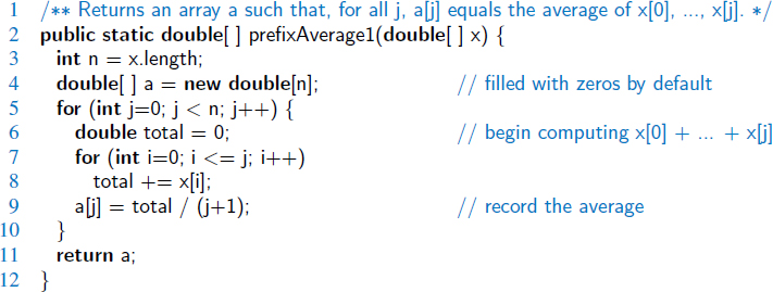
Code Fragment 4.9: Algorithm prefixAverage1.
Let us analyze the prefixAverage1 algorithm.
- The initialization of n = x.length at line 3 and the eventual return of a reference to array a at line 11 both execute in O(1) time.
- Creating and initializing the new array, a, at line 4 can be done with in O(n) time, using a constant number of primitive operations per element.
- There are two nested for loops, which are controlled, respectively, by counters j and i. The body of the outer loop, controlled by counter j, is executed n times, for j = 0, ..., n − 1. Therefore, statements total = 0 and a[j] = total / (j+1) are executed n times each. This implies that these two statements, plus the management of counter j in the loop, contribute a number of primitive operations proportional to n, that is, O(n) time.
- The body of the inner loop, which is controlled by counter i, is executed j + 1 times, depending on the current value of the outer loop counter j. Thus, statement total += x[i], in the inner loop, is executed 1 + 2 + 3 + ··· + n times. By recalling Proposition 4.3, we know that 1 + 2 + 3 + ··· + n = n(n + 1)/2, which implies that the statement in the inner loop contributes O(n2) time. A similar argument can be done for the primitive operations associated with maintaining counter i, which also take O(n2) time.
The running time of implementation prefixAverage1 is given by the sum of these terms. The first term is O(1), the second and third terms are O(n), and the fourth term is O(n2). By a simple application of Proposition 4.8, the running time of prefixAverage1 is O(n2).
A Linear-Time Algorithm
An intermediate value in the computation of the prefix average is the prefix sum x0 + x1 + ··· + xj, denoted as total in our first implementation; this allows us to compute the prefix average a[j] = total / (j + 1). In our first algorithm, the prefix sum is computed anew for each value of j. That contributed O(j) time for each j, leading to the quadratic behavior.
For greater efficiency, we can maintain the current prefix sum dynamically, effectively computing x0 + x1 + ··· + xj as total + xj, where value total is equal to the sum x0 + x1 + ··· + xj − 1, when computed by the previous pass of the loop over j. Code Fragment 4.10 provides a new implementation, denoted as prefixAverage2, using this approach.

Code Fragment 4.10: Algorithm prefixAverage2.
The analysis of the running time of algorithm prefixAverage2 follows:
- Initializing variables n and total uses O(1) time.
- Initializing the array a uses O(n) time.
- There is a single for loop, which is controlled by counter j. The maintenance of that loop contributes a total of O(n) time.
- The body of the loop is executed n times, for j = 0, ..., n − 1. Thus, statements total += x[j] and a[j] = total / (j+1) are executed n times each. Since each of these statements uses O(1) time per iteration, their overall contribution is O(n) time.
- The eventual return of a reference to array A uses O(1) time.
The running time of algorithm prefixAverage2 is given by the sum of the five terms. The first and last are O(1) and the remaining three are O(n). By a simple application of Proposition 4.8, the running time of prefixAverage2 is O(n), which is much better than the quadratic time of algorithm prefixAverage1.
4.4 Simple Justification Techniques
Sometimes, we will want to make claims about an algorithm, such as showing that it is correct or that it runs fast. In order to rigorously make such claims, we must use mathematical language, and in order to back up such claims, we must justify or prove our statements. Fortunately, there are several simple ways to do this.
4.4.1 By Example
Some claims are of the generic form, “There is an element x in a set S that has property P.” To justify such a claim, we only need to produce a particular x in S that has property P. Likewise, some hard-to-believe claims are of the generic form, “Every element x in a set S has property P.” To justify that such a claim is false, we only need to produce a particular x from S that does not have property P. Such an instance is called a counterexample.
Example 4.17: Professor Amongus claims that every number of the form 2i − 1 is a prime, when i is an integer greater than 1. Professor Amongus is wrong.
Justification: To prove Professor Amongus is wrong, we find a counterexample. Fortunately, we need not look too far, for 24 − 1 = 15 = 3 · 5.
4.4.2 The “Contra” Attack
Another set of justification techniques involves the use of the negative. The two primary such methods are the use of the contrapositive and the contradiction. To justify the statement “if p is true, then q is true,” we establish that “if q is not true, then p is not true” instead. Logically, these two statements are the same, but the latter, which is called the contrapositive of the first, may be easier to think about.
Example 4.18: Let a and b be integers. If ab is even, then a is even or b is even.
Justification: To justify this claim, consider the contrapositive, “If a is odd and b is odd, then ab is odd.” So, suppose a = 2j + 1 and b = 2k + 1, for some integers j and k. Then ab = 4jk + 2j + 2k + 1 = 2(2jk + j + k) + 1; hence, ab is odd.
Besides showing a use of the contrapositive justification technique, the previous example also contains an application of de Morgan's law. This law helps us deal with negations, for it states that the negation of a statement of the form “p or q” is “not p and not q.” Likewise, it states that the negation of a statement of the form “p and q” is “not p or not q.”
Contradiction
Another negative justification technique is justification by contradiction, which also often involves using de Morgan's law. In applying the justification by contradiction technique, we establish that a statement q is true by first supposing that q is false and then showing that this assumption leads to a contradiction (such as 2 ≠ 2 or 1 > 3). By reaching such a contradiction, we show that no consistent situation exists with q being false, so q must be true. Of course, in order to reach this conclusion, we must be sure our situation is consistent before we assume q is false.
Example 4.19: Let a and b be integers. If ab is odd, then a is odd and b is odd.
Justification: Let ab be odd. We wish to show that a is odd and b is odd. So, with the hope of leading to a contradiction, let us assume the opposite, namely, suppose a is even or b is even. In fact, without loss of generality, we can assume that a is even (since the case for b is symmetric). Then a = 2j for some integer j. Hence, ab = (2j)b = 2(jb), that is, ab is even. But this is a contradiction: ab cannot simultaneously be odd and even. Therefore, a is odd and b is odd.
4.4.3 Induction and Loop Invariants
Most of the claims we make about a running time or a space bound involve an integer parameter n (usually denoting an intuitive notion of the “size” of the problem). Moreover, most of these claims are equivalent to saying some statement q(n) is true “for all n ≥ 1.” Since this is making a claim about an infinite set of numbers, we cannot justify this exhaustively in a direct fashion.
Induction
We can often justify claims such as those above as true, however, by using the technique of induction. This technique amounts to showing that, for any particular n ≥ 1, there is a finite sequence of implications that starts with something known to be true and ultimately leads to showing that q(n) is true. Specifically, we begin a justification by induction by showing that q(n) is true for n = 1 (and possibly some other values n = 2,3, ..., k, for some constant k). Then we justify that the inductive “step” is true for n > k, namely, we show “if q(j) is true for all j < n, then q(n) is true.” The combination of these two pieces completes the justification by induction.
Proposition 4.20: Consider the Fibonacci function F(n), which is defined such that F(1) = 1, F(2) = 2, and F(n) = F(n − 2) + F(n − 1) for n > 2. (See Section 2.2.3.) We claim that F(n) < 2n.
Justification: We will show our claim is correct by induction.
Base cases: (n ≤ 2). F(1) = 1 < 2 = 21 and F(2) = 2 < 4 = 22.
Induction step: (n > 2). Suppose our claim is true for all j < n. Since both n − 2 and n − 1 are less than n, we can apply the inductive assumption (sometimes called the “inductive hypothesis”) to imply that
F(n) = F(n−2) + F(n−1) < 2n−2 + 2n−1.
Since
2n−2 + 2n−1 < 2n−1 + 2n−1 = 2 · 2n−1 = 2n,
we have that F(n) < 2n, thus showing the inductive hypothesis for n.
Let us do another inductive argument, this time for a fact we have seen before.
Proposition 4.21: (which is the same as Proposition 4.3)

Justification: We will justify this equality by induction.
Base case: n = 1. Trivial, for 1 = n(n + 1)/2, if n = 1.
Induction step: n ≥ 2. Assume the inductive hypothesis is true for any j < n. Therefore, for j = n − 1, we have

Hence, we obtain

thereby proving the inductive hypothesis for n.
We may sometimes feel overwhelmed by the task of justifying something true for all n ≥ 1. We should remember, however, the concreteness of the inductive technique. It shows that, for any particular n, there is a finite step-by-step sequence of implications that starts with something true and leads to the truth about n. In short, the inductive argument is a template for building a sequence of direct justifications.
Loop Invariants
The final justification technique we discuss in this section is the loop invariant. To prove some statement ![]() about a loop is correct, define
about a loop is correct, define ![]() in terms of a series of smaller statements
in terms of a series of smaller statements ![]() 0,
0, ![]() 1,...,
1,..., ![]() k, where:
k, where:
- The initial claim,
 0, is true before the loop begins.
 - If j−1 is true before iteration j, then j will be true after iteration j.
- The final statement, k, implies the desired statement L to be true.
Let us give a simple example of using a loop-invariant argument to justify the correctness of an algorithm. In particular, we use a loop invariant to justify that the method arrayFind (see Code Fragment 4.11) finds the smallest index at which element val occurs in array A.

Code Fragment 4.11: Algorithm arrayFind for finding the first index at which a given element occurs in an array.
To show that arrayFind is correct, we inductively define a series of statements, ![]() j, that lead to the correctness of our algorithm. Specifically, we claim the following is true at the beginning of iteration j of the while loop:
j, that lead to the correctness of our algorithm. Specifically, we claim the following is true at the beginning of iteration j of the while loop:
![]() j: val is not equal to any of the first j elements of data.
j: val is not equal to any of the first j elements of data.
This claim is true at the beginning of the first iteration of the loop, because j is 0 and there are no elements among the first 0 in data (this kind of a trivially true claim is said to hold vacuously). In iteration j, we compare element val to element data [j]; if these two elements are equivalent, we return the index j, which is clearly correct since no earlier elements equal val. If the two elements val and data[j] are not equal, then we have found one more element not equal to val and we increment the index j. Thus, the claim ![]() j will be true for this new value of j; hence, it is true at the beginning of the next iteration. If the while loop terminates without ever returning an index in data, then we have j = n. That is,
j will be true for this new value of j; hence, it is true at the beginning of the next iteration. If the while loop terminates without ever returning an index in data, then we have j = n. That is, ![]() n is true—there are no elements of data equal to val. Therefore, the algorithm correctly returns −1 to indicate that val is not in data.
n is true—there are no elements of data equal to val. Therefore, the algorithm correctly returns −1 to indicate that val is not in data.
4.5 Exercises
Reinforcement
| R-4.1 | Graph the functions 8n, 4n log n, 2n2, n3, and 2n using a logarithmic scale for the x- and y-axes; that is, if the function value f(n) is y, plot this as a point with x-coordinate at logn and y-coordinate at log y. |
| R-4.2 | The number of operations executed by algorithms A and B is 8nlogn and 2n2, respectively. Determine n0 such that A is better than B for n ≥ n0. |
| R-4.3 | The number of operations executed by algorithms A and B is 40n2 and 2n3, respectively. Determine n0 such that A is better than B for n ≥ n0. |
| R-4.4 | Give an example of a function that is plotted the same on a log-log scale as it is on a standard scale. |
| R-4.5 | Explain why the plot of the function nc is a straight line with slope c on a log-log scale. |
| R-4.6 | What is the sum of all the even numbers from 0 to 2n, for any integer n ≥ 1? |
| R-4.7 | Show that the following two statements are equivalent:
|
| R-4.8 | Order the following functions by asymptotic growth rate.
|
| R-4.9 | Give a big-Oh characterization, in terms of n, of the running time of the example1 method shown in Code Fragment 4.12. |
| R-4.10 | Give a big-Oh characterization, in terms of n, of the running time of the example2 method shown in Code Fragment 4.12. |
| R-4.11 | Give a big-Oh characterization, in terms of n, of the running time of the example3 method shown in Code Fragment 4.12. |
| R-4.12 | Give a big-Oh characterization, in terms of n, of the running time of the example4 method shown in Code Fragment 4.12. |
| R-4.13 | Give a big-Oh characterization, in terms of n, of the running time of the example5 method shown in Code Fragment 4.12. |
| R-4.14 | Show that if d(n) is O(f(n)), then ad(n) is O(f(n)), for any constant a > 0. |
| R-4.15 | Show that if d(n) is O(f(n)) and e(n) is O(g(n)), then the product d(n)e(n) is O(f(n)g(n)). |
| R-4.16 | Show that if d(n) is O(f(n)) and e(n) is O(g(n)), then d(n) + e(n) is O(f(n) + g(n)).
Code Fragment 4.12: Some sample algorithms for analysis. |
| R-4.17 | Show that if d(n) is O(f(n)) and e(n) is O(g(n)), then d(n) − e(n) is not necessarily O(f(n) − g(n)). |
| R-4.18 | Show that if d(n) is O(f(n)) and f(n) is O(g(n)), then d(n) is O(g(n)). |
| R-4.19 | Show that O(max{f(n),g(n)}) = O(f(n)+ g(n)). |
| R-4.20 | Show that f(n) is O(g(n)) if and only if g(n) is Ω(f(n)). |
| R-4.21 | Show that if p(n) is a polynomial in n, then logp(n) is O(logn). |
| R-4.22 | Show that (n + 1)5 is O(n5). |
| R-4.23 | Show that 2n+1 is O(2n). |
| R-4.24 | Show that n is O(n log n). |
| R-4.25 | Show that n2 is Ω(n log n). |
| R-4.26 | Show that n logn is Ω(n). |
| R-4.27 | Show that |
| R-4.28 | For each function f(n) and time t in the following table, determine the largest size n of a problem P that can be solved in time t if the algorithm for solving P takes f(n) microseconds (one entry is already completed).
|
| R-4.29 | Algorithm A executes an O(logn)-time computation for each entry of an array storing n elements. What is its worst-case running time? |
| R-4.30 | Given an n-element array X, Algorithm B chooses logn elements in X at random and executes an O(n)-time calculation for each. What is the worst-case running time of Algorithm B? |
| R-4.31 | Given an n-element array X of integers, Algorithm C executes an O(n)-time computation for each even number in X, and an O(logn)-time computation for each odd number in X. What are the best-case and worst-case running times of Algorithm C? |
| R-4.32 | Given an n-element array X, Algorithm D calls Algorithm E on each element X[i]. Algorithm E runs in O(i) time when it is called on element X[i]. What is the worst-case running time of Algorithm D? |
| R-4.33 | Al and Bob are arguing about their algorithms. Al claims his O(n log n)-time method is always faster than Bob's O(n2)-time method. To settle the issue, they perform a set of experiments. To Al's dismay, they find that if n < 100, the O(n2)-time algorithm runs faster, and only when n ≥ 100 is the O(n log n)-time one better. Explain how this is possible. |
| R-4.34 | There is a well-known city (which will go nameless here) whose inhabitants have the reputation of enjoying a meal only if that meal is the best they have ever experienced in their life. Otherwise, they hate it. Assuming meal quality is distributed uniformly across a person's life, describe the expected number of times inhabitants of this city are happy with their meals? |


Creativity
| C-4.35 | Assuming it is possible to sort n numbers in O(n log n) time, show that it is possible to solve the three-way set disjointness problem in O(n log n) time. |
| C-4.36 | Describe an efficient algorithm for finding the ten largest elements in an array of size n. What is the running time of your algorithm? |
| C-4.37 | Give an example of a positive function f(n) such that f(n) is neither O(n) nor Ω(n). |
| C-4.38 | Show that |
| C-4.39 | Show that |
| C-4.40 | Determine the total number of grains of rice requested by the inventor of chess. |
| C-4.41 | Show that logbf(n) is Θ(logf(n)) if b > 1 is a constant. |
| C-4.42 | Describe an algorithm for finding both the minimum and maximum of n numbers using fewer than 3n/2 comparisons. |
| C-4.43 | Bob built a website and gave the URL only to his n friends, which he numbered from 1 to n. He told friend number i that he/she can visit the website at most i times. Now Bob has a counter, C, keeping track of the total number of visits to the site (but not the identities of who visits). What is the minimum value for C such that Bob can know that one of his friends has visited his/her maximum allowed number of times? |
| C-4.44 | Draw a visual justification of Proposition 4.3 analogous to that of Figure 4.3(b) for the case when n is odd. |
| C-4.45 | An array A contains n − 1 unique integers in the range [0, n − 1], that is, there is one number from this range that is not in A . Design an O(n)-time algorithm for finding that number. You are only allowed to use O(1) additional space besides the array A itself. |
| C-4.46 | Perform an asymptotic analysis of the insertion-sort algorithm given in Section 3.1.2. What are the worst-case and best-case running times? |
| C-4.47 | Communication security is extremely important in computer networks, and one way many network protocols achieve security is to encrypt messages. Typical cryptographic schemes for the secure transmission of messages over such networks are based on the fact that no efficient algorithms are known for factoring large integers. Hence, if we can represent a secret message by a large prime number p, we can transmit, over the network, the number r = p · q, where q > p is another large prime number that acts as the encryption key. An eavesdropper who obtains the transmitted number r on the network would have to factor r in order to figure out the secret message p.
Using factoring to figure out a message is hard without knowing the encryption key q. To understand why, consider the following naive factoring algorithm: for (int p=2; p < r; p++) if (r % p == 0) return "The secret message is p!";
|
| C-4.48 | Al says he can prove that all sheep in a flock are the same color:
Base case: One sheep. It is clearly the same color as itself. Induction step: A flock of n sheep. Take a sheep, a, out. The remaining n − 1 are all the same color by induction. Now put sheep a back in and take out a different sheep, b. By induction, the n − 1 sheep (now with a) are all the same color. Therefore, all the sheep in the flock are the same color. What is wrong with Al's “justification”? |
| C-4.49 | Consider the following “justification” that the Fibonacci function, F(n) is O(n):
Base case (n ≤ 2): F(1) = 1 and F(2) = 2. Induction step (n > 2): Assume claim true for n′ < n. Consider n. F(n) = F(n − 2) + F(n − 1). By induction, F(n − 2) is O(n − 2) and F(n − 1) is O(n − 1). Then, F(n) is O((n − 2) + (n − 1)), by the identity presented in Exercise R-4.16. Therefore, F(n) is O(n). What is wrong with this “justification”? |
| C-4.50 | Consider the Fibonacci function, F(n) (see Proposition 4.20). Show by induction that F(n) is Ω((3/2)n). |
| C-4.51 | Let S be a set of n lines in the plane such that no two are parallel and no three meet in the same point. Show, by induction, that the lines in S determine Θ(n2) intersection points. |
| C-4.52 | Show that the summation |
| C-4.53 | Show that the summation |
| C-4.54 | Let p(x) be a polynomial of degree n, that is,
p(x) = a0 + x(a1 + x(a2 + x(a3 + ··· + x(an−1 + xan) ···))), which is known as Horner's method. Using the big-Oh notation, characterize the number of arithmetic operations this method executes. |
| C-4.55 | An evil king has n bottles of wine, and a spy has just poisoned one of them. Unfortunately, they do not know which one it is. The poison is very deadly; just one drop diluted even a billion to one will still kill. Even so, it takes a full month for the poison to take effect. Design a scheme for determining exactly which one of the wine bottles was poisoned in just one month's time while expending O(logn) taste testers. |
| C-4.56 | An array A contains n integers taken from the interval [0,4n], with repetitions allowed. Describe an efficient algorithm for determining an integer value k that occurs the most often in A. What is the running time of your algorithm? |
| C-4.57 | Given an array A of n positive integers, each represented with |
| C-4.58 | Argue why any solution to the previous problem must run in Ω(n) time. |
| C-4.59 | Given an array A of n arbitrary integers, design an O(n)-time method for finding an integer that cannot be formed as the sum of two integers in A. |
Projects
| P-4.60 | Perform an experimental analysis of the two algorithms prefixAverage1 and prefixAverage2, from Section 4.3.3. Visualize their running times as a function of the input size with a log-log chart. |
| P-4.61 | Perform an experimental analysis that compares the relative running times of the methods shown in Code Fragment 4.12. |
| P-4.62 | Perform an experimental analysis to test the hypothesis that Java's Array.sort method runs in O(n log n) time on average. |
| P-4.63 | For each of the algorithms unique1 and unique2, which solve the element uniqueness problem, perform an experimental analysis to determine the largest value of n such that the given algorithm runs in one minute or less. |
Chapter Notes
The big-Oh notation has prompted several comments about its proper use [18, 43, 59]. Knuth [60, 59] defines it using the notation f(n) = O(g(n)), but says this “equality” is only “one way.” We have chosen to take a more standard view of equality and view the big-Oh notation as a set, following Brassard [18]. The reader interested in studying average-case analysis is referred to the book chapter by Vitter and Flajolet [93].