Chapter
11

Search Trees

Contents

11.1 Binary Search Trees

In Chapter 8 we introduced the tree data structure and demonstrated a variety of applications. One important use is as a search tree (as described on page 338). In this chapter, we use a search-tree structure to efficiently implement a sorted map. The three most fundamental methods of of a map (see Section 10.1.1) are:

get(k):	Returns the value v associated with key k, if such an entry exists; otherwise returns null.
put(k, v):	Associates value v with key k, replacing and returning any existing value if the map already contains an entry with key equal to k.
remove(k):	Removes the entry with key equal to k, if one exists, and returns its value; otherwise returns null.

The sorted map ADT includes additional functionality (see Section 10.3), guaranteeing that an iteration reports keys in sorted order, and supporting additional searches such as higherEntry(k) and subMap(k₁, k₂).

Binary trees are an excellent data structure for storing entries of a map, assuming we have an order relation defined on the keys. In this chapter, we define a binary search tree as a proper binary tree (see Section 8.2) such that each internal position p stores a key-value pair (k, v) such that:

• Keys stored in the left subtree of p are less than k.
• Keys stored in the right subtree of p are greater than k.

An example of such a binary search tree is given in Figure 11.1. Notice that the leaves of the tree serve only as “placeholders.” Their use as sentinels simplifies the presentation of several of our search and update algorithms. With care, they can be represented as null references in practice, thereby reducing the number of nodes in half (since there are more leaves than internal nodes in a proper binary tree).

Figure 11.1: A binary search tree with integer keys. We omit the display of associated values in this chapter, since they are not relevant to the order of entries within a search tree.

11.1.1 Searching Within a Binary Search Tree

The most important consequence of the structural property of a binary search tree is its namesake search algorithm. We can attempt to locate a particular key in a binary search tree by viewing it as a decision tree (recall Figure 8.5). In this case, the question asked at each internal position p is whether the desired key k is less than, equal to, or greater than the key stored at position p, which we denote as key(p). If the answer is “less than,” then the search continues in the left subtree. If the answer is “equal,” then the search terminates successfully. If the answer is “greater than,” then the search continues in the right subtree. Finally, if we reach a leaf, then the search terminates unsuccessfully. (See Figure 11.2.)

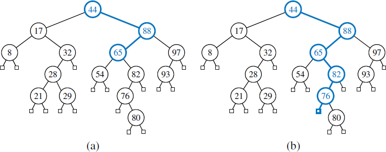
Figure 11.2: (a) A successful search for key 65 in a binary search tree; (b) an unsuccessful search for key 68 that terminates at the leaf to the left of the key 76.

We describe this approach in Code Fragment 11.1. If key k occurs in a subtree rooted at p, a call to TreeSearch(p, k) results in the position at which the key is found. For an unsuccessful search, the TreeSearch algorithm returns the final leaf explored on the search path (which we will later make use of when determining where to insert a new entry in a search tree).

Code Fragment 11.1: Recursive search in a binary search tree.

Analysis of Binary Tree Searching

The analysis of the worst-case running time of searching in a binary search tree T is simple. Algorithm TreeSearch is recursive and executes a constant number of primitive operations for each recursive call. Each recursive call of TreeSearch is made on a child of the previous position. That is, TreeSearch is called on the positions of a path of T that starts at the root and goes down one level at a time. Thus, the number of such positions is bounded by h + 1, where h is the height of T. In other words, since we spend O(1) time per position encountered in the search, the overall search runs in O(h) time, where h is the height of the binary search tree T. (See Figure 11.3.)

Figure 11.3: Illustrating the running time of searching in a binary search tree. The figure uses a standard visualization shortcut of a binary search tree as a big triangle and a path from the root as a zig-zag line.

In the context of the sorted map ADT, the search will be used as a subroutine for implementing the get method, as well as for the put and remove methods, since each of these begins by trying to locate an existing entry with the given key. We will later demonstrate how to implement sorted map operations, such as lowerEntry and higherEntry, by navigating within the tree after performing a standard search. All of these operations will run in worst-case O(h) time for a tree with height h.

Admittedly, the height h of T can be as large as the number of entries, n, but we expect that it is usually much smaller. Later in this chapter we will show various strategies to maintain an upper bound of O(logn) on the height of a search tree T.

11.1.2 Insertions and Deletions

Binary search trees allow implementations of the put and remove operations using algorithms that are fairly straightforward, although not trivial.

Insertion

The map operation put(k, v) begins with a search for an entry with key k. If found, that entry's existing value is reassigned. Otherwise, the new entry can be inserted into the underlying tree by expanding the leaf that was reached at the end of the failed search into an internal node. The binary search-tree property is sustained by that placement (note that it is placed exactly where a search would expect it). Let us assume a proper binary tree supports the following update operation:

expandExternal(p, e):

Stores entry e at the external position p, and expands p to be internal, having two new leaves as children.

We can then describe the TreeInsert algorithm with the pseudocode given in in Code Fragment 11.2. An example of insertion into a binary search tree is shown in Figure 11.4.

Code Fragment 11.2: Algorithm for inserting a key-value pair into a map that is represented as a binary search tree.

Figure 11.4: Insertion of an entry with key 68 into the search tree of Figure 11.2. Finding the position to insert is shown in (a), and the resulting tree is shown in (b).

Deletion

Deleting an entry from a binary search tree is a bit more complex than inserting a new entry because the position of an entry to be deleted might be anywhere in the tree (as opposed to insertions, which always occur at a leaf). To delete an entry with key k, we begin by calling TreeSearch(root(), k) to find the position p storing an entry with key equal to k (if any). If the search returns an external node, then there is no entry to remove. Otherwise, we distinguish between two cases (of increasing difficulty):

• If at most one of the children of position p is internal, the deletion of the entry at position p is easily implemented (see Figure 11.5). Let position r be a child of p that is internal (or an arbitrary child, if both are leaves). We will remove p and the leaf that is r's sibling, while promoting r upward to take the place of p. We note that all remaining ancestor-descendant relationships that remain in the tree after the operation existed before the operation; therefore, the binary search-tree property is maintained.
• If position p has two children, we cannot simply remove the node from the tree since this would create a “hole” and two orphaned children. Instead, we proceed as follows (see Figure 11.6):
  • We locate position r containing the entry having the greatest key that is strictly less than that of position p (its so-called predecessor in the ordering of keys). That predecessor will always be located in the rightmost internal position of the left subtree of position p.
  • We use r's entry as a replacement for the one being deleted at position p. Because r has the immediately preceding key in the map, any entries in p's right subtree will have keys greater than r and any other entries in p's left subtree will have keys less than r. Therefore, the binary search-tree property is satisfied after the replacement.
  • Having used r's entry as a replacement for p, we instead delete the node at position r from the tree. Fortunately, since r was located as the rightmost internal position in a subtree, r does not have an internal right child. Therefore, its deletion can be performed using the first (and simpler) approach.

As with searching and insertion, this algorithm for a deletion involves the traversal of a single path downward from the root, possibly moving an entry between two positions of this path, and removing a node from that path and promoting its child. Therefore, it executes in time O(h) where h is the height of the tree.

Figure 11.5: Deletion from the binary search tree of Figure 11.4b, where the entry to delete (with key 32) is stored at a position p with one child r : (a) before the deletion; (b) after the deletion.

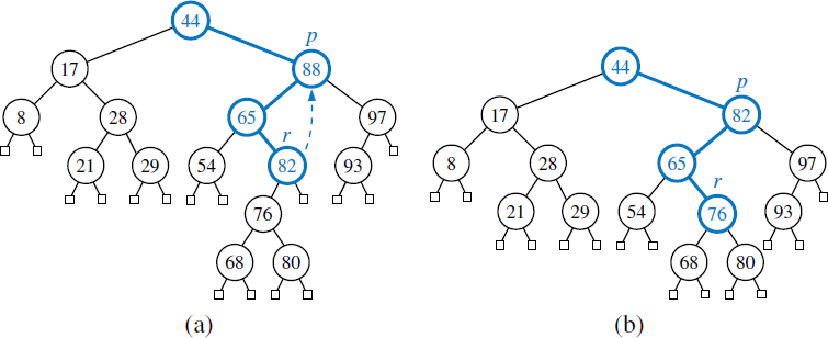
Figure 11.6: Deletion from the binary search tree of Figure 11.5b, where the entry to delete (with key 88) is stored at a position p with two children, and replaced by its predecessor r: (a) before the deletion; (b) after the deletion.

11.1.3 Java Implementation

In Code Fragments 11.3 through 11.6 we define a TreeMap class that implements the sorted map ADT while using a binary search tree for storage. The TreeMap class is declared as a child of the AbstractSortedMap base class, thereby inheriting support for performing comparisons based upon a given (or default) Comparator, a nested MapEntry class for storing key-value pairs, and concrete implementations of methods keySet and values based upon the entrySet method, which we will provide. (See Figure 10.2 on page 406 for an overview of our entire map hierarchy.)

For representing the tree structure, our TreeMap class maintains an instance of a subclass of the LinkedBinaryTree class from Section 8.3.1. In this implementation, we choose to represent the search tree as a proper binary tree, with explicit leaf nodes in the binary tree as sentinels, and map entries stored only at internal nodes. (We leave the task of a more space-efficient implementation to Exercise P-11.55.)

The TreeSearch algorithm of Code Fragment 11.1 is implemented as a private recursive method, treeSearch(p, k). That method either returns a position with an entry equal to key k, or else the last position that is visited on the search path. The method is not only used for all of the primary map operations, get(k), put(k, v), and remove(k), but for most of the sorted map methods, as the final internal position visited during an unsuccessful search has either the greatest key less than k or the least key greater than k.

Finally, we note that our TreeMap class is designed so that it can be subclassed to implement various forms of balanced search trees. We discuss the balancing framework more thoroughly in Section 11.2, but there are two aspects of the design that impact the code presented in this section. First, our tree member is technically declared as an instance of a BalanceableBinaryTree class, which is a specialization of the LinkedBinaryTree class; however, we rely only on the inherited behaviors in this section. Second, our code is peppered with calls to presumed methods named rebalanceAccess, rebalanceInsert, and rebalanceDelete; these methods do not do anything in this class, but they serve as hooks that can later be customized.

We conclude with a brief guide to the organization of our code.

Code Fragment 11.3:	Beginning of TreeMap class, including constructors, size method, and expandExternal and treeSearch utilities.
Code Fragment 11.4:	Map operations get(k), put(k, v), and remove(k).
Code Fragment 11.5:	Sorted map ADT methods lastEntry(), floorEntry(k), and lowerEntry(k), and protected utility treeMax. Symmetric methods firstEntry(), ceilingEntry(k), higherEntry(k), and treeMin are provided online.
Code Fragment 11.6:	Support for producing an iteration of all entries (method entrySet of the map ADT), or of a selected range of entries (method subMap(k1 k2) of the sorted map ADT).

Code Fragment 11.3: Beginning of a TreeMap class based on a binary search tree.

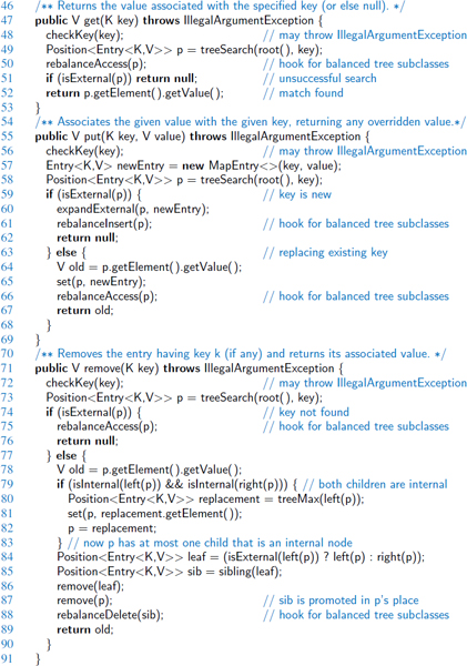
Code Fragment 11.4: Primary map operations for the TreeMap class.

Code Fragment 11.5: A sample of the sorted map operations for the TreeMap class. The symmetrical utility, treeMin, and public methods firstEntry, ceilingEntry, and higherEntry are available online.

Code Fragment 11.6: TreeMap operations supporting iteration of the entire map, or a portion of the map with a given key range.

11.1.4 Performance of a Binary Search Tree

An analysis of the operations of our TreeMap class is given in Table 11.1. Almost all operations have a worst-case running time that depends on h, where h is the height of the current tree. This is because most operations rely on traversing a path from the root of the tree, and the maximum path length within a tree is proportional to the height of the tree. Most notably, our implementations of map operations get, put, and remove, and most of the sorted map operations, each begins with a call to the treeSearch utility. Similar paths are traced when searching for the minimum or maximum entry in a subtree, a task used when finding a replacement during a deletion or in finding the overall first or last entry in the map. An iteration of the entire map is accomplished in O(n) time using an inorder traversal of the underlying tree, and the recursive subMap implementation can be shown to run in O(s + h) worst-case bound for a call that reports s results (see Exercise C-11.34).

Method	Running Time
size, isEmpty	O(1)
get, put, remove	O(h)
firstEntry, lastEntry	O(h)
ceilingEntry, floorEntry, lowerEntry, higherEntry	O(h)
subMap	O(s + h)
entrySet, keySet, values	O(n)

Table 11.1: Worst-case running times of the operations for a TreeMap. We denote the current height of the tree with h, and the number of entries reported by subMap as s. The space usage is O(n), where n is the number of entries stored in the map.

A binary search tree T is therefore an efficient implementation of a map with n entries only if its height is small. In the best case, T has height , which yields logarithmic-time performance for most of the map operations. In the worst case, however, T has height n, in which case it would look and feel like an ordered list implementation of a map. Such a worst-case configuration arises, for example, if we insert entries with keys in increasing or decreasing order. (See Figure 11.7.)

Figure 11.7: Example of a binary search tree with linear height, obtained by inserting entries in increasing order of their keys.

We can nevertheless take comfort that, on average, a binary search tree with n keys generated from a random series of insertions and removals of keys has expected height O(logn); the justification of this statement is beyond the scope of the book, requiring careful mathematical language to precisely define what we mean by a random series of insertions and removals, and sophisticated probability theory.

In applications where one cannot guarantee the random nature of updates, it is better to rely on variations of search trees, presented in the remainder of this chapter, that guarantee a worst-case height of O(logn), and thus O(logn) worst-case time for searches, insertions, and deletions.

11.2 Balanced Search Trees

In the closing of the previous section, we noted that if we could assume a random series of insertions and removals, the standard binary search tree supports O(logn) expected running times for the basic map operations. However, we may only claim O(n) worst-case time, because some sequences of operations may lead to an unbalanced tree with height proportional to n.

In the remainder of this chapter, we will explore four search-tree algorithms that provide stronger performance guarantees. Three of the four data structures (AVL trees, splay trees, and red-black trees) are based on augmenting a standard binary search tree with occasional operations to reshape the tree and reduce its height.

The primary operation to rebalance a binary search tree is known as a rotation. During a rotation, we “rotate” a child to be above its parent, as diagrammed in Figure 11.8.

Figure 11.8: A rotation operation in a binary search tree. A rotation can be per-formed to transform the left formation into the right, or the right formation into the left. Note that all keys in subtree T₁ have keys less than that of position x, all keys in subtree T₂ have keys that are between those of positions x and y, and all keys in subtree T₃ have keys that are greater than that of position y.

To maintain the binary search-tree property through a rotation, we note that if position x was a left child of position y prior to a rotation (and therefore the key of x is less than the key of y), then y becomes the right child of x after the rotation, and vice versa. Furthermore, we must relink the subtree of entries with keys that lie between the keys of the two positions that are being rotated. For example, in Figure 11.8 the subtree labeled T₂ represents entries with keys that are known to be greater than that of position x and less than that of position y. In the first configuration of that figure, T₂ is the right subtree of position x; in the second configuration, it is the left subtree of position y.

Because a single rotation modifies a constant number of parent-child relationships, it can be implemented in O(1) time with a linked binary tree representation.

In the context of a tree-balancing algorithm, a rotation allows the shape of a tree to be modified while maintaining the search-tree property. If used wisely, this operation can be performed to avoid highly unbalanced tree configurations. For example, a rightward rotation from the first formation of Figure 11.8 to the second reduces the depth of each node in subtree T₁ by one, while increasing the depth of each node in subtree T₃ by one. (Note that the depth of nodes in subtree T₂ are unaffected by the rotation.)

One or more rotations can be combined to provide broader rebalancing within a tree. One such compound operation we consider is a trinode restructuring. For this manipulation, we consider a position x, its parent y, and its grandparent z. The goal is to restructure the subtree rooted at z in order to reduce the overall path length to x and its subtrees. Pseudocode for a restructure(x) method is given in Code Fragment 11.7 and illustrated in Figure 11.9. In describing a trinode restructuring, we temporarily rename the positions x, y, and z as a, b, and c, so that a precedes b and b precedes c in an inorder traversal of T. There are four possible orientations mapping x, y, and z to a, b, and c, as shown in Figure 11.9, which are unified into one case by our relabeling. The trinode restructuring replaces z with the node identified as b, makes the children of this node be a and c, and makes the children of a and c be the four previous children of x, y, and z (other than x and y), while maintaining the inorder relationships of all the nodes in T.

Code Fragment 11.7: The trinode restructuring operation in a binary search tree.

In practice, the modification of a tree T caused by a trinode restructuring operation can be implemented through case analysis either as a single rotation (as in Figure 11.9a and b) or as a double rotation (as in Figure 11.9c and d). The double rotation arises when position x has the middle of the three relevant keys and is first rotated above its parent, and then above what was originally its grandparent. In any of the cases, the trinode restructuring is completed with O(1) running time.

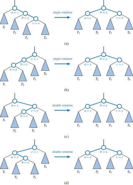
Figure 11.9: Schematic illustration of a trinode restructuring operation: (a and b) require a single rotation; (c and d) require a double rotation.

11.2.1 Java Framework for Balancing Search Trees

Our TreeMap class (introduced in Section 11.1.3) is a fully functional map implementation. However, the running time for its operations depend on the height of the tree, and in the worst-case, that height may be O(n) for a map with n entries. Therefore, we have intentionally designed the TreeMap class in a way that allows it to be easily extended to provide more advanced tree-balancing strategies. In later sections of this chapter, we will implement subclasses AVLTreeMap, SplayTreeMap, and RBTreeMap. In this section, we describe three important forms of support that the TreeMap class offers these subclasses.

Hooks for Rebalancing Operations

Our implementation of the basic map operations in Section 11.1.3 includes strategic calls to three nonpublic methods that serve as hooks for rebalancing algorithms:

• A call to rebalanceInsert(p) is made from within the put method, after a new node is added to the tree at position p (line 61 of Code Fragment 11.4).
• A call to rebalanceDelete(p) is made from within the remove method, after a node is deleted from the tree (line 88 of Code Fragment 11.4); position p identifies the child of the removed node that was promoted in its place.
• A call to rebalanceAccess(p) is made by any call to get, put, or remove that does not result in a structural change. Position p, which could be internal or external, represents the deepest node of the tree that was accessed during the operation. This hook is specifically used by the splay tree structure (see Section 11.4) to restructure a tree so that more frequently accessed nodes are brought closer to the root.

Within our TreeMap class, we provide the trivial declarations of these three methods, having bodies that do nothing, as shown in Code Fragment 11.8. A subclass of TreeMap may override any of these methods to implement a nontrivial action to rebalance a tree. This is another example of the template method design pattern, as originally discussed in Section 2.3.3.

Code Fragment 11.8: Trivial definitions of TreeMap methods that serve as hooks for our rebalancing framework. These methods may be overridden by subclasses in order to perform appropriate rebalancing operations.

Protected Methods for Rotating and Restructuring

To support common restructuring operations, our TreeMap class relies on storing the tree as an instance of a new nested class, BalanceableBinaryTree (shown in Code Fragments 11.9 and 11.10). That class is a specialization of the original LinkedBinaryTree class from Section 8.3.1. This new class provides protected utility methods rotate and restructure that, respectively, implement a single rotation and a trinode restructuring (described at the beginning of Section 11.2). Although these methods are not invoked by the standard TreeMap operations, their inclusion supports greater code reuse, as they are available to all balanced-tree subclasses.

These methods are implemented in Code Fragment 11.10. To simplify the code, we define an additional relink utility that properly links parent and child nodes to each other. The focus of the rotate method then becomes redefining the relationship between the parent and child, relinking a rotated node directly to its original grandparent, and shifting the “middle” subtree (that labeled as T₂ in Figure 11.8) between the rotated nodes.

For the trinode restructuring, we determine whether to perform a single or double rotation, as originally described in Figure 11.9. The four cases in that figure demonstrate a downward path z to y to x that are respectively right-right, left-left, right-left, and left-right. The first two patterns, with matching orientation, warrant a single rotation moving y upward, while the last two patterns, with opposite orientations, warrant a double rotation moving x upward.

Specialized Nodes with an Auxiliary Data Member

Many tree-balancing strategies require that some form of auxiliary “balancing” information be stored at nodes of a tree. To ease the burden on the balanced-tree subclasses, we choose to add an auxiliary integer value to every node within the BalanceableSearchTree class. This is accomplished by defining a new BSTNode class, which itself inherits from the nested LinkedBinaryTree.Node class. The new class declares the auxiliary variable, and provides methods for getting and setting its value.

We draw attention to an important subtlety in our design, including that of the original LinkedBinaryTree subclass. Whenever a low-level operation on an underlying linked tree requires a new node, we must ensure that the correct type of node is created. That is, for our balanceable tree, we need each node to be a BTNode, which includes the auxiliary field. However, the creation of nodes occurs within low-level operations, such as addLeft and addRight, that reside in the original LinkedBinaryTree class.

We rely on a technique known as the factory method design pattern. The LinkedBinaryTree class includes a protected method, createNode (originally given at lines 30–33 of Code Fragment 8.8), that is responsible for instantiating a new node of the appropriate type. The rest of the code in that class makes sure to always use the createNode method when a new node is needed.

In the LinkedBinaryTree class, the createNode method returns a simple Node instance. In our new BalanceableBinaryTree class, we override the createNode method (see lines 22–27 in Code Fragment 11.9), so that a new instance of the BSTNode class is returned. In this way, we effectively change the behavior of the low-level operations in the LinkedBinaryTree class so that it uses instances of our specialized node class, and therefore, that every node in our balanced trees includes support for the new auxiliary field.

Code Fragment 11.9: The BalanceableBinaryTree class, which is nested within the TreeMap class definition. (Continues in Code Fragment 11.10.)

Code Fragment 11.10: The BalanceableBinaryTree class, which is nested within the TreeMap class definition (continued from Code Fragment 11.9).

11.3 AVL Trees

The TreeMap class, which uses a standard binary search tree as its data structure, should be an efficient map data structure, but its worst-case performance for the various operations is linear time, because it is possible that a series of operations results in a tree with linear height. In this section, we describe a simple balancing strategy that guarantees worst-case logarithmic running time for all the fundamental map operations.

Definition of an AVL Tree

The simple correction is to add a rule to the binary search-tree definition that will maintain a logarithmic height for the tree. Recall that we defined the height of a subtree rooted at position p of a tree to be the number of edges on the longest path from p to a leaf (see Section 8.1.3). By this definition, a leaf position has height 0.

In this section, we consider the following height-balance property, which characterizes the structure of a binary search tree T in terms of the heights of its nodes.

Height-Balance Property: For every internal position p of T, the heights of the children of p differ by at most 1.

Any binary search tree T that satisfies the height-balance property is said to be an AVL tree, named after the initials of its inventors: Adel'son-Vel'skii and Landis. An example of an AVL tree is shown in Figure 11.10.

Figure 11.10: An example of an AVL tree. The keys of the entries are shown inside the nodes, and the heights of the nodes are shown above the nodes (all leaves have height 0).

An immediate consequence of the height-balance property is that a subtree of an AVL tree is itself an AVL tree. The height-balance property also has the important consequence of keeping the height small, as shown in the following proposition.

Proposition 11.1: The height of an AVL tree storing n entries is O(logn).

Justification: Instead of trying to find an upper bound on the height of an AVL tree directly, it turns out to be easier to work on the “inverse problem” of finding a lower bound on the minimum number of internal nodes, denoted as n(h), of an AVL tree with height h. We will show that n(h) grows at least exponentially. From this, it will be an easy step to derive that the height of an AVL tree storing n entries is O(logn).

We begin by noting that n(1) = 1 and n(2) = 2, because an AVL tree of height 1 must have exactly one internal node and an AVL tree of height 2 must have at least two internal nodes. Now, an AVL tree with the minimum number of nodes having height h for h ≥ 3, is such that both its subtrees are AVL trees with the minimum number of nodes: one with height h − 1 and the other with height h − 2. Taking the root into account, we obtain the following formula that relates n(h) to n(h − 1) and n(h − 2), for h ≥ 3:

At this point, the reader familiar with the properties of Fibonacci progressions (Sections 2.2.3 and 5.5) will already see that n(h) is a function exponential in h. To formalize that observation, we proceed as follows.

Formula 11.1 implies that n(h) is a strictly increasing function of h. Thus, we know that n(h − 1) > n(h − 2). Replacing n(h − 1) with n(h − 2) in Formula 11.1 and dropping the 1, we get, for h ≥ 3,

Formula 11.2 indicates that n(h) at least doubles each time h increases by 2, which intuitively means that n(h) grows exponentially. To show this fact in a formal way, we apply Formula 11.2 repeatedly, yielding the following series of inequalities:

That is, n(h) > 2ⁱ · n(h − 2i), for any integer i, such that h − 2i ≥ 1. Since we already know the values of n(1) and n(2), we pick i so that h − 2i is equal to either 1 or 2.

That is, we pick

By substituting the above value of i in Formula 11.3, we obtain, for h ≥ 3,

By taking logarithms of both sides of Formula 11.4, we obtain

from which we get

which implies that an AVL tree storing n entries has height at most 2logn + 2.

By Proposition 11.1 and the analysis of binary search trees given in Section 11.1, the operation get, in a map implemented with an AVL tree, runs in time O(logn), where n is the number of entries in the map. Of course, we still have to show how to maintain the height-balance property after an insertion or deletion.

11.3.1 Update Operations

Given a binary search tree T, we say that a position is balanced if the absolute value of the difference between the heights of its children is at most 1, and we say that it is unbalanced otherwise. Thus, the height-balance property characterizing AVL trees is equivalent to saying that every position is balanced.

The insertion and deletion operations for AVL trees begin similarly to the corresponding operations for (standard) binary search trees, but with post-processing for each operation to restore the balance of any portions of the tree that are adversely affected by the change.

Insertion

Suppose that tree T satisfies the height-balance property, and hence is an AVL tree, prior to the insertion of a new entry. An insertion of a new entry in a binary search tree, as described in Section 11.1.2, results in a leaf position p being expanded to become internal, with two new external children. This action may violate the height-balance property (see, for example, Figure 11.11a), yet the only positions that may become unbalanced are ancestors of p, because those are the only positions whose subtrees have changed. Therefore, let us describe how to restructure T to fix any unbalance that may have occurred.

Figure 11.11: An example insertion of an entry with key 54 in the AVL tree of Figure 11.10: (a) after adding a new node for key 54, the nodes storing keys 78 and 44 become unbalanced; (b) a trinode restructuring restores the height-balance property. We show the heights of nodes above them, and we identify the nodes x, y, and z and subtrees T₁, T₂, T₃, and T₄ participating in the trinode restructuring.

We restore the balance of the nodes in the binary search tree T by a simple “search-and-repair” strategy. In particular, let z be the first position we encounter in going up from p toward the root of T such that z is unbalanced (see Figure 11.11a.) Also, let y denote the child of z with greater height (and note that y must be an ancestor of p). Finally, let x be the child of y with greater height (there cannot be a tie and position x must also be an ancestor of p, possibly p itself). We rebalance the subtree rooted at z by calling the trinode restructuring method, restructure(x), originally described in Section 11.2. An example of such a restructuring in the context of an AVL insertion is portrayed in Figure 11.11.

To formally argue the correctness of this process in reestablishing the AVL height-balance property, we consider the implication of z being the nearest ancestor of p that became unbalanced after the insertion of p. It must be that the height of y increased by one due to the insertion and that it is now 2 greater than its sibling. Since y remains balanced, it must be that it formerly had subtrees with equal heights, and that the subtree containing x has increased its height by one. That subtree increased either because x = p, and thus its height changed from 0 to 1, or because x previously had equal-height subtrees and the height of the one containing p has increased by 1. Letting h ≥ 0 denote the height of the tallest child of x, this scenario might be portrayed as in Figure 11.12.

After the trinode restructuring, each of x, y, and z is balanced. Furthermore, the root of the subtree after the restructuring has height h + 2, which is precisely the height that z had before the insertion of the new entry. Therefore, any ancestor of z that became temporarily unbalanced becomes balanced again, and this one restructuring restores the height-balance property globally.

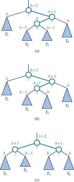
Figure 11.12: Rebalancing of a subtree during a typical insertion into an AVL tree: (a) before the insertion; (b) after an insertion in subtree T₃ causes imbalance at z; (c) after restoring balance with trinode restructuring. Notice that the overall height of the subtree after the insertion is the same as before the insertion.

Deletion

Recall that a deletion from a regular binary search tree results in the structural removal of a node having either zero or one internal children. Such a change may violate the height-balance property in an AVL tree. In particular, if position p represents a (possibly external) child of the removed node in tree T, there may be an unbalanced node on the path from p to the root of T. (See Figure 11.13a.) In fact, there can be at most one such unbalanced node. (The justification of this fact is left as Exercise C-11.41.)

Figure 11.13: Deletion of the entry with key 32 from the AVL tree of Figure 11.11b: (a) after removing the node storing key 32, the root becomes unbalanced; (b) a trinode restructuring of x, y, and z restores the height-balance property.

As with insertion, we use trinode restructuring to restore balance in the tree T. In particular, let z be the first unbalanced position encountered going up from p toward the root of T, and let y be that child of z with greater height (y will not be an ancestor of p). Furthermore, let x be the child of y defined as follows: if one of the children of y is taller than the other, let x be the taller child of y; else (both children of y have the same height), let x be the child of y on the same side as y (that is, if y is the left child of z, let x be the left child of y, else let x be the right child of y). We then perform a restructure(x) operation. (See Figure 11.13b.)

The restructured subtree is rooted at the middle position denoted as b in the description of the trinode restructuring operation. The height-balance property is guaranteed to be locally restored within the subtree of b. (See Exercises R-11.11 and R-11.12.) Unfortunately, this trinode restructuring may reduce the height of the subtree rooted at b by 1, which may cause an ancestor of b to become unbalanced. So, after rebalancing z, we continue walking up T looking for unbalanced positions. If we find another, we perform a restructure operation to restore its balance, and continue marching up T looking for more, all the way to the root. Since the height of T is O(logn), where n is the number of entries, by Proposition 11.1, O(logn) trinode restructurings are sufficient to restore the height-balance property.

Performance of AVL Trees

By Proposition 11.1, the height of an AVL tree with n entries is guaranteed to be O(logn). Because the standard binary search-tree operation had running times bounded by the height (see Table 11.1), and because the additional work in maintaining balance factors and restructuring an AVL tree can be bounded by the length of a path in the tree, the traditional map operations run in worst-case logarithmic time with an AVL tree. We summarize these results in Table 11.2, and illustrate this performance in Figure 11.14.

Method	Running Time
size, isEmpty	O(1)
get, put, remove	O(logn)
firstEntry, lastEntry	O(logn)
ceilingEntry, floorEntry, lowerEntry, higherEntry	O(logn)
subMap	O(s + logn)
entrySet, keySet, values	O(n)

Table 11.2: Worst-case running times of operations for an n-entry sorted map realized as an AVL tree T, with s denoting the number of entries reported by subMap.

Figure 11.14: Illustrating the running time of searches and updates in an AVL tree. The time performance is O(1) per level, broken into a down phase, which typically involves searching, and an up phase, which typically involves updating height values and performing local trinode restructurings (rotations).

11.3.2 Java Implementation

A complete implementation of an AVLTreeMap class is provided in Code Fragments 11.11 and 11.12. It inherits from the standard TreeMap class and relies on the balancing framework described in Section 11.2.1. We highlight two important aspects of our implementation. First, the AVLTreeMap uses the node's auxiliary balancing variable to store the height of the subtree rooted at that node, with leaves having a balance factor of 0 by default. We also provide several utilities involving heights of nodes (see Code Fragment 11.11).

To implement the core logic of the AVL balancing strategy, we define a utility, named rebalance, that suffices to restore the height-balance property after an insertion or a deletion (see Code Fragment 11.11). Although the inherited behaviors for insertion and deletion are quite different, the necessary post-processing for an AVL tree can be unified. In both cases, we trace an upward path from the position p at which the change took place, recalculating the height of each position based on the (updated) heights of its children. We perform a trinode restructuring operation if an imbalanced position is reached. The upward march from p continues until we reach an ancestor with height that was unchanged by the map operation, or with height that was restored to its previous value by a trinode restructuring operation, or until reaching the root of the tree (in which case the overall height of the tree has increased by one). To easily detect the stopping condition, we record the “old” height of a position, as it existed before the insertion or deletion operation begin, and compare that to the newly calculated height after a possible restructuring.

Code Fragment 11.11: AVLTreeMap class. (Continues in Code Fragment 11.12.)

Code Fragment 11.12: AVLTreeMap class (continued from Code Fragment 11.11).

11.4 Splay Trees

The next search-tree structure we study is known as a a splay tree. This structure is conceptually quite different from the other balanced search trees we will discuss in this chapter, for a splay tree does not strictly enforce a logarithmic upper bound on the height of the tree. In fact, no additional height, balance, or other auxiliary data need be stored with the nodes of this tree.

The efficiency of splay trees is due to a certain move-to-root operation, called splaying, that is performed at the bottommost position p reached during every insertion, deletion, or even a search. (In essence, this is a variant of the move-to-front heuristic that we explored for lists in Section 7.7.2.) Intuitively, a splay operation causes more frequently accessed elements to remain nearer to the root, thereby reducing the typical search times. The surprising thing about splaying is that it allows us to guarantee a logarithmic amortized running time, for insertions, deletions, and searches.

11.4.1 Splaying

Given a node x of a binary search tree T, we splay x by moving x to the root of T through a sequence of restructurings. The particular restructurings we perform are important, for it is not sufficient to move x to the root of T by just any sequence of restructurings. The specific operation we perform to move x up depends upon the relative positions of x, its parent y, and x's grandparent z (if it exists). There are three cases that we will consider.

zig-zig: The node x and its parent y are both left children or both right children. (See Figure 11.15.) We promote x, making y a child of x and z a child of y, while maintaining the inorder relationships of the nodes in T.

Figure 11.15: Zig-zig: (a) before; (b) after. There is another symmetric configuration where x and y are left children.

zig-zag: One of x and y is a left child and the other is a right child. (See Figure 11.16.) In this case, we promote x by making x have y and z as its children, while maintaining the inorder relationships of the nodes in T.

Figure 11.16: Zig-zag: (a) before; (b) after. There is another symmetric configuration where x is a right child and y is a left child.

zig: x does not have a grandparent. (See Figure 11.17.) In this case, we perform a single rotation to promote x over y, making y a child of x, while maintaining the relative inorder relationships of the nodes in T.

Figure 11.17: Zig: (a) before; (b) after. There is another symmetric configuration where x is originally a left child of y.

We perform a zig-zig or a zig-zag when x has a grandparent, and we perform a zig when x has a parent but not a grandparent. A splaying step consists of repeating these restructurings at x until x becomes the root of T. An example of the splaying of a node is shown in Figures 11.18 and 11.19.

Figure 11.18: Example of splaying a node: (a) splaying the node storing 14 starts with a zig-zag; (b) after the zig-zag; (c) the next step will be a zig-zig. (Continues in Figure 11.19.)

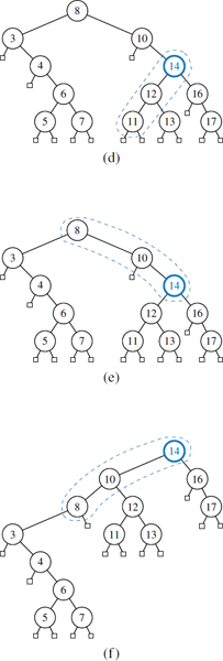
Figure 11.19: Example of splaying a node:(d) after the zig-zig; (e) the next step is again a zig-zig; (f) after the zig-zig. (Continued from Figure 11.18.)

11.4.2 When to Splay

The rules that dictate when splaying is performed are as follows:

• When searching for key k, if k is found at position p, we splay p, else we splay the parent of the leaf position at which the search terminates unsuccessfully. For example, the splaying in Figures 11.18 and 11.19 would be performed after searching successfully for key 14 or unsuccessfully for key 15.
• When inserting key k, we splay the newly created internal node where k gets inserted. For example, the splaying in Figures 11.18 and 11.19 would be performed if 14 were the newly inserted key. We show a sequence of insertions in a splay tree in Figure 11.20.

  

  Figure 11.20: A sequence of insertions in a splay tree: (a) initial tree; (b) after inserting 3, but before a zig step; (c) after splaying; (d) after inserting 2, but before a zig-zag step; (e) after splaying; (f) after inserting 4, but before a zig-zig step; (g) after splaying.

• When deleting a key k, we splay the position p that is the parent of the removed node; recall that by the removal algorithm for binary search trees, the removed node may be that originally containing k, or a descendant node with a replacement key. An example of splaying following a deletion is shown in Figure 11.21.

Figure 11.21: Deletion from a splay tree: (a) the deletion of 8 from the root node is performed by moving to the root the key of its inorder predecessor w, deleting w, and splaying the parent p of w; (b) splaying p starts with a zig-zig; (c) after the zig-zig; (d) the next step is a zig; (e) after the zig.

11.4.3 Java Implementation

Although the mathematical analysis of a splay tree's performance is complex (see Section 11.4.4), the implementation of splay trees is a rather simple adaptation to a standard binary search tree. Code Fragment 11.13 provides a complete implementation of a SplayTreeMap class, based upon the underlying TreeMap class and use of the balancing framework described in Section 11.2.1. Note that the original TreeMap class makes calls to the rebalanceAccess method, not just from within the get method, but also within the put method when modifying the value associated with an existing key, and within a failed remove operation.

Code Fragment 11.13: A complete implementation of the SplayTreeMap class.

11.4.4 Amortized Analysis of Splaying

After a zig-zig or zig-zag, the depth of position p decreases by two, and after a zig the depth of p decreases by one. Thus, if p has depth d, splaying p consists of a sequence of zig-zigs and/or zig-zags, plus one final zig if d is odd. Since a single zig-zig, zig-zag, or zig affects a constant number of nodes, it can be done in O(1) time. Thus, splaying a position p in a binary search tree T takes time O(d), where d is the depth of p in T. In other words, the time for performing a splaying step for a position p is asymptotically the same as the time needed just to reach that position in a top-down search from the root of T.

Worst-Case Time

In the worst case, the overall running time of a search, insertion, or deletion in a splay tree of height h is O(h), since the position we splay might be the deepest position in the tree. Moreover, it is possible for h to be as large as n, as shown in Figure 11.20. Thus, from a worst-case point of view, a splay tree is not an attractive data structure.

In spite of its poor worst-case performance, a splay tree performs well in an amortized sense. That is, in a sequence of intermixed searches, insertions, and deletions, each operation takes on average logarithmic time. We perform the amortized analysis of splay trees using the accounting method.

Amortized Performance of Splay Trees

For our analysis, we note that the time for performing a search, insertion, or deletion is proportional to the time for the associated splaying. So let us consider only splaying time.

Let T be a splay tree with n keys, and let w be a node of T. We define the size n(w) of w as the number of nodes in the subtree rooted at w. Note that this definition implies that the size of an internal node is one more than the sum of the sizes of its children. We define the rank r(w) of a node w as the logarithm in base 2 of the size of w, that is, r(w) = log(n(w)). Clearly, the root of T has the maximum size, n, and the maximum rank, logn, while each leaf has size 1 and rank 0.

We use cyber-dollars to pay for the work we perform in splaying a position p in T, and we assume that one cyber-dollar pays for a zig, while two cyber-dollars pay for a zig-zig or a zig-zag. Hence, the cost of splaying a position at depth d is d cyber-dollars. We keep a virtual account storing cyber-dollars at each position of T. Note that this account exists only for the purpose of our amortized analysis, and does not need to be included in a data structure implementing the splay tree T.

An Accounting Analysis of Splaying

When we perform a splaying, we pay a certain number of cyber-dollars (the exact value of the payment will be determined at the end of our analysis). We distinguish three cases:

• If the payment is equal to the splaying work, then we use it all to pay for the splaying.
• If the payment is greater than the splaying work, we deposit the excess in the accounts of several nodes.
• If the payment is less than the splaying work, we make withdrawals from the accounts of several nodes to cover the deficiency.

We show below that a payment of O(logn) cyber-dollars per operation is sufficient to keep the system working, that is, to ensure that each node keeps a nonnegative account balance.

An Accounting Invariant for Splaying

We use a scheme in which transfers are made between the accounts of the nodes to ensure that there will always be enough cyber-dollars to withdraw for paying for splaying work when needed.

In order to use the accounting method to perform our analysis of splaying, we maintain the following invariant:

Note that the invariant is “financially sound,” since it does not require us to make a preliminary deposit to endow a tree with zero keys.

Let r(T) be the sum of the ranks of all the nodes of T. To preserve the invariant after a splaying, we must make a payment equal to the splaying work plus the total change in r(T). We refer to a single zig, zig-zig, or zig-zag operation in a splaying as a splaying substep. Also, we denote the rank of a node w of T before and after a splaying substep with r(w) and r′(w), respectively. The following proposition gives an upper bound on the change of r(T) caused by a single splaying substep. We will repeatedly use this lemma in our analysis of a full splaying of a node to the root.

Proposition 11.2: Let δ be the variation of r(T) caused by a single splaying sub-step (a zig, zig-zig, or zig-zag) for a node x in T. We have the following:

• δ ≤ 3(r′ (x) − r(x)) − 2 if the substep is a zig-zig or zig-zag.
• δ ≤ 3(r′ (x) − r(x)) if the substep is a zig.

Justification: We use the fact that, if a > 0, b > 0, and c > a + b,

Let us consider the change in r(T) caused by each type of splaying substep.

zig-zig: (Recall Figure 11.15.) Since the size of each node is one more than the size of its two children, note that only the ranks of x, y, and z change in a zig-zig operation, where y is the parent of x and z is the parent of y. Also, r′(x) = r(z), r′(y) ≤ r′(x), and r(x) ≤ r(y). Thus,

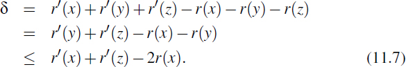
Note that n(x) + n′(z) < n′(x). Thus, r(x) + r′(z) < 2r′(x) − 2, as per Formula 11.6; that is,

r′(z) < 2r′ (x) − r(x) − 2.

This inequality and Formula 11.7 imply

zig-zag: (Recall Figure 11.16.) Again, by the definition of size and rank, only the ranks of x, y, and z change, where y denotes the parent of x and z denotes the parent of y. Also, r(x) < r(y) < r(z) = r′(x). Thus,

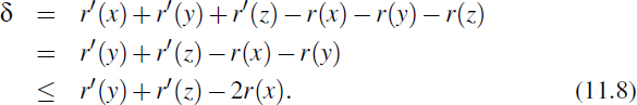
Note that n′(y) + n′(z) < n′(x); hence, r′(y) + r′(z) < 2r′(x) − 2, as per Formula 11.6. Thus,

zig: (Recall Figure 11.17.) In this case, only the ranks of x and y change, where y denotes the parent of x. Also, r′(y) ≤ r(y) and r′(x) ≥ r(x). Thus,

Proposition 11.3: Let T be a splay tree with root t, and let Δ be the total variation of r(T) caused by splaying a node x at depth d. We have

Justification: Splaying node x consists of splaying substeps, each of which is a zig-zig or a zig-zag, except possibly the last one, which is a zig if d is odd. Let r₀(x) = r(x) be the initial rank of x, and for i = 1,...,c, let r_i(x) be the rank of x after the i^th substep and δ_i be the variation of r(T) caused by the i^th substep. By Proposition 11.2, the total variation Δ of r(T) caused by splaying x is

By Proposition 11.3, if we make a payment of 3(r(t) − r(x)) + 2 cyber-dollars towards the splaying of node x, we have enough cyber-dollars to maintain the invariant, keeping r(w) cyber-dollars at each node w in T, and pay for the entire splaying work, which costs d cyber-dollars. Since the size of the root t is n, its rank r(t) = logn. Given that r(x) ≥ 0, the payment to be made for splaying is O(logn) cyber-dollars. To complete our analysis, we have to compute the cost for maintaining the invariant when a node is inserted or deleted.

When inserting a new node w into a splay tree with n keys, the ranks of all the ancestors of w are increased. Namely, let w₀,w_i,...,w_d be the ancestors of w, where w₀ = w, w_i is the parent of w_i−1, and w_d is the root. For i = 1,..., d, let n′(w_i) and n(w_i) be the size of w_i before and after the insertion, respectively, and let r′(w_i) and r(w_i) be the rank of w_i before and after the insertion. We have

n′(w_i) = n(w_i) + 1.

Also, since n(w_i) + 1 ≤ n(w_i+1), for i = 0,1,...,d − 1, we have the following for each i in this range:

r′(w_i) = log(n′(w_i)) = log(n(w_i) + 1) ≤ log(n(w_i+1)) = r(w_i+1).

Thus, the total variation of r(T) caused by the insertion is

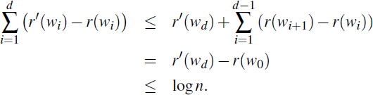
Therefore, a payment of O(logn) cyber-dollars is sufficient to maintain the invariant when a new node is inserted.

When deleting a node w from a splay tree with n keys, the ranks of all the ancestors of w are decreased. Thus, the total variation of r(T) caused by the deletion is negative, and we do not need to make any payment to maintain the invariant when a node is deleted. Therefore, we may summarize our amortized analysis in the following proposition (which is sometimes called the “balance proposition” for splay trees):

Proposition 11.4: Consider a sequence of m operations on a splay tree, each one a search, insertion, or deletion, starting from a splay tree with zero keys. Also, let n_i be the number of keys in the tree after operation i, and n be the total number of insertions. The total running time for performing the sequence of operations is

which is O(mlogn).

In other words, the amortized running time of performing a search, insertion, or deletion in a splay tree is O(logn), where n is the size of the splay tree at the time. Thus, a splay tree can achieve logarithmic-time amortized performance for implementing a sorted map ADT. This amortized performance matches the worst-case performance of AVL trees, (2,4) trees, and red-black trees, but it does so using a simple binary tree that does not need any extra balance information stored at each of its nodes. In addition, splay trees have a number of other interesting properties that are not shared by these other balanced search trees. We explore one such additional property in the following proposition (which is sometimes called the “Static Optimality” proposition for splay trees):

Proposition 11.5: Consider a sequence of m operations on a splay tree, each one a search, insertion, or deletion, starting from a splay tree T with zero keys. Also, let f(i) denote the number of times the entry i is accessed in the splay tree, that is, its frequency, and let n denote the total number of entries. Assuming that each entry is accessed at least once, then the total running time for performing the sequence of operations is

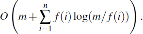
We omit the proof of this proposition, but it is not as hard to justify as one might imagine. The remarkable thing is that this proposition states that the amortized running time of accessing an entry i is O(log(m/f(i))).

11.5 (2,4) Trees

In this section, we will consider a data structure known as a (2,4) tree. It is a particular example of a more general structure known as a multiway search tree, in which internal nodes may have more than two children. Other forms of multiway search trees will be discussed in Section 15.3.

11.5.1 Multiway Search Trees

Recall that general trees are defined so that internal nodes may have many children. In this section, we discuss how general trees can be used as multiway search trees. Map entries stored in a search tree are pairs of the form (k, v), where k is the key and v is the value associated with the key.

Definition of a Multiway Search Tree

Let w be a node of an ordered tree. We say that w is a d-node if w has d children. We define a multiway search tree to be an ordered tree T that has the following properties, which are illustrated in Figure 11.22a:

• Each internal node of T has at least two children. That is, each internal node is a d-node such that d ≥ 2.
• Each internal d-node w of T with children c₁,..., c_d stores an ordered set of d − 1 key-value pairs (k₁, v₁),..., (k_d−1, v_d−1), where k₁ ≤ ··· ≤ k_d−1.
• Let us conventionally define k₀ = −∞ and k_d = +∞. For each entry (k, v) stored at a node in the subtree of w rooted at c_i, i = 1,..., d, we have that k_i−1 ≤ k ≤ k_i.

That is, if we think of the set of keys stored at w as including the special fictitious keys k₀ = −∞ and k_d = +∞, then a key k stored in the subtree of T rooted at a child node c_i must be “in between” two keys stored at w. This simple viewpoint gives rise to the rule that a d-node stores d − 1 regular keys, and it also forms the basis of the algorithm for searching in a multiway search tree.

By the above definition, the external nodes of a multiway search do not store any data and serve only as “placeholders.” As with our convention for binary search trees (Section 11.1), these can be replaced by null references in practice. A binary search tree can be viewed as a special case of a multiway search tree, where each internal node stores one entry and has two children.

Whether internal nodes of a multiway tree have two children or many, however, there is an interesting relationship between the number of key-value pairs and the number of external nodes in a multiway search tree.

Proposition 11.6: An n-entry multiway search tree has n + 1 external nodes.

We leave the justification of this proposition as an exercise (C-11.49).

Figure 11.22: (a) A multiway search tree T; (b) search path in T for key 12 (unsuccessful search); (c) search path in T for key 24 (successful search).

Searching in a Multiway Tree

Searching for an entry with key k in a multiway search tree T is simple. We perform such a search by tracing a path in T starting at the root. (See Figure 11.22b and c.) When we are at a d-node w during this search, we compare the key k with the keys k₁,..., k_d−1 stored at w. If k = k_i for some i, the search is successfully completed. Otherwise, we continue the search in the child c_i of w such that k_i−1 < k < k_i. (Recall that we conventionally define k₀ = −∞ and k_d = +∞.) If we reach an external node, then we know that there is no entry with key k in T, and the search terminates unsuccessfully.

Data Structures for Representing Multiway Search Trees

In Section 8.3.3, we discuss a linked data structure for representing a general tree. This representation can also be used for a multiway search tree. When using a general tree to implement a multiway search tree, we must store at each node one or more key-value pairs associated with that node. That is, we need to store with w a reference to some collection that stores the entries for w.

During a search for key k in a multiway search tree, the primary operation needed when navigating a node is finding the smallest key at that node that is greater than or equal to k. For this reason, it is natural to model the information at a node itself as a sorted map, allowing use of the ceilingEntry(k) method. We say such a map serves as a secondary data structure to support the primary data structure represented by the entire multiway search tree. This reasoning may at first seem like a circular argument, since we need a representation of a (secondary) ordered map to represent a (primary) ordered map. We can avoid any circular dependence, however, by using the bootstrapping technique, where we use a simple solution to a problem to create a new, more advanced solution.

In the context of a multiway search tree, a natural choice for the secondary structure at each node is the SortedTableMap of Section 10.3.1. Because we want to determine the associated value in case of a match for key k, and otherwise the corresponding child c_i such that k_i−1 < k < k_i, we recommend having each key k_i in the secondary structure map to the pair (v_i, c_i). With such a realization of a multiway search tree T, processing a d-node w while searching for an entry of T with key k can be performed using a binary search operation in O(logd) time. Let d_max denote the maximum number of children of any node of T, and let h denote the height of T. The search time in a multiway search tree is therefore O(hlogd_max). If d_max is a constant, the running time for performing a search is O(h).

The primary efficiency goal for a multiway search tree is to keep the height as small as possible. We will next discuss a strategy that caps d_max at 4 while guaranteeing a height h that is logarithmic in n, the total number of entries stored in the map.

11.5.2 (2,4)-Tree Operations

One form of a multiway search tree that keeps the tree balanced while using small secondary data structures at each node is the (2, 4) tree, also known as a 2-4 tree or 2-3-4 tree. This data structure achieves these goals by maintaining two simple properties (see Figure 11.23):

Size Property: Every internal node has at most four children.

Depth Property: All the external nodes have the same depth.

Figure 11.23: A (2,4) tree.

Again, we assume that external nodes are empty and, for the sake of simplicity, we describe our search and update methods assuming that external nodes are real nodes, although this latter requirement is not strictly needed.

Enforcing the size property for (2,4) trees keeps the nodes in the multiway search tree simple. It also gives rise to the alternative name “2-3-4 tree,” since it implies that each internal node in the tree has 2, 3, or 4 children. Another implication of this rule is that we can represent the secondary map stored at each internal node using an unordered list or an ordered array, and still achieve O(1)-time performance for all operations (since d_max = 4). The depth property, on the other hand, enforces an important bound on the height of a (2,4) tree.

Proposition 11.7: The height of a (2,4) tree storing n entries is O(log n).

Justification: Let h be the height of a (2,4) tree T storing n entries. We justify the proposition by showing the claim

To justify this claim note first that, by the size property, we can have at most 4 nodes at depth 1, at most 4² nodes at depth 2, and so on. Thus, the number of external nodes in T is at most 4^h. Likewise, by the depth property and the definition of a (2,4) tree, we must have at least 2 nodes at depth 1, at least 2² nodes at depth 2, and so on. Thus, the number of external nodes in T is at least 2^h. In addition, by Proposition 11.6, the number of external nodes in T is n + 1. Therefore, we obtain

2^h ≤ n + 1 ≤ 4^h.

Taking the logarithm in base 2 of the terms for the above inequalities, we get that

h ≤ log(n + 1) ≤ 2h,

which justifies our claim (Formula 11.9) when terms are rearranged.

Proposition 11.7 states that the size and depth properties are sufficient for keeping a multiway tree balanced. Moreover, this proposition implies that performing a search in a (2,4) tree takes O(logn) time and that the specific realization of the secondary structures at the nodes is not a crucial design choice, since the maximum number of children d_max is a constant.

Maintaining the size and depth properties requires some effort after performing insertions and deletions in a (2,4) tree, however. We discuss these operations next.

Insertion

To insert a new entry (k, v), with key k, into a (2,4) tree T, we first perform a search for k. Assuming that T has no entry with key k, this search terminates unsuccessfully at an external node z. Let w be the parent of z. We insert the new entry into node w and add a new child y (an external node) to w on the left of z.

Our insertion method preserves the depth property, since we add a new external node at the same level as existing external nodes. Nevertheless, it may violate the size property. Indeed, if a node w was previously a 4-node, then it would become a 5-node after the insertion, which causes the tree T to no longer be a (2,4) tree. This type of violation of the size property is called an overflow at node w, and it must be resolved in order to restore the properties of a (2,4) tree. Let c₁,..., c₅ be the children of w, and let k₁,..., k₄ be the keys stored at w. To remedy the overflow at node w, we perform a split operation on w as follows (see Figure 11.24):

• Replace w with two nodes w′ and w″, where
  • w′ is a 3-node with children c₁, c₂, c₃ storing keys k₁ and k₂.
  • w″ is a 2-node with children c₄, c₅ storing key k₄.
• If w is the root of T, create a new root node u; else, let u be the parent of w.
• Insert key k₃ into u and make w' and w″ children of u, so that if w was child i of u, then w' and w″ become children i and i + 1 of u, respectively.

As a consequence of a split operation on node w, a new overflow may occur at the parent u of w. If such an overflow occurs, it triggers in turn a split at node u. (See Figure 11.25.) A split operation either eliminates the overflow or propagates it into the parent of the current node. We show a sequence of insertions in a (2,4) tree in Figure 11.26.

Figure 11.24: A node split: (a) overflow at a 5-node w; (b) the third key of w inserted into the parent u of w; (c) node w replaced with a 3-node w′ and a 2-node w″.

Figure 11.25: An insertion in a (2,4) tree that causes a cascading split: (a) before the insertion; (b) insertion of 17, causing an overflow; (c) a split; (d) after the split a new overflow occurs; (e) another split, creating a new root node; (f) final tree.

Figure 11.26: A sequence of insertions into a (2,4) tree: (a) initial tree with one entry; (b) insertion of 6; (c) insertion of 12; (d) insertion of 15, which causes an overflow; (e) split, which causes the creation of a new root node; (f) after the split; (g) insertion of 3; (h) insertion of 5, which causes an overflow; (i) split; (j) after the split; (k) insertion of 10; (l) insertion of 8.

Analysis of Insertion in a (2,4) Tree

Because d_max is at most 4, the original search for the placement of new key k uses O(1) time at each level, and thus O(logn) time overall, since the height of the tree is O(logn) by Proposition 11.7.

The modifications to a single node to insert a new key and child can be implemented to run in O(1) time, as can a single split operation. The number of cascading split operations is bounded by the height of the tree, and so that phase of the insertion process also runs in O(logn) time. Therefore, the total time to perform an insertion in a (2,4) tree is O(logn).

Deletion

Let us now consider the removal of an entry with key k from a (2,4) tree T. We begin such an operation by performing a search in T for an entry with key k. Removing an entry from a (2,4) tree can always be reduced to the case where the entry to be removed is stored at a node w whose children are external nodes. Suppose, for instance, that the entry with key k that we wish to remove is stored in the i^th entry (k_i, v_i) at a node z that has internal children. In this case, we swap the entry (k_i, v_i) with an appropriate entry that is stored at a node w with external children as follows (see Figure 11.27d):

1. We find the rightmost internal node w in the subtree rooted at the i^th child of z, noting that the children of node w are all external nodes.
2. We swap the entry (k_i, v_i) at z with the last entry of w.

Once we ensure that the entry to remove is stored at a node w with only external children (because either it was already at w or we swapped it into w), we simply remove the entry from w and remove the external node that is the i^th child of w.

Removing an entry (and a child) from a node w as described above preserves the depth property, for we always remove an external child from a node w with only external children. However, in removing such an external node, we may violate the size property at w. Indeed, if w was previously a 2-node, then it becomes a 1-node with no entries after the removal (Figure 11.27a and d), which is not allowed in a (2,4) tree. This type of violation of the size property is called an underflow at node w. To remedy an underflow, we check whether an immediate sibling of w is a 3-node or a 4-node. If we find such a sibling s, then we perform a transfer operation, in which we move a child of s to w, a key of s to the parent u of w and s, and a key of u to w. (See Figure 11.27b and c.) If w has only one sibling, or if both immediate siblings of w are 2-nodes, then we perform a fusion operation, in which we merge w with a sibling, creating a new node w′, and move a key from the parent u of w to w'. (See Figure 11.27e and f.)

Figure 11.27: A sequence of removals from a (2,4) tree: (a) removal of 4, causing an underflow; (b) a transfer operation; (c) after the transfer operation; (d) removal of 12, causing an underflow; (e) a fusion operation; (f) after the fusion operation; (g) removal of 13; (h) after removing 13.

A fusion operation at node w may cause a new underflow to occur at the parent u of w, which in turn triggers a transfer or fusion at u. (See Figure 11.28.) Hence, the number of fusion operations is bounded by the height of the tree, which is O(logn) by Proposition 11.7. If an underflow propagates all the way up to the root, then the root is simply deleted. (See Figure 11.28c and d.)

Figure 11.28: A propagating sequence of fusions in a (2,4) tree: (a) removal of 14, which causes an underflow; (b) fusion, which causes another underflow; (c) second fusion operation, which causes the root to be removed; (d) final tree.

Performance of (2,4) Trees

The asymptotic performance of a (2,4) tree is identical to that of an AVL tree (see Table 11.2) in terms of the sorted map ADT, with guaranteed logarithmic bounds for most operations. The time complexity analysis for a (2,4) tree having n key-value pairs is based on the following:

• The height of a (2,4) tree storing n entries is O(logn), by Proposition 11.7.
• A split, transfer, or fusion operation takes O(1) time.
• A search, insertion, or removal of an entry visits O(logn) nodes.

Thus, (2,4) trees provide for fast map search and update operations. (2,4) trees also have an interesting relationship to the data structure we discuss next.

11.6 Red-Black Trees

Although AVL trees and (2, 4) trees have a number of nice properties, they also have some disadvantages. For instance, AVL trees may require many restructure operations (rotations) to be performed after a deletion, and (2,4) trees may require many split or fusing operations to be performed after an insertion or removal. The data structure we discuss in this section, the red-black tree, does not have these drawbacks; it uses O(1) structural changes after an update in order to stay balanced.

Formally, a red-black tree is a binary search tree (see Section 11.1) with nodes colored red and black in a way that satisfies the following properties:

Root Property: The root is black.

External Property: Every external node is black.

Red Property: The children of a red node are black.

Depth Property: All external nodes have the same black depth, defined as the number of proper ancestors that are black.

An example of a red-black tree is shown in Figure 11.29.

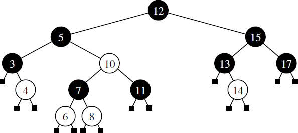
Figure 11.29: An example of a red-black tree, with “red” nodes drawn in white. The common black depth for this tree is 3.

We can make the red-black tree definition more intuitive by noting an interesting correspondence between red-black trees and (2,4) trees. Namely, given a red-black tree, we can construct a corresponding (2,4) tree by merging every red node w into its parent, storing the entry from w at its parent, and with the children of w becoming ordered children of the parent. For example, the red-black tree in Figure 11.29 corresponds to the (2,4) tree from Figure 11.23, as illustrated in Figure 11.30. The depth property of the red-black tree corresponds to the depth property of the (2,4) tree since exactly one black node of the red-black tree contributes to each node of the corresponding (2,4) tree.

Figure 11.30: An illustration of the correspondance between the red-black tree of Figure 11.29 and the (2,4) tree of Figure 11.23, based on the highlighted grouping of red nodes with their black parents.

Conversely, we can transform any (2,4) tree into a corresponding red-black tree by coloring each node w black and then performing the following transformations, as illustrated in Figure 11.31.

• If w is a 2-node, then keep the (black) children of w as is.
• If w is a 3-node, then create a new red node y, give w's last two (black) children to y, and make the first child of w and y be the two children of w.
• If w is a 4-node, then create two new red nodes y and z, give w's first two (black) children to y, give w's last two (black) children to z, and make y and z be the two children of w.

Notice that a red node always has a black parent in this construction.

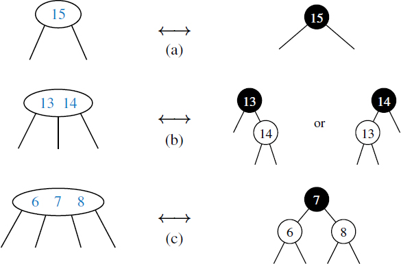
Figure 11.31: Correspondence between nodes of a (2,4) tree and a red-black tree: (a) 2-node; (b) 3-node; (c) 4-node.

Proposition 11.8: The height of a red-black tree storing n entries is O(logn).

Justification: Let T be a red-black tree storing n entries, and let h be the height of T. We justify this proposition by establishing the following fact:

log(n + 1) ≤ h ≤ 2log(n + 1).

Let d be the common black depth of all the external nodes of T. Let T′ be the (2,4) tree associated with T, and let h′ be the height of T′. Because of the correspondence between red-black trees and (2,4) trees, we know that h′ = d. Hence, by Proposition 11.7, d = h′; ≤ log(n + 1). By the red property, h ≤ 2d. Thus, we obtain h ≤ 2log(n + 1). The other inequality, log(n + 1) ≤ h, follows from Proposition 8.7 and the fact that T has n internal nodes.

11.6.1 Red-Black Tree Operations

The algorithm for searching in a red-black tree T is the same as that for a standard binary search tree (Section 11.1). Thus, searching in a red-black tree takes time proportional to the height of the tree, which is O(logn) by Proposition 11.8.

The correspondence between (2,4) trees and red-black trees provides important intuition that we will use in our discussion of how to perform updates in red-black trees; in fact, the update algorithms for red-black trees can seem mysteriously complex without this intuition. Split and fuse operations of a (2,4) tree will be effectively mimicked by recoloring neighboring red-black tree nodes. A rotation within a red-black tree will be used to change orientations of a 3-node between the two forms shown in Figure 11.31(b).

Insertion

Consider the insertion of a key-value pair (k, v) into a red-black tree T. The algorithm initially proceeds as in a standard binary search tree (Section 11.1.2). Namely, we search for k in T and if we reach an external node, we replace this node with an internal node x, storing the entry and having two external children. If this is the first entry in T, and thus x is the root, we color it black. In all other cases, we color x red. That action corresponds to inserting (k, v) into a node of the (2,4) tree T′ at the lowest internal level. The insertion preserves the root and depth properties of T, but it may violate the red property. Indeed, if x is not the root of T and its parent y is red, then we have a parent and a child (namely, y and x) that are both red. Note that by the root property, y cannot be the root of T, and by the red property (which was previously satisfied), the parent z of y must be black. Since x and its parent are red, but x's grandparent z is black, we call this violation of the red property a double red at node x. To remedy a double red, we consider two cases.

Case 1: The Siblings of y is Black. (See Figure 11.32.) In this case, the double red denotes the fact that we have added the new node to a corresponding 3-node of the (2,4) tree T′, effectively creating a malformed 4-node. This formation has one red node, y, that is the parent of another red node, x; we want the two red nodes to be siblings instead. To fix this problem, we perform a trinode restructuring of T. The trinode restructuring (introduced in Section 11.2) is done by the operation restructure(x), which consists of the following steps (see again Figure 11.32):

• Take node x, its parent y, and grandparent z, and temporarily relabel them as a, b, and c, in left-to-right order, so that a, b, and c will be visited in this order by an inorder tree traversal.
• Replace the grandparent z with the node labeled b, and make nodes a and c the children of b, keeping inorder relationships unchanged.

After performing the restructure(x) operation, we color b black and we color a and c red. Thus, the restructuring eliminates the double-red problem. Notice that the portion of any path through the restructured part of the tree is incident to exactly one black node, both before and after the trinode restructuring. Therefore, the black depth of the tree is unaffected.

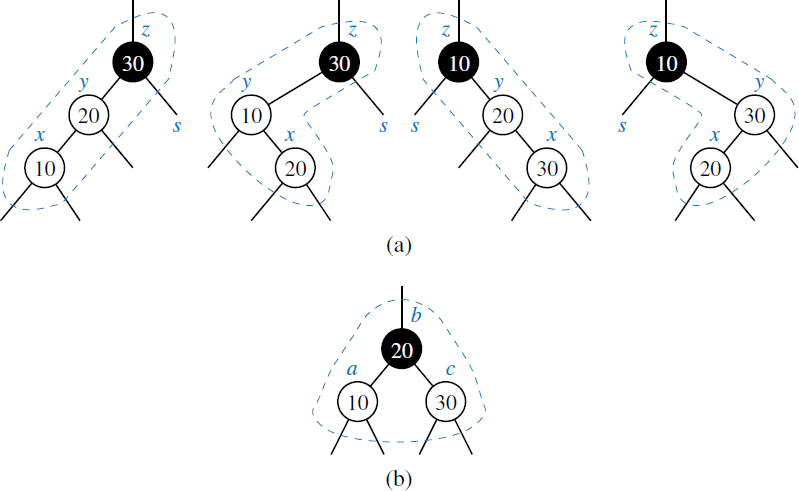
Figure 11.32: Restructuring a red-black tree to remedy a double red: (a) the four configurations for x, y, and z before restructuring; (b) after restructuring.

Case 2: The Sibling s of y is Red. (See Figure 11.33.) In this case, the double red denotes an overflow in the corresponding (2,4) tree T′. To fix the problem, we perform the equivalent of a split operation. Namely, we do a recoloring: we color y and s black and their parent z red (unless z is the root, in which case, it remains black). Notice that unless z is the root, the portion of any path through the affected part of the tree is incident to exactly one black node, both before and after the recoloring. Therefore, the black depth of the tree is unaffected by the recoloring unless z is the root, in which case it is increased by one.

However, it is possible that the double-red problem reappears after such a recoloring, albeit higher up in the tree T, since z may have a red parent. If the double-red problem reappears at z, then we repeat the consideration of the two cases at z. Thus, a recoloring either eliminates the double-red problem at node x, or propagates it to the grandparent z of x. We continue going up T performing recolorings until we finally resolve the double-red problem (with either a final recoloring or a trinode restructuring). Thus, the number of recolorings caused by an insertion is no more than half the height of tree T, that is, O(logn) by Proposition 11.8.

Figure 11.33: Recoloring to remedy the double-red problem: (a) before recoloring and the corresponding 5-node in the associated (2,4) tree before the split; (b) after recoloring and the corresponding nodes in the associated (2,4) tree after the split.

As further examples, Figures 11.34 and 11.35 show a sequence of insertion operations in a red-black tree.

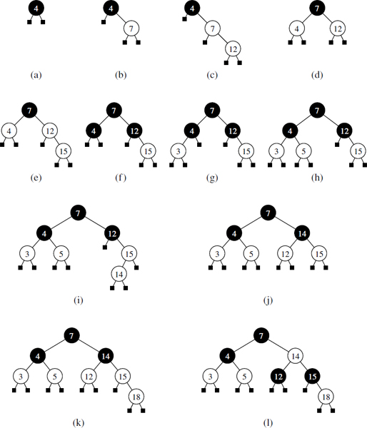
Figure 11.34: A sequence of insertions in a red-black tree: (a) initial tree; (b) insertion of 7; (c) insertion of 12, which causes a double red; (d) after restructuring; (e) insertion of 15, which causes a double red; (f) after recoloring (the root remains black); (g) insertion of 3; (h) insertion of 5; (i) insertion of 14, which causes a double red; (j) after restructuring; (k) insertion of 18, which causes a double red; (l) after recoloring. (Continues in Figure 11.35.)

Figure 11.35: A sequence of insertions in a red-black tree (continued from Figure 11.34): (m) insertion of 16, which causes a double red; (n) after restructuring; (o) insertion of 17, which causes a double red; (p) after recoloring there is again a double red, to be handled by a restructuring; (q) after restructuring.

Deletion

Deleting an entry with key k from a red-black tree T initially proceeds as for a binary search tree (Section 11.1.2). Structurally, the process results in the removal of an internal node (either that originally containing key k or its inorder predecessor) together with a child that is external, and the promotion of its other child.

If the removed internal node was red, this structural change does not affect the black depths of any paths in the tree, nor introduce any red violations, and so the resulting tree remains a valid red-black tree. In the corresponding (2,4) tree T', this case denotes the shrinking of a 4-node or 3-node. If the removed internal node was black, it must have had black height 1, and therefore either both of its children were external, or it had one red child that was an internal node with two external children. In the latter case, the removed node represents the black part of a corresponding 3-node, and we restore the red-black properties by recoloring the promoted child to be black.

The most complex case is when the removed node was black and had two external children. In the corresponding (2,4) tree, this denotes the removal of an entry from a 2-node. Without rebalancing, such a change results in a deficit of one for the black depth of the external position p that is the promoted child of the deleted internal node. To preserve the depth property, we temporarily assign the promoted leaf a fictitious double black color. A double black in T denotes an underflow in the corresponding (2,4) tree T'. To remedy a double-black problem at an arbitrary position p, we will consider three cases.

Case 1: The Sibling y of p is Black and has a Red Child x. (See Figure 11.36.) We perform a trinode restructuring, as originally described in Section 11.2. The operation restructure(x) takes the node x, its parent y, and grandparent z, labels them temporarily left to right as a, b, and c, and replaces z with the node labeled b, making it the parent of the other two. We color a and c black, and give b the former color of z.

Notice that the path to p in the result includes one additional black node after the restructure, while the number of black nodes on paths to any of the other three subtrees illustrated in Figure 11.36 remains unchanged. Therefore, we return p to be colored (regular) black, and the double-black problem is eliminated.

Resolving this case corresponds to a transfer operation in the (2,4) tree T' between two children of node z. The fact that y has a red child assures us that it represents either a 3-node or a 4-node. In effect, the entry previously stored at z is demoted to become a new 2-node to resolve the deficiency, while an entry stored at y or its child is promoted to take the place of the entry previously stored at z.

Figure 11.36: Restructuring of a red-black tree to remedy the double-black problem: (a) and (b) configurations before the restructuring, where p is a right child and the associated nodes in the corresponding (2,4) tree before the transfer (two other symmetric configurations where p is a left child are possible); (c) configuration after the restructuring and the associated nodes in the corresponding (2,4) tree after the transfer. The gray color for node z in parts (a) and (b) and for node b in part (c) denotes the fact that this node may be colored either red or black.

Case 2: The Sibling y of p is Black and Both Children of y are Black.

We do a recoloring, beginning by changing the color of p from double black to black and the color of y from black to red. This does not create any red violation, because both children of y are black. To counteract the decrease in black depth for paths passing through y or p, we consider the common parent of p and y, which we denote as z. If z is red, we color it black and the problem has been resolved (see Figure 11.37a). If z is black, we color it double black, thereby propagating the problem higher up the tree (see Figure 11.37b).

Resolving this case corresponds to a fusion operation in the corresponding (2,4) tree T′, as y must represent a 2-node. The case where the problem propagates upward is when parent z also represents a 2-node.

Figure 11.37: A recoloring operation, which has neutral effect on the black depth for paths: (a) when z is originally red, the recoloring resolves the double-black problem, ending the process; (b) when z is originally black, it becomes double-black, requiring a cascading remedy.

Case 3: Sibling y of p is Red. (See Figure 11.38.)

Let z denote the common parent of y and p, and note that z must be black, because y is red. The combination of y and z represents a 3-node in the corresponding (2,4) tree T′. In this case, we perform a rotation about y and z, and then recolor y black and z red. This denotes a reorientation of a 3-node in the corresponding (2,4) tree T′.

We now reconsider the double-black problem at p. After the adjustment, the sibling of p is black, and either Case 1 or Case 2 applies. Furthermore, the next application will be the last, because Case 1 is always terminal and Case 2 will be terminal given that the parent of p is now red.

Figure 11.38: A rotation and recoloring about red node y and black node z in the presence of a double-black problem (a symmetric configuration is possible). This amounts to a change of orientation in the corresponding 3-node of a (2,4) tree. This operation does not affect the black depth of any paths through this portion of the tree, but after the operation, one of the other resolutions to the double-black problem may be applied, as the sibling of p will be black.

In Figure 11.39, we show a sequence of deletions on a red-black tree. We illustrate a Case 1 restructuring in parts (c) and (d). We illustrate a Case 2 recoloring in parts (f) and (g). Finally, we show an example of a Case 3 rotation between parts (i) and (j), concluding with a Case 2 recoloring in part (k).

Performance of Red-Black Trees

The asymptotic performance of a red-black tree is identical to that of an AVL tree or a (2,4) tree in terms of the sorted map ADT, with guaranteed logarithmic time bounds for most operations. (See Table 11.2 for a summary of the AVL performance.) The primary advantage of a red-black tree is that an insertion or deletion requires only a constant number of restructuring operations. (This is in contrast to AVL trees and (2,4) trees, both of which require a logarithmic number of structural changes per map operation in the worst case.) That is, an insertion or deletion in a red-black tree requires logarithmic time for a search, and may require a logarithmic number of recoloring operations that cascade upward. We formalize these facts with the following propositions.

Proposition 11.9: The insertion of an entry in a red-black tree storing n entries can be done in O(logn) time and requires O(log n) recolorings and at most one trinode restructuring.

Proposition 11.10: The algorithm for deleting an entry from a red-black tree with n entries takes O(logn) time and performs O(logn) recolorings and at most two restructuring operations.

The proofs of these propositions are left as Exercises R-11.26 and R-11.27.

Figure 11.39: A sequence of deletions from a red-black tree: (a) initial tree; (b) removal of 3; (c) removal of 12, causing a black deficit to the right of 7 (handled by restructuring); (d) after restructuring; (e) removal of 17; (f) removal of 18, causing a black deficit to the right of 16 (handled by recoloring); (g) after recoloring; (h) removal of 15; (i) removal of 16, causing a black deficit to the right of 14 (handled initially by a rotation); (j) after the rotation the black deficit needs to be handled by a recoloring; (k) after the recoloring.

11.6.2 Java Implementation

In this section, we will provide an implementation of a RBTreeMap class that inherits from the standard TreeMap class and relies on the balancing framework described in Section 11.2.1. In that framework, each node stores an auxiliary integer that can be used for maintaining balance information. For a red-black tree, we use that integer to represent color, choosing to let value 0 (the default) designate the color black, and value 1 the color red; with this convention, any newly created leaf in the tree will be black.

Our implementation begins in Code Fragment 11.14, with constructors for an empty map, and a series of convenient utilities for managing the auxiliary field to represent color information. That code fragment continues with support for rebalancing the tree after an insertion is performed. When an entry has been inserted in a tree by the standard search-tree algorithm, it will be stored at a previously external node that was converted to an internal node with two new external children. The rebalancelnsert hook is then called, allowing us the opportunity to modify the tree. Except for the special case where the new element is at the root, we change the color of the node with the new element to red (it had been black when a leaf), and then we consider the possibility that we have a double-red violation. The resolveRed utility closely follows the case analysis described in Section 11.6.1, recurring in the case when the red violation is propagated upward.

Code Fragment 11.15 manages the rebalancing process after a deletion, based upon the case analysis described in Section 11.6.1. If the removed node was red, then no other action is necessary; however, if the removed node was black, we must consider a way to restore the depth property. An additional challenge is that by the time the rebalanceDelete method is called, a node has already been removed from the tree (this hook is invoked on the promoted child of that removed node). Fortunately, we can infer the properties of the removed node based upon the red-black tree properties, which were satisfied before the deletion.

In particular, let p denote the promoted child of the removed node. If a black node with a red child has been deleted, then p will be that red child; we remedy this by coloring p black. Otherwise, if p is not the root, let s denote the removed node's sibling (which will appear as p's sibling after the deletion). If the deleted node was black with two black children, we must treat p as a double black node to be remedied. This is the case if, and only if, its sibling's subtree has a black internal node (because the red-black depth property was satisfied prior to the deletion). We therefore test whether s is a black internal node, or a red internal node with an internal node as a child (which must be black due to the red property of the tree).

We are able to detect the double-black problem within the rebalanceDelete method of Code Fragment 11.15, and we rely on the recursive remedyDoubleBlack method of that code fragment to resolve the problem.

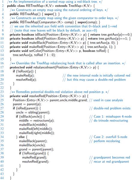
Code Fragment 11.14: The RBTreeMap class. (Continues in Code Fragment 11.15.)

Code Fragment 11.15: Support for deletion in the RBTreeMap class (continued from Code Fragment 11.14).

11.7 Exercises

Reinforcement

R-11.1	If we insert the entries (1, A), (2, B), (3, C), (4, D), and (5, E), in this order, into an initially empty binary search tree, what will it look like?
R-11.2	Insert, into an empty binary search tree, entries with keys 30, 40, 24, 58, 48, 26, 11, 13 (in this order). Draw the tree after each insertion.
R-11.3	How many different binary search trees can store the keys {1,2,3 } ?
R-11.4	Dr. Amongus claims that the order in which a fixed set of entries is inserted into a binary search tree does not matter—the same tree results every time. Give a small example that proves he is wrong.
R-11.5	Dr. Amongus claims that the order in which a fixed set of entries is inserted into an AVL tree does not matter—the same AVL tree results every time. Give a small example that proves he is wrong.
R-11.6	Our implementation of the treeSearch utility, from Code Fragment 11.3, relies on recursion. For a large unbalanced tree, it is possible that Java's call stack will reach its limit due to the recursive depth. Give an alternative implementation of that method that does not rely on the use of recursion.
R-11.7	Does the trinode restructuring in Figure 11.11 rely on a single or double rotation? What about the restructuring in Figure 11.13?
R-11.8	Draw the AVL tree resulting from the insertion of an entry with key 52 into the AVL tree of Figure 11.13b.
R-11.9	Draw the AVL tree resulting from the removal of the entry with key 62 from the AVL tree of Figure 11.13b.
R-11.10	Explain why performing a rotation in an n-node binary tree when using the array-based representation of Section 8.3.2 takes Ω(n) time.
R-11.11	Consider a deletion operation in an AVL tree that triggers a trinode restructuring for the case in which both children of the node denoted as y have equal heights. Give a schematic figure, in the style of Figure 11.12, showing the tree before and after the deletion. What is the net effect of the height of the rebalanced subtree due to the operation?
R-11.12	Repeat the previous problem, considering the case in which y's children start with different heights.
R-11.13	The rules for a deletion in an AVL tree specifically require that when the two subtrees of the node denoted as y have equal height, child x should be chosen to be “aligned” with y (so that x and y are both left children or both right children). To better understand this requirement, repeat Exercise R-11.11 assuming we picked the misaligned choice of x. Why might there be a problem in restoring the AVL property with that choice?
R-11.14	What does a splay tree look like if its entries are accessed in increasing order by their keys?
R-11.15	Perform the following sequence of operations in an initially empty splay tree and draw the tree after each set of operations. Insert keys 0, 2, 4, 6, 8, 10, 12, 14, 16, 18, in this order. Search for keys 1, 3, 5, 7, 9, 11, 13, 15, 17, 19, in this order. Delete keys 0, 2,4, 6, 8, 10, 12, 14, 16, 18, in this order.
R-11.16	The splay tree does not have good performance for the sorted map operations, because those methods lack calls to the rebalanceAccess hook. Reimplement TreeMap to include such calls.
R-11.17	Is the search tree of Figure 11.22(a) a (2,4) tree? Why or why not?
R-11.18	An alternative way of performing a split at a node w in a (2,4) tree is to partition w into w′ and w″, with w′ being a 2-node and w″ a 3-node. Which of the keys k1, k2, k3, or k4 do we store at w′s parent? Why?
R-11.19	Dr. Amongus claims that a (2,4) tree storing a set of entries will always have the same structure, regardless of the order in which the entries are inserted. Show that he is wrong.
R-11.20	Draw four different red-black trees that correspond to the same (2,4) tree.
R-11.21	Consider the set of keys K = {1,2,3,4,5,6,7,8,9,10,11,12,13,14,15}. Draw a (2,4) tree storing K as its keys using the fewest number of nodes. Draw a (2,4) tree storing K as its keys using the greatest number of nodes.
R-11.22	Consider the sequence of keys (5,16,22,45,2,10,18,30,50,12,1). Draw the result of inserting entries with these keys (in the given order) into An initially empty (2,4) tree. An initially empty red-black tree.
R-11.23	For the following statements about red-black trees, provide a justification for each true statement and a counterexample for each false one. A subtree of a red-black tree is itself a red-black tree. The sibling of an external node is either external or it is red. There is a unique (2,4) tree associated with a given red-black tree. There is a unique red-black tree associated with a given (2,4) tree.
R-11.24	Consider a tree T storing 100,000 entries. What is the worst-case height of T in the following cases? T is a binary search tree. T is an AVL tree. T is a splay tree. T is a (2,4) tree. T is a red-black tree.
R-11.25	Draw an example of a red-black tree that is not an AVL tree.
R-11.26	Give a proof of Proposition 11.9
R-11.27	Give a proof of Proposition 11.10

Creativity

C-11.28	Explain why you would get the same output in an inorder listing of the entries in a binary search tree, T, independent of whether T is maintained to be an AVL tree, splay tree, or red-black tree.
C-11.29	Explain how to use an AVL tree or a red-black tree to sort n comparable elements in O(nlogn) time in the worst case.
C-11.30	Can we use a splay tree to sort n comparable elements in O(nlogn) time in the worst case? Why or why not?
C-11.31	Implement a putlfAbsent method, as originally described in Exercise C-10.33, for the TreeMap class.
C-11.32	Show that any n-node binary tree can be converted to any other n-node binary tree using O(n) rotations.
C-11.33	For a key k that is not found in binary search tree T, prove that both the greatest key less than k and the least key greater than k lie on the path traced by the search for k.
C-11.34	In Section 11.1.4 we claim that the subMap method of a binary search tree, as implemented in Code Fragment 11.6, executes in O(s + h) time where s is the number of entries contained within the submap and h is the height of the tree. Prove this result, by arguing about the maximum number of times the recursive submethod can be called on positions that are not included within the submap.
C-11.35	Consider a sorted map that is implemented with a standard binary search tree T. Describe how to perform an operation removeSubMap(k1, k2) that removes all the entries whose keys fall within subMap(k1, k2), in worst-case time O(s + h), where s is the number of entries removed and h is the height of T.
C-11.36	Repeat the previous problem using an AVL tree, achieving a running time of O(slog n). Why doesn't the solution to the previous problem trivially result in an O(s + logn) algorithm for AVL trees?
C-11.37	Suppose we wish to support a new method countRange(k1, k2) that determines how many keys of a sorted map fall in the specified range. We could clearly implement this in O(s + h) time by adapting our approach to subMap. Describe how to modify the search-tree structure to support O(h) worst-case time for countRange.
C-11.38	If the approach described in the previous problem were implemented as part of the TreeMap class, what additional modifications (if any) would be necessary to a subclass such as AVLTreeMap in order to maintain support for the new method?
C-11.39	Draw a schematic of an AVL tree such that a single remove operation could require Ω(logn) trinode restructurings (or rotations) from a leaf to the root in order to restore the height-balance property.
C-11.40	Show that the nodes that become temporarily unbalanced in an AVL tree during an insertion may be nonconsecutive on the path from the newly inserted node to the root.
C-11.41	Show that at most one node in an AVL tree becomes temporarily unbalanced after the immediate deletion of a node as part of the standard remove map operation.
C-11.42	In our AVL implementation, each node stores the height of its subtree, which is an arbitrarily large integer. The space usage for an AVL tree can be reduced by instead storing the balance factor of a node, which is defined as the height of its left subtree minus the height of its right subtree. Thus, the balance factor of a node is always equal to −1, 0, or 1, except during an insertion or removal, when it may become temporarily equal to −2 or +2. Reimplement the AVLTreeMap class storing balance factors rather than subtree heights.
C-11.43	If we maintain a reference to the position of the leftmost node of a binary search tree, then operation firstEntry can be performed in O(1) time. Describe how the implementation of the other map methods need to be modified to maintain a reference to the leftmost position.
C-11.44	If the approach described in the previous problem were implemented as part of the TreeMap class, what additional modifications (if any) would be necessary to a subclass such as AVLTreeMap in order to accurately maintain the reference to the leftmost position?
C-11.45	Describe a modification to the binary search-tree data structure that would support the following two index-based operations for a sorted map in O(h) time, where h is the height of the tree. atIndex(i): Return the position p of the entry at index i of a sorted map. indexOf(p): Return the index i of the entry at position p of a sorted map.
C-11.46	Draw a splay tree, T1, together with the sequence of updates that produced it, and a red-black tree, T2, on the same set of ten entries, such that a preorder traversal of T1 would be the same as a preorder traversal of T2.
C-11.47	Let T and U be (2,4) trees storing n and m entries, respectively, such that all the entries in T have keys less than the keys of all the entries in U. Describe an O(logn + log m)-time method for joining T and U into a single tree that stores all the entries in T and U.
C-11.48	Let T be a red-black tree storing n entries, and let k be the key of an entry in T. Show how to construct from T, in O(logn) time, two red-black trees T′ and T″, such that T′ contains all the keys of T less than k, and T″ contains all the keys of T greater than k. This operation destroys T.
C-11.49	Prove that an n-entry multiway search tree has n + 1 external nodes.
C-11.50	The boolean indicator used to mark nodes in a red-black tree as being “red” or “black” is not strictly needed when we have distinct keys. Describe a scheme for implementing a red-black tree without adding any extra space to standard binary search-tree nodes.
C-11.51	Show that the nodes of any AVL tree T can be colored “red” and “black” so that T becomes a red-black tree.
C-11.52	The standard splaying step requires two passes, one downward pass to find the node x to splay, followed by an upward pass to splay the node x. Describe a method for splaying and searching for x in one downward pass. Each substep now requires that you consider the next two nodes in the path down to x, with a possible zig substep performed at the end. Describe how to perform the zig-zig, zig-zag, and zig steps.
C-11.53	Consider a variation of splay trees, called half-splay trees, where splaying a node at depth d stops as soon as the node reaches depth . Perform an amortized analysis of half-splay trees.
C-11.54	Describe a sequence of accesses to an n-node splay tree T, where n is odd, that results in T consisting of a single chain of nodes such that the path down T alternates between left children and right children.

Projects

P-11.55	Reimplement the TreeMap class using null references in place of explicit sentinels for the leaves of a tree.
P-11.56	Modify the TreeMap implementation to support location-aware entries. Provide methods firstEntry(), lastEntry(), findEntry(k), before(e), after(e), and remove(e), with all but the last of these returning an Entry instance, and the latter three accepting an Entry e as a parameter.
P-11.57	Perform an experimental study to compare the speed of our AVL tree, splay tree, and red-black tree implementations for various sequences of operations.
P-11.58	Redo the previous exercise, including an implementation of skip lists. (See Exercise P-10.71.)
P-11.59	Implement the Sorted Map ADT using a (2,4) tree. (See Section 10.3.)
P-11.60	Write a Java class that can take any red-black tree and convert it into its corresponding (2,4) tree and can take any (2,4) tree and convert it into its corresponding red-black tree.
P-11.61	In describing multisets and multimaps in Section 10.5.3, we describe a general approach for adapting a traditional map by storing all duplicates within a secondary container as a value in the map. Give an alternative implementation of a multimap using a binary search tree such that each entry of the map is stored at a distinct node of the tree. With the existence of duplicates, we redefine the search-tree property so that all entries in the left subtree of a position p with key k have keys that are less than or equal to k, while all entries in the right subtree of p have keys that are greater than or equal to k. Use the public interface given in Section 10.5.3.
P-11.62	Prepare an implementation of splay trees that uses top-down splaying as described in Exercise C-11.52. Perform extensive experimental studies to compare its performance to the standard bottom-up splaying implemented in this chapter.
P-11.63	The mergeable heap ADT is an extension of the priority queue ADT consisting of operations insert(k, v), min(), removeMin(), and merge(h), where the merge(h) operations performs a union of the mergeable heap h with the present one, incorporating all entries into the current one while emptying h. Describe a concrete implementation of the mergeable heap ADT that achieves O(logn) performance for all its operations, where n denotes the size of the resulting heap for the merge operation.
P-11.64	Write a program that performs a simple n-body simulation, called “Jumping Leprechauns.” This simulation involves n leprechauns, numbered 1 to n. It maintains a gold value gi for each leprechaun i, which begins with each leprechaun starting out with a million dollars worth of gold, that is, gi = 1,000,000 for each i = 1,2,..., n. In addition, the simulation also maintains, for each leprechaun, i, a place on the horizon, which is represented as a double-precision floating-point number, xi. In each iteration of the simulation, the simulation processes the leprechauns in order. Processing a leprechaun i during this iteration begins by computing a new place on the horizon for i, which is determined by the assignment xi = xi + rgi, where r is a random floating-point number between − 1 and 1. The leprechaun i then steals half the gold from the nearest leprechauns on either side of him and adds this gold to his gold value, gi. Write a program that can perform a series of iterations in this simulation for a given number, n, of leprechauns. You must maintain the set of horizon positions using a sorted map data structure described in this chapter.

Chapter Notes

Some of the data structures discussed in this chapter are extensively covered by Knuth in his Sorting and Searching book [61], and by Mehlhorn in [71]. AVL trees are due to Adel'son-Vel'skii and Landis [2], who invented this class of balanced search trees in 1962. Binary search trees, AVL trees, and hashing are described in Knuth's Sorting and Searching [61] book. Average-height analyses for binary search trees can be found in the books by Aho, Hopcroft, and Ullman [6] and Cormen, Leiserson, Rivest and Stein [25]. The handbook by Gonnet and Baeza-Yates [38] contains a number of theoretical and experimental comparisons among map implementations. Aho, Hopcroft, and Ullman [5] discuss (2,3) trees, which are similar to (2,4) trees. Red-black trees were defined by Bayer [10]. Variations and interesting properties of red-black trees are presented in a paper by Guibas and Sedgewick [42]. The reader interested in learning more about different balanced tree data structures is referred to the books by Mehlhorn [71] and Tarjan [88], and the book chapter by Mehlhorn and Tsakalidis [73]. Knuth [61] is excellent additional reading that includes early approaches to balancing trees. Splay trees were invented by Sleator and Tarjan [83] (see also [88]).