Chapter
12

Sorting and Selection

Contents

12.1 Merge-Sort

We have introduced several sorting algorithms thus far, including insertion-sort (see Sections 3.1.2, 7.6, and 9.4.1); selection-sort (see Section 9.4.1); bubble-sort (see Exercise C-7.51); and heap-sort (see Section 9.4.2). In this chapter, we will present four other sorting algorithms, called merge-sort, quick-sort, bucket-sort, and radix-sort, and then discuss the advantages and disadvantages of the various algorithms in Section 12.4.

12.1.1 Divide-and-Conquer

The first two algorithms we describe in this chapter, merge-sort and quick-sort, use recursion in an algorithmic design pattern called divide-and-conquer. We have already seen the power of recursion in describing algorithms in an elegant manner (see Chapter 5). The divide-and-conquer pattern consists of the following three steps:

1. Divide: If the input size is smaller than a certain threshold (say, one or two elements), solve the problem directly using a straightforward method and return the solution so obtained. Otherwise, divide the input data into two or more disjoint subsets.
2. Conquer: Recursively solve the subproblems associated with the subsets.
3. Combine: Take the solutions to the subproblems and merge them into a solution to the original problem.

Using Divide-and-Conquer for Sorting

We first describe the merge-sort algorithm at a high level, without focusing on whether the data is an array or linked list. (We will soon give concrete implementations for each.) To sort a sequence S with n elements using the three divide-and-conquer steps, the merge-sort algorithm proceeds as follows:

1. Divide: If S has zero or one element, return S immediately; it is already sorted. Otherwise (S has at least two elements), remove all the elements from S and put them into two sequences, S₁ and S₂, each containing about half of the elements of S; that is, S₁ contains the first elements of S, and S₂ contains the remaining elements.
2. Conquer: Recursively sort sequences S₁ and S₂.
3. Combine: Put the elements back into S by merging the sorted sequences S₁ and S₂ into a sorted sequence.

In reference to the divide step, we recall that the notation indicates the floor of x, that is, the largest integer k, such that k ≤ x. Similarly, the notation indicates the ceiling of x, that is, the smallest integer m, such that x ≤ m.

We can visualize an execution of the merge-sort algorithm by means of a binary tree T, called the merge-sort tree. Each node of T represents a recursive invocation (or call) of the merge-sort algorithm. We associate with each node v of T the sequence S that is processed by the invocation associated with v. The children of node v are associated with the recursive calls that process the subsequences S₁ and S₂ of S. The external nodes of T are associated with individual elements of S, corresponding to instances of the algorithm that make no recursive calls.

Figure 12.1 summarizes an execution of the merge-sort algorithm by showing the input and output sequences processed at each node of the merge-sort tree. The step-by-step evolution of the merge-sort tree is shown in Figures 12.2 through 12.4.

This algorithm visualization in terms of the merge-sort tree helps us analyze the running time of the merge-sort algorithm. In particular, since the size of the input sequence roughly halves at each recursive call of merge-sort, the height of the merge-sort tree is about log n (recall that the base of log is 2 if omitted).

Figure 12.1: Merge-sort tree T for an execution of the merge-sort algorithm on a sequence with 8 elements: (a) input sequences processed at each node of T; (b) output sequences generated at each node of T.

Figure 12.2: Visualization of an execution of merge-sort. Each node of the tree represents a recursive call of merge-sort. The nodes drawn with dashed lines represent calls that have not been made yet. The node drawn with thick lines represents the current call. The empty nodes drawn with thin lines represent completed calls. The remaining nodes (drawn with thin lines and not empty) represent calls that are waiting for a child call to return. (Continues in Figure 12.3.)

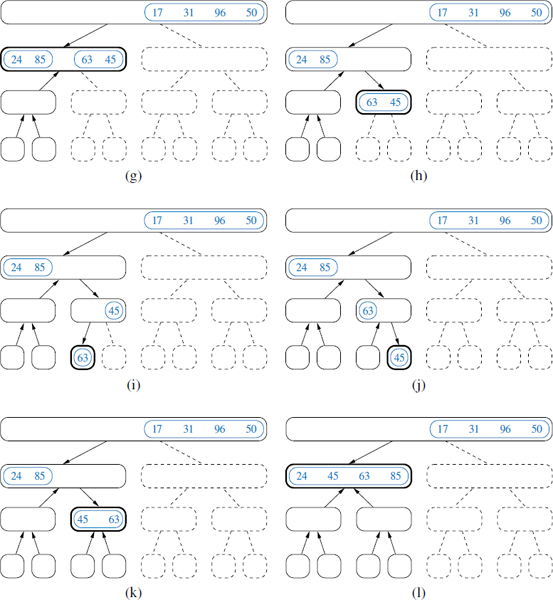
Figure 12.3: Visualization of an execution of merge-sort. (Combined with Figures 12.2 and 12.4.)

Figure 12.4: Visualization of an execution of merge-sort (continued from Figure 12.3). Several calls are omitted between (m) and (n). Note the merging of two halves performed in step (p).

Proposition 12.1: The merge-sort tree associated with an execution of merge-sort on a sequence of size n has height .

We leave the justification of Proposition 12.1 as a simple exercise (R-12.1). We will use this proposition to analyze the running time of the merge-sort algorithm.

Having given an overview of merge-sort and an illustration of how it works, let us consider each of the steps of this divide-and-conquer algorithm in more detail. Dividing a sequence of size n involves separating it at the element with index , and recursive calls can be started by passing these smaller sequences as parameters. The difficult step is combining the two sorted sequences into a single sorted sequence. Thus, before we present our analysis of merge-sort, we need to say more about how this is done.

12.1.2 Array-Based Implementation of Merge-Sort

We begin by focusing on the case when a sequence of items is represented with an array. The merge method (Code Fragment 12.1) is responsible for the subtask of merging two previously sorted sequences, S₁ and S₂, with the output copied into S. We copy one element during each pass of the while loop, conditionally determining whether the next element should be taken from S₁ or S₂. The divide-and-conquer merge-sort algorithm is given in Code Fragment 12.2.

We illustrate a step of the merge process in Figure 12.5. During the process, index i represents the number of elements of _S1 that have been copied to S, while index j represents the number of elements of S₂ that have been copied to S. Assuming S₁ and S₂ both have at least one uncopied element, we copy the smaller of the two elements being considered. Since i + j objects have been previously copied, the next element is placed in S[i + j]. (For example, when i + j is 0, the next element is copied to S[0]). If we reach the end of one of the sequences, we must copy the next element from the other.

Code Fragment 12.1: An implementation of the merge operation for a Java array.

Figure 12.5: A step in the merge of two sorted arrays for which S₂[j] < S₁ [i]. We show the arrays before the copy step in (a) and after it in (b).

Code Fragment 12.2: An implementation of the recursive merge-sort algorithm for a Java array (using the merge method defined in Code Fragment 12.1).

We note that methods merge and mergeSort rely on use of a Comparator instance to compare a pair of generic objects that are presumed to belong to a total order. This is the same approach we introduced when defining priority queues in Section 9.2.2, and when studying implementing sorted maps in Chapters 10 and 11.

12.1.3 The Running Time of Merge-Sort

We begin by analyzing the running time of the merge algorithm. Let n₁ and n₂ be the number of elements of S₁ and S₂, respectively. It is clear that the operations performed inside each pass of the while loop take O(1) time. The key observation is that during each iteration of the loop, one element is copied from either S₁ or S₂ into S (and that element is considered no further). Therefore, the number of iterations of the loop is n₁ + n₂. Thus, the running time of algorithm merge is O(n₁ + n₂).

Having analyzed the running time of the merge algorithm used to combine subproblems, let us analyze the running time of the entire merge-sort algorithm, assuming it is given an input sequence of n elements. For simplicity, we restrict our attention to the case where n is a power of 2. We leave it to an exercise (R-12.3) to show that the result of our analysis also holds when n is not a power of 2.

When evaluating the merge-sort recursion, we rely on the analysis technique introduced in Section 5.2. We account for the amount of time spent within each recursive call, but excluding any time spent waiting for successive recursive calls to terminate. In the case of our mergeSort method, we account for the time to divide the sequence into two subsequences, and the call to merge to combine the two sorted sequences, but we exclude the two recursive calls to mergeSort.

A merge-sort tree T, as portrayed in Figures 12.2 through 12.4, can guide our analysis. Consider a recursive call associated with a node v of the merge-sort tree T. The divide step at node v is straightforward; this step runs in time proportional to the size of the sequence for v, based on the use of slicing to create copies of the two list halves. We have already observed that the merging step also takes time that is linear in the size of the merged sequence. If we let i denote the depth of node v, the time spent at node v is O(n/2ⁱ), since the size of the sequence handled by the recursive call associated with v is equal to n/2ⁱ.

Looking at the tree T more globally, as shown in Figure 12.6, we see that, given our definition of “time spent at a node,” the running time of merge-sort is equal to the sum of the times spent at the nodes of T. Observe that T has exactly 2ⁱ nodes at depth i. This simple observation has an important consequence, for it implies that the overall time spent at all the nodes of T at depth i is O(2ⁱ · n/2ⁱ), which is O(n). By Proposition 12.1, the height of T is . Thus, since the time spent at each of the levels of T is O(n), we have the following result:

Proposition 12.2: Algorithm merge-sort sorts a sequence S of size n in O(n log n) time, assuming two elements of S can be compared in O(1) time.

Figure 12.6: A visual analysis of the running time of merge-sort. Each node represents the time spent in a particular recursive call, labeled with the size of its subproblem.

12.1.4 Merge-Sort and Recurrence Equations

There is another way to justify that the running time of the merge-sort algorithm is O(nlog n) (Proposition 12.2). Namely, we can deal more directly with the recursive nature of the merge-sort algorithm. In this section, we will present such an analysis of the running time of merge-sort, and in so doing, introduce the mathematical concept of a recurrence equation (also known as recurrence relation).

Let the function t (n) denote the worst-case running time of merge-sort on an input sequence of size n. Since merge-sort is recursive, we can characterize function t(n) by means of an equation where the function t(n) is recursively expressed in terms of itself. In order to simplify our characterization of t(n), let us restrict our attention to the case when n is a power of 2. (We leave the problem of showing that our asymptotic characterization still holds in the general case as an exercise.) In this case, we can specify the definition of t(n) as

An expression such as the one above is called a recurrence equation, since the function appears on both the left- and right-hand sides of the equal sign. Although such a characterization is correct and accurate, what we really desire is a big-Oh type of characterization of t(n) that does not involve the function t(n) itself. That is, we want a closed-form characterization of t(n).

We can obtain a closed-form solution by applying the definition of a recurrence equation, assuming n is relatively large. For example, after one more application of the equation above, we can write a new recurrence for t(n) as

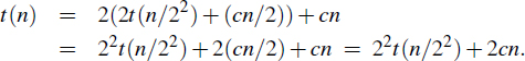
If we apply the equation again, we get t(n) = 2³t(n/2³) + 3cn. At this point, we should see a pattern emerging, so that after applying this equation i times, we get

The issue that remains, then, is to determine when to stop this process. To see when to stop, recall that we switch to the closed form t(n) = b when n ≤ 1, which will occur when 2ⁱ = n. In other words, this will occur when i = log n. Making this substitution, then, yields

That is, we get an alternative justification of the fact that t(n) is O(nlog n).

12.1.5 Alternative Implementations of Merge-Sort

Sorting Linked Lists

The merge-sort algorithm can easily be adapted to use any form of a basic queue as its container type. In Code Fragment 12.3, we provide such an implementation, based on use of the LinkedQueue class from Section 6.2.3. The O(nlogn) bound for merge-sort from Proposition 12.2 applies to this implementation as well, since each basic operation runs in O(1) time when implemented with a linked list. We show an example execution of this version of the merge algorithm in Figure 12.7.

Code Fragment 12.3: An implementation of merge-sort using a basic queue.

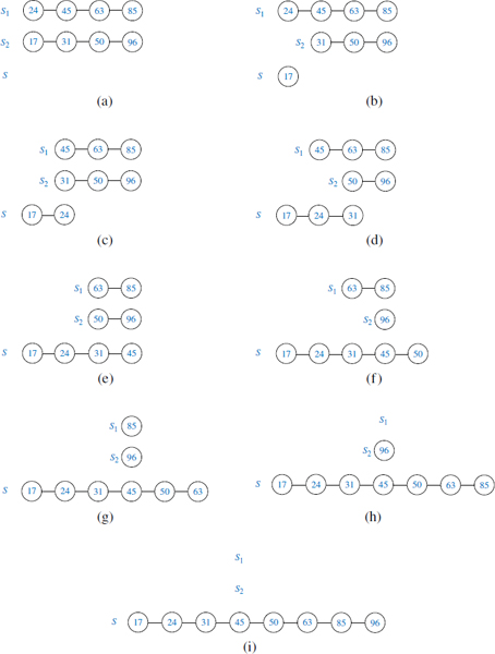
Figure 12.7: Example of an execution of the merge algorithm, as implemented in Code Fragment 12.3 using queues.

A Bottom-Up (Nonrecursive) Merge-Sort

There is a nonrecursive version of array-based merge-sort, which runs in O(nlog n) time. It is a bit faster than recursive merge-sort in practice, as it avoids the extra overheads of recursive calls and temporary memory at each level. The main idea is to perform merge-sort bottom-up, performing the merges level by level going up the merge-sort tree. Given an input array of elements, we begin by merging every successive pair of elements into sorted runs of length two. We merge these runs into runs of length four, merge these new runs into runs of length eight, and so on, until the array is sorted. To keep the space usage reasonable, we deploy a second array that stores the merged runs (swapping input and output arrays after each iteration). We give a Java implementation in Code Fragment 12.4, using the built-in method System.arraycopy to copy arange of cells between two arrays. A similar bottom-up approach can be used for sorting linked lists. (See Exercise C-12.30.)

Code Fragment 12.4: An implementation of the nonrecursive merge-sort algorithm.

12.2 Quick-Sort

The next sorting algorithm we discuss is called quick-sort. Like merge-sort, this algorithm is also based on the divide-and-conquer paradigm, but it uses this technique in a somewhat opposite manner, as all the hard work is done before the recursive calls.

High-Level Description of Quick-Sort

The quick-sort algorithm sorts a sequence S using a simple recursive approach. The main idea is to apply the divide-and-conquer technique, whereby we divide S into subsequences, recur to sort each subsequence, and then combine the sorted subsequences by a simple concatenation. In particular, the quick-sort algorithm consists of the following three steps (see Figure 12.8):

1. Divide: If S has at least two elements (nothing needs to be done if S has zero or one element), select a specific element x from S, which is called the pivot. As is common practice, choose the pivot x to be the last element in S. Remove all the elements from S and put them into three sequences:
   • L, storing the elements in S less than x
   • E, storing the elements in S equal to x
   • G, storing the elements in S greater than x

   Of course, if the elements of S are distinct, then E holds just one element—the pivot itself.

2. Conquer: Recursively sort sequences L and G.
3. Combine: Put back the elements into S in order by first inserting the elements of L, then those of E, and finally those of G.

Figure 12.8: A visual schematic of the quick-sort algorithm.

Like merge-sort, the execution of quick-sort can be visualized by means of a binary recursion tree, called the quick-sort tree. Figure 12.9 summarizes an execution of the quick-sort algorithm by showing the input and output sequences processed at each node of the quick-sort tree. The step-by-step evolution of the quick-sort tree is shown in Figures 12.10, 12.11, and 12.12.

Unlike merge-sort, however, the height of the quick-sort tree associated with an execution of quick-sort is linear in the worst case. This happens, for example, if the sequence consists of n distinct elements and is already sorted. Indeed, in this case, the standard choice of the last element as pivot yields a subsequence L of size n − 1, while subsequence E has size 1 and subsequence G has size 0. At each call of quick-sort on subsequence L, the size decreases by 1. Hence, the height of the quick-sort tree is n − 1.

Figure 12.9: Quick-sort tree T for an execution of the quick-sort algorithm on a sequence with 8 elements: (a) input sequences processed at each node of T; (b) output sequences generated at each node of T. The pivot used at each level of the recursion is shown in bold.

Figure 12.10: Visualization of quick-sort. Each node of the tree represents a recursive call. The nodes drawn with dashed lines represent calls that have not been made yet. The node drawn with thick lines represents the running call. The empty nodes drawn with thin lines represent terminated calls. The remaining nodes represent suspended calls (that is, active calls that are waiting for a child call to return). Note the divide steps performed in (b), (d), and (f). (Continues in Figure 12.11.)

Figure 12.11: Visualization of an execution of quick-sort. Note the concatenation step performed in (k). (Continues in Figure 12.12.)

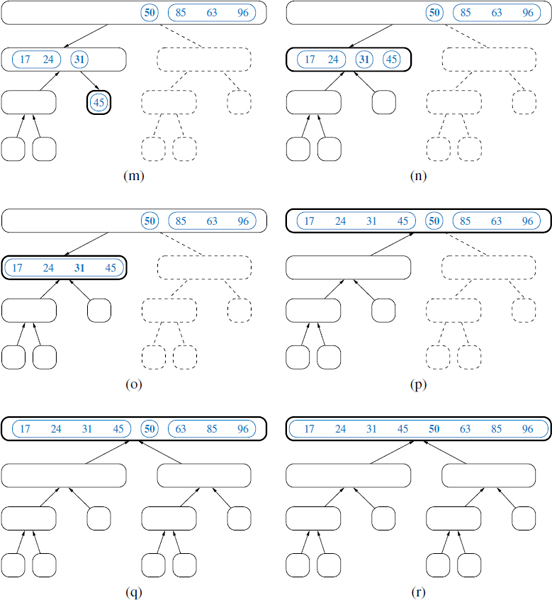
Figure 12.12: Visualization of an execution of quick-sort. Several calls between (p) and (q) have been omitted. Note the concatenation steps performed in (o) and (r). (Continued from Figure 12.11.)

Performing Quick-Sort on General Sequences

In Code Fragment 12.5, we give an implementation of the quick-sort algorithm that works on any sequence type that operates as a queue. This particular version relies on the LinkedQueue class from Section 6.2.3; we provide a more streamlined implementation of quick-sort using an array-based sequence in Section 12.2.2.

Our implementation chooses the first item of the queue as the pivot (since it is easily accessible), and then it divides sequence S into queues L, E, and G of elements that are respectively less than, equal to, and greater than the pivot. We then recur on the L and G lists, and transfer elements from the sorted lists L, E, and G back to S. All of the queue operations run in O(1) worst-case time when implemented with a linked list.

Code Fragment 12.5: Quick-sort for a sequence S implemented as a queue.

Running Time of Quick-Sort

We can analyze the running time of quick-sort with the same technique used for merge-sort in Section 12.1.3. Namely, we can identify the time spent at each node of the quick-sort tree T and sum up the running times for all the nodes.

Examining Code Fragment 12.5, we see that the divide step and the final concatenation of quick-sort can be implemented in linear time. Thus, the time spent at a node v of T is proportional to the input size s(v) of v, defined as the size of the sequence handled by the call of quick-sort associated with node v. Since subsequence E has at least one element (the pivot), the sum of the input sizes of the children of v is at most s(v) − 1.

Let s_i denote the sum of the input sizes of the nodes at depth i for a particular quick-sort tree T. Clearly, s₀ = n, since the root r of T is associated with the entire sequence. Also, s₁ ≤ n − 1, since the pivot is not propagated to the children of r. More generally, it must be that s_i < s_i−1 since the elements of the subsequences at depth i all come from distinct subsequences at depth i − 1, and at least one element from depth i − 1 does not propagate to depth i because it is in a set E (in fact, one element from each node at depth i − 1 does not propagate to depth i).

We can therefore bound the overall running time of an execution of quick-sort as O(n · h) where h is the overall height of the quick-sort tree T for that execution. Unfortunately, in the worst case, the height of a quick-sort tree is n − 1, as observed in Section 12.2. Thus, quick-sort runs in O(n²) worst-case time. Paradoxically, if we choose the pivot as the last element of the sequence, this worst-case behavior occurs for problem instances when sorting should be easy—if the sequence is already sorted.

Given its name, we would expect quick-sort to run quickly, and it often does in practice. The best case for quick-sort on a sequence of distinct elements occurs when subsequences L and G have roughly the same size. In that case, as we saw with merge-sort, the tree has height O(logn) and therefore quick-sort runs in O(nlogn) time; we leave the justification of this fact as an exercise (R-12.12). More so, we can observe an O(nlogn) running time even if the split between L and G is not as perfect. For example, if every divide step caused one subsequence to have one-fourth of those elements and the other to have three-fourths of the elements, the height of the tree would remain O(log n) and thus the overall performance O(n log n).

We will see in the next section that introducing randomization in the choice of a pivot will makes quick-sort essentially behave in this way on average, with an expected running time that is O(n log n).

12.2.1 Randomized Quick-Sort

One common method for analyzing quick-sort is to assume that the pivot will always divide the sequence in a reasonably balanced manner. However, we feel such an assumption would presuppose knowledge about the input distribution that is typically not available. For example, we would have to assume that we will rarely be given “almost” sorted sequences to sort, which are actually common in many applications. Fortunately, this assumption is not needed in order for us to match our intuition to quick-sort's behavior.

In general, we desire some way of getting close to the best-case running time for quick-sort. The way to get close to the best-case running time, of course, is for the pivot to divide the input sequence S almost equally. If this outcome were to occur, then it would result in a running time that is asymptotically the same as the best-case running time. That is, having pivots close to the “middle” of the set of elements leads to an O(nlogn) running time for quick-sort.

Picking Pivots at Random

Since the goal of the partition step of the quick-sort method is to divide the sequence S with sufficient balance, let us introduce randomization into the algorithm and pick as the pivot a random element of the input sequence. That is, instead of picking the pivot as the first or last element of S, we pick an element of S at random as the pivot, keeping the rest of the algorithm unchanged. This variation of quick-sort is called randomized quick-sort. The following proposition shows that the expected running time of randomized quick-sort on a sequence with n elements is O(nlog n). This expectation is taken over all the possible random choices the algorithm makes, and is independent of any assumptions about the distribution of the possible input sequences the algorithm is likely to be given.

Proposition 12.3: The expected running time of randomized quick-sort on a sequence S of size n is O(n log n).

Justification: Let S be a sequence with n elements and let T be the binary tree associated with an execution of randomized quick-sort on S. First, we observe that the running time of the algorithm is proportional to the number of comparisons performed. We consider the recursive call associated with a node of T and observe that during the call, all comparisons are between the pivot element and another element of the input of the call. Thus, we can evaluate the total number of comparisons performed by the algorithm as Σ_s∈SC(x), where C(x) is the number of comparisons involving x as a nonpivot element. Next, we will show that for every element x ∈ S, the expected value of C(x) is O(logn). Since the expected value of a sum is the sum of the expected values of its terms, an O(logn) bound on the expected value of C(x) implies that randomized quick-sort runs in expected O(nlog n) time.

To show that the expected value of C(x) is O(nlogn) for any x, we fix an arbitrary element x and consider the path of nodes in the tree T associated with recursive calls for which x is part of the input sequence. (See Figure 12.13.) By definition, C(x) is equal to that path length, as x will take part in one nonpivot comparison per level of the tree until it is chosen as the pivot or is the only element that remains.

Let n_d denote the input size for the node of that path at depth d of tree T, for 0 ≤ d ≤ C(x). Since all elements are in the initial recursive call, n₀ = n. We know that the input size for any recursive call is at least one less than the size of its parent, and thus that n_d+1 ≤ n_d − 1 for any d < C(x). In the worst case, this implies that C(x) ≤ n − 1, as the recursive process stops if n_d = 1 or if x is chosen as the pivot.

We can show the stronger claim that the expected value of C(x) is O(logn) based on the random selection of a pivot at each level. The choice of pivot at depth d of this path is considered “good” if n_d+1 ≤ 3n_d/4. The choice of a pivot will be good with probability at least 1/2, as there are at least n_d/2 elements in the input that, if chosen as pivot, will result in at least n_d /4 elements begin placed in each subproblem, thereby leaving x in a group with at most 3n_d/4 elements.

We conclude by noting that there can be at most log_4/3n such good pivot choices before x is isolated. Since a choice is good with probability at least 1/2, the expected number of recursive calls before achieving log_4/3 n good choices is at most 2log_4/3 n, which implies that C(x) is O(log n).

With a more rigorous analysis, we can show that the running time of randomized quick-sort is O(nlogn) with high probability. (See Exercise C-12.55.)

Figure 12.13: An illustration of the analysis of Proposition 12.3 for an execution of randomized quick-sort. We focus on element x = 31, which has value C(x) = 3, as it is the nonpivot element in a comparison with 50, 45, and 17. By our notation, n₀ = 10, n₁ = 6, n₂ = 5, and n₃ = 2, and the pivot choices of 50 and 17 are good.

12.2.2 Additional Optimizations for Quick-Sort

An algorithm is in-place if it uses only a small amount of memory in addition to that needed for the original input. Our implementation of heap-sort, from Section 9.4.2, is an example of such an in-place sorting algorithm. Our implementation of quick-sort from Code Fragment 12.5 does not qualify as in-place because we use additional containers L, E, and G when dividing a sequence S within each recursive call. Quick-sort of an array-based sequence can be adapted to be in-place, and such an optimization is used in most deployed implementations.

Performing the quick-sort algorithm in-place requires a bit of ingenuity, however, for we must use the input sequence itself to store the subsequences for all the recursive calls. We show algorithm quickSortInPlace, which performs in-place quick-sort of an array, in Code Fragment 12.6. In-place quick-sort modifies the input sequence using element swapping and does not explicitly create subsequences. Instead, a subsequence of the input sequence is implicitly represented by a range of positions specified by a leftmost index a and a rightmost index b. The divide step is performed by scanning the array simultaneously using local variables left, which advances forward, and right, which advances backward, swapping pairs of elements that are in reverse order, as shown in Figure 12.14. When these two indices pass each other, the division step is complete and the algorithm completes by recurring on these two sublists. There is no explicit “combine” step, because the concatenation of the two sublists is implicit to the in-place use of the original list.

Code Fragment 12.6: In-place quick-sort for an array S. The entire array can be sorted as quickSortInPlace(S, comp, 0, S.length−1).

It is worth noting that if a sequence has duplicate values, we are not explicitly creating three sublists L, E, and G, as in our original quick-sort description. We instead allow elements equal to the pivot (other than the pivot itself) to be dispersed across the two sublists. Exercise R-12.11 explores the subtlety of our implementation in the presence of duplicate keys, and Exercise C-12.34 describes an in-place algorithm that strictly partitions into three sublists L, E, and G.

Figure 12.14: Divide step of in-place quick-sort, using index l as shorthand for identifier left, and index r as shorthand for identifier right. Index l scans the sequence from left to right, and index r scans the sequence from right to left. A swap is performed when l is at an element as large as the pivot and r is at an element as small as the pivot. A final swap with the pivot, in part (f), completes the divide step.

Although the implementation we describe in this section for dividing the sequence into two pieces is in-place, we note that the complete quick-sort algorithm needs space for a stack proportional to the depth of the recursion tree, which in this case can be as large as n − 1. Admittedly, the expected stack depth is O(log n), which is small compared to n. Nevertheless, a simple trick lets us guarantee the stack size is O(log n). The main idea is to design a nonrecursive version of in-place quick-sort using an explicit stack to iteratively process subproblems (each of which can be represented with a pair of indices marking subarray boundaries). Each iteration involves popping the top subproblem, splitting it in two (if it is big enough), and pushing the two new subproblems. The trick is that when pushing the new subproblems, we should first push the larger subproblem and then the smaller one. In this way, the sizes of the subproblems will at least double as we go down the stack; hence, the stack can have depth at most O(log n). We leave the details of this implementation as an exercise (P-12.59).

Pivot Selection

Our implementation in this section blindly picks the last element as the pivot at each level of the quick-sort recursion. This leaves it susceptible to the Θ(n²)-time worst case, most notably when the original sequence is already sorted, reverse sorted, or nearly sorted.

As described in Section 12.2.1, this can be improved upon by using a randomly chosen pivot for each partition step. In practice, another common technique for choosing a pivot is to use the median of tree values, taken respectively from the front, middle, and tail of the array. This median-of-three heuristic will more often choose a good pivot and computing a median of three may require lower overhead than selecting a pivot with a random number generator. For larger data sets, the median of more than three potential pivots might be computed.

Hybrid Approaches

Although quick-sort has very good performance on large data sets, it has rather high overhead on relatively small data sets. For example, the process of quick-sorting a sequence of eight elements, as illustrated in Figures 12.10 through 12.12, involves considerable bookkeeping. In practice, a simple algorithm like insertion-sort (Section 7.6) will execute faster when sorting such a short sequence.

It is therefore common, in optimized sorting implementations, to use a hybrid approach, with a divide-and-conquer algorithm used until the size of a subsequence falls below some threshold (perhaps 50 elements); insertion-sort can be directly invoked upon portions with length below the threshold. We will further discuss such practical considerations in Section 12.4, when comparing the performance of various sorting algorithms.

12.3 Studying Sorting through an Algorithmic Lens

Recapping our discussions on sorting to this point, we have described several methods with either a worst case or expected running time of O(n log n) on an input sequence of size n. These methods include merge-sort and quick-sort, described in this chapter, as well as heap-sort (Section 9.4.2). In this section, we will study sorting as an algorithmic problem, addressing general issues about sorting algorithms.

12.3.1 Lower Bound for Sorting

A natural first question to ask is whether we can sort any faster than O(nlogn) time. Interestingly, if the computational primitive used by a sorting algorithm is the comparison of two elements, this is in fact the best we can do—comparison-based sorting has an Ω(nlog n) worst-case lower bound on its running time. (Recall the notation Ω(·) from Section 4.3.1.) To focus on the main cost of comparison-based sorting, let us only count comparisons, for the sake of a lower bound.

Suppose we are given a sequence S = (x₀, x₁,..., x_n−1) that we wish to sort, and assume that all the elements of S are distinct (this is not really a restriction since we are deriving a lower bound). We do not care if S is implemented as an array or a linked list, for the sake of our lower bound, since we are only counting comparisons. Each time a sorting algorithm compares two elements x_i and x_j (that is, it asks, “is x_i < x_j?”), there are two outcomes: “yes” or “no.” Based on the result of this comparison, the sorting algorithm may perform some internal calculations (which we are not counting here) and will eventually perform another comparison between two other elements of S, which again will have two outcomes. Therefore, we can represent a comparison-based sorting algorithm with a decision tree T (recall Example 8.5). That is, each internal node v in T corresponds to a comparison and the edges from position v to its children correspond to the computations resulting from either a “yes” or “no” answer. It is important to note that the hypothetical sorting algorithm in question probably has no explicit knowledge of the tree T. The tree simply represents all the possible sequences of comparisons that a sorting algorithm might make, starting from the first comparison (associated with the root) and ending with the last comparison (associated with the parent of an external node).

Each possible initial order, or permutation, of the elements in S will cause our hypothetical sorting algorithm to execute a series of comparisons, traversing a path in T from the root to some external node. Let us associate with each external node v in T, then, the set of permutations of S that cause our sorting algorithm to end up in v. The most important observation in our lower-bound argument is that each external node v in T can represent the sequence of comparisons for at most one permutation of S. The justification for this claim is simple: If two different permutations P₁ and P₂ of S are associated with the same external node, then there are at least two objects x_i and x_j, such that x_i is before x_j in P₁ but x_i is after x_j in P₂. At the same time, the output associated with v must be a specific reordering of S, with either x_i or x_j appearing before the other. But if P₁ and P₂ both cause the sorting algorithm to output the elements of S in this order, then that implies there is a way to trick the algorithm into outputting x_i and x_j in the wrong order. Since this cannot be allowed by a correct sorting algorithm, each external node of T must be associated with exactly one permutation of S. We use this property of the decision tree associated with a sorting algorithm to prove the following result:

Proposition 12.4: The running time of any comparison-based algorithm for sorting an n-element sequence is Ω(nlogn) in the worst case.

Justification: The running time of a comparison-based sorting algorithm must be greater than or equal to the height of the decision tree T associated with this algorithm, as described above. (See Figure 12.15.) By the argument above, each external node in T must be associated with one permutation of S. Moreover, each permutation of S must result in a different external node of T. The number of permutations of n objects is n! = n(n − 1)(n − 2)...2 · 1. Thus, T must have at least n! external nodes. By Proposition 8.7, the height of T is at least log(n!). This immediately justifies the proposition, because there are at least n/2 terms that are greater than or equal to n/2 in the product n!; hence,

which is Ω(nlogn).

Figure 12.15: Visualizing the lower bound for comparison-based sorting.

12.3.2 Linear-Time Sorting: Bucket-Sort and Radix-Sort

In the previous section, we showed that Ω(nlog n) time is necessary, in the worst case, to sort an n-element sequence with a comparison-based sorting algorithm. A natural question to ask, then, is whether there are other kinds of sorting algorithms that can be designed to run asymptotically faster than O(nlog n) time. Interestingly, such algorithms exist, but they require special assumptions about the input sequence to be sorted. Even so, such scenarios often arise in practice, such as when sorting integers from a known range or sorting character strings, so discussing them is worthwhile. In this section, we will consider the problem of sorting a sequence of entries, each a key-value pair, where the keys have a restricted type.

Bucket-Sort

Consider a sequence S of n entries whose keys are integers in the range [0, N − 1], for some integer N ≥ 2, and suppose that S should be sorted according to the keys of the entries. In this case, it is possible to sort S in O(n + N) time. It might seem surprising, but this implies, for example, that if N is O(n), then we can sort S in O(n) time. Of course, the crucial point is that, because of the restrictive assumption about the format of the elements, we can avoid using comparisons.

The main idea is to use an algorithm called bucket-sort, which is not based on comparisons, but on using keys as indices into a bucket array B that has cells indexed from 0 to N − 1. An entry with key k is placed in the “bucket” B[k], which itself is a sequence (of entries with key k). After inserting each entry of the input sequence S into its bucket, we can put the entries back into S in sorted order by enumerating the contents of the buckets B[0], B[1],...,B[N − 1] in order. We describe the bucket-sort algorithm in Code Fragment 12.7.

Code Fragment 12.7: Bucket-sort.

It is easy to see that bucket-sort runs in O(n + N) time and uses O(n + N) space. Hence, bucket-sort is efficient when the range N of values for the keys is small compared to the sequence size n, say N = O(n) or N = O(nlogn). Still, its performance deteriorates as N grows compared to n.

An important property of the bucket-sort algorithm is that it works correctly even if there are many different elements with the same key. Indeed, we described it in a way that anticipates such occurrences.

Stable Sorting

When sorting key-value pairs, an important issue is how equal keys are handled. Let S = ((k₀, v₀),..., (k_n−1, v_n−1)) be a sequence of such entries. We say that a sorting algorithm is stable if, for any two entries (k_i, v_i) and (k_j, v_j) of S such that k_i = k_j and (k_i,v_i) precedes (k_j,v_j) in S before sorting (that is, i < j), entry (k_i,v_i) also precedes entry (k_j, v_j) after sorting. Stability is important for a sorting algorithm because applications may want to preserve the initial order of elements with the same key.

Our informal description of bucket-sort in Code Fragment 12.7 guarantees stability as long as we ensure that all sequences act as queues, with elements processed and removed from the front of a sequence and inserted at the back. That is, when initially placing elements of S into buckets, we should process S from front to back, and add each element to the end of its bucket. Subsequently, when transferring elements from the buckets back to S, we should process each B[i] from front to back, with those elements added to the end of S.

Radix-Sort

One of the reasons that stable sorting is so important is that it allows the bucket-sort approach to be applied to more general contexts than to sort integers. Suppose, for example, that we want to sort entries with keys that are pairs (k, l), where k and l are integers in the range [0,N − 1], for some integer N ≥ 2. In a context such as this, it is common to define an order on these keys using the lexicographic (dictionary) convention, where (k₁, l₁) < (k₂, l₂) if k₁ < k₂ or if k₁ = k₂ and l₁ < l₂ (see page 363). This is a pairwise version of the lexicographic comparison function, which can be applied to equal-length character strings, or to tuples of length d.

The radix-sort algorithm sorts a sequence S of entries with keys that are pairs, by applying a stable bucket-sort on the sequence twice; first using one component of the pair as the key when ordering and then using the second component. But which order is correct? Should we first sort on the k's (the first component) and then on the l's (the second component), or should it be the other way around?

To gain intuition before answering this question, we consider the following example.

Example 12.5: Consider the following sequence S (we show only the keys):

If we sort S stably on the first component, then we get the sequence

If we then stably sort this sequence S₁ using the second component, we get the sequence

which is unfortunately not a sorted sequence. On the other hand, if we first stably sort S using the second component, then we get the sequence

If we then stably sort sequence S₂ using the first component, we get the sequence

which is indeed sequence S lexicographically ordered.

So, from this example, we are led to believe that we should first sort using the second component and then again using the first component. This intuition is exactly right. By first stably sorting by the second component and then again by the first component, we guarantee that if two entries are equal in the second sort (by the first component), then their relative order in the starting sequence (which is sorted by the second component) is preserved. Thus, the resulting sequence is guaranteed to be sorted lexicographically every time. We leave to a simple exercise (R-12.19) the determination of how this approach can be extended to triples and other d-tuples of numbers. We can summarize this section as follows:

Proposition 12.6: Let S be a sequence of n key-value pairs, each of which has a key (k₁, k₂,..., k_d), where k_i is an integer in the range [0,N − 1] for some integer N ≥ 2. We can sort S lexicographically in time O(d(n + N)) using radix-sort.

Radix-sort can be applied to any key that can be viewed as a composite of smaller pieces that are to be sorted lexicographically. For example, we can apply it to sort character strings of moderate length, as each individual character can be represented as an integer value. (Some care is needed to properly handle strings with varying lengths.)

12.4 Comparing Sorting Algorithms

At this point, it might be useful for us to take a moment and consider all the algorithms we have studied in this book to sort an n-element sequence.

Considering Running Time and Other Factors

We have studied several methods, such as insertion-sort and selection-sort, that have O(n²)-time behavior in the average and worst case. We have also studied several methods with O(nlog n)-time behavior, including heap-sort, merge-sort, and quick-sort. Finally, the bucket-sort and radix-sort methods run in linear time for certain types of keys. Certainly, the selection-sort algorithm is a poor choice in any application, since it runs in O(n²) time even in the best case. But, of the remaining sorting algorithms, which is the best?

As with many things in life, there is no clear “best” sorting algorithm from the remaining candidates. There are trade-offs involving efficiency, memory usage, and stability. The sorting algorithm best suited for a particular application depends on the properties of that application. In fact, the default sorting algorithm used by computing languages and systems has evolved greatly over time. We can offer some guidance and observations, therefore, based on the known properties of the “good” sorting algorithms.

Insertion-Sort

If implemented well, the running time of insertion-sort is O(n + m), where m is the number of inversions (that is, the number of pairs of elements out of order). Thus, insertion-sort is an excellent algorithm for sorting small sequences (say, less than 50 elements), because insertion-sort is simple to program, and small sequences necessarily have few inversions. Also, insertion-sort is quite effective for sorting sequences that are already “almost” sorted. By “almost,” we mean that the number of inversions is small. But the O(n²)-time performance of insertion-sort makes it a poor choice outside of these special contexts.

Heap-Sort

Heap-sort, on the other hand, runs in O(nlog n) time in the worst case, which is optimal for comparison-based sorting methods. Heap-sort can easily be made to execute in-place, and is a natural choice on small- and medium-sized sequences, when input data can fit into main memory. However, heap-sort tends to be outperformed by both quick-sort and merge-sort on larger sequences. A standard heap-sort does not provide a stable sort, because of the swapping of elements.

Quick-Sort

Although its O(n²)-time worst-case performance makes quick-sort susceptible in real-time applications where we must make guarantees on the time needed to complete a sorting operation, we expect its performance to be O(nlogn) time, and experimental studies have shown that it outperforms both heap-sort and merge-sort on many tests. Quick-sort does not naturally provide a stable sort, due to the swapping of elements during the partitioning step.

For decades quick-sort was the default choice for a general-purpose, in-memory sorting algorithm. Quick-sort was included as the qsort sorting utility provided in C language libraries, and was the basis for sorting utilities on Unix operating systems for many years. It has long been the standard algorithm for sorting arrays of primitive type in Java. (We discuss sorting of object types below.)

Merge-Sort

Merge-sort runs in O(nlogn) time in the worst case. It is quite difficult to make merge-sort run in-place for arrays, and without that optimization the extra overhead of allocate a temporary array, and copying between the arrays is less attractive than in-place implementations of heap-sort and quick-sort for sequences that can fit entirely in a computer's main memory. Even so, merge-sort is an excellent algorithm for situations where the input is stratified across various levels of the computer's memory hierarchy (e.g., cache, main memory, external memory). In these contexts, the way that merge-sort processes runs of data in long merge streams makes the best use of all the data brought as a block into a level of memory, thereby reducing the total number of memory transfers.

The GNU sorting utility (and most current versions of the Linux operating system) relies on a multiway merge-sort variant. Tim-sort (designed by Tim Peters) is a hybrid approach that is essentially a bottom-up merge-sort that takes advantage of initial runs in the data while using insertion-sort to build additional runs. Tim-sort has been the standard sorting algorithm in Python since 2003, and it has become the default algorithm for sorting arrays of object types, as of Java SE 7.

Bucket-Sort and Radix-Sort

Finally, if an application involves sorting entries with small integer keys, character strings, or d-tuples of keys from a discrete range, then bucket-sort or radix-sort is an excellent choice, for it runs in O(d(n+N)) time, where [0,N − 1] is the range of integer keys (and d = 1 for bucket sort). Thus, if d(n + N) is significantly “below” the nlog n function, then this sorting method should run faster than even quick-sort, heap-sort, or merge-sort.

12.5 Selection

As important as it is, sorting is not the only interesting problem dealing with a total order relation on a set of elements. There are a number of applications in which we are interested in identifying a single element in terms of its rank relative to the sorted order of the entire set. Examples include identifying the minimum and maximum elements, but we may also be interested in, say, identifying the median element, that is, the element such that half of the other elements are smaller and the remaining half are larger. In general, queries that ask for an element with a given rank are called order statistics.

Defining the Selection Problem

In this section, we discuss the general order-statistic problem of selecting the k^th smallest element from an unsorted collection of n comparable elements. This is known as the selection problem. Of course, we can solve this problem by sorting the collection and then indexing into the sorted sequence at index k − 1. Using the best comparison-based sorting algorithms, this approach would take O(nlogn) time, which is obviously an overkill for the cases where k = 1 or k = n (or even k = 2, k = 3, k = n − 1, or k = n − 5), because we can easily solve the selection problem for these values of k in O(n) time. Thus, a natural question to ask is whether we can achieve an O(n) running time for all values of k (including the interesting case of finding the median, where ).

12.5.1 Prune-and-Search

We can indeed solve the selection problem in O(n) time for any value of k. Moreover, the technique we use to achieve this result involves an interesting algorithmic design pattern. This design pattern is known as prune-and-search or decrease- and-conquer. In applying this design pattern, we solve a given problem that is defined on a collection of n objects by pruning away a fraction of the n objects and recursively solving the smaller problem. When we have finally reduced the problem to one defined on a constant-sized collection of objects, we then solve the problem using some brute-force method. Returning back from all the recursive calls completes the construction. In some cases, we can avoid using recursion, in which case we simply iterate the prune-and-search reduction step until we can apply a brute-force method and stop. Incidentally, the binary search method described in Section 5.1.3 is an example of the prune-and-search design pattern.

12.5.2 Randomized Quick-Select

In applying the prune-and-search pattern to finding the k^th smallest element in an unordered sequence of n elements, we describe a simple and practical algorithm, known as randomized quick-select. This algorithm runs in O(n) expected time, taken over all possible random choices made by the algorithm; this expectation does not depend whatsoever on any randomness assumptions about the input distribution. We note though that randomized quick-select runs in O(n²) time in the worst case, the justification of which is left as an exercise (R-12.25). We also provide an exercise (C-12.56) for modifying randomized quick-select to define a deterministic selection algorithm that runs in O(n) worst-case time. The existence of this deterministic algorithm is mostly of theoretical interest, however, since the constant factor hidden by the big-Oh notation is relatively large in that case.

Suppose we are given an unsorted sequence S of n comparable elements together with an integer k ∈ [1,n]. At a high level, the quick-select algorithm for finding the k^th smallest element in S is similar to the randomized quick-sort algorithm described in Section 12.2.1. We pick a “pivot” element from S at random and use this to subdivide S into three subsequences L, E, and G, storing the elements of S less than, equal to, and greater than the pivot, respectively. In the prune step, we determine which of these subsets contains the desired element, based on the value of k and the sizes of those subsets. We then recur on the appropriate subset, noting that the desired element's rank in the subset may differ from its rank in the full set. Pseudocode for randomized quick-select is shown in Code Fragment 12.8.

Code Fragment 12.8: Randomized quick-select algorithm.

12.5.3 Analyzing Randomized Quick-Select

Showing that randomized quick-select runs in O(n) time requires a simple probabilistic argument. The argument is based on the linearity of expectation, which states that if X and Y are random variables and c is a number, then

where we use E() to denote the expected value of the expression .

Let t(n) be the running time of randomized quick-select on a sequence of size n. Since this algorithm depends on random events, its running time, t(n), is a random variable. We want to bound E(t(n)), the expected value of t(n). Say that a recursive call of our algorithm is “good” if it partitions S so that the size of each of L and G is at most 3n/4. Clearly, a recursive call is good with probability at least 1/2. Let g(n) denote the number of consecutive recursive calls we make, including the present one, before we get a good one. Then we can characterize t(n) using the following recurrence equation:

where b ≥ 1 is a constant. Applying the linearity of expectation for n > 1, we get

Since a recursive call is good with probability at least 1/2, and whether a recursive call is good or not is independent of its parent call being good, the expected value of g(n) is at most the expected number of times we must flip a fair coin before it comes up “heads.” That is, E(g(n)) ≤ 2. Thus, if we let T(n) be shorthand for E(t(n)), then we can write the case for n > 1 as

To convert this relation into a closed form, let us iteratively apply this inequality assuming n is large. So, for example, after two applications,

At this point, we should see that the general case is

In other words, the expected running time is at most 2bn times a geometric sum whose base is a positive number less than 1. Thus, by Proposition 4.5, T(n) is O(n).

Proposition 12.7: The expected running time of randomized quick-select on a sequence S of size n is O(n), assuming two elements of S can be compared in O(1) time.

12.6 Exercises

Reinforcement

R-12.1	Give a complete justification of Proposition 12.1.
R-12.2	In the merge-sort tree shown in Figures 12.2 through 12.4, some edges are drawn as arrows. What is the meaning of a downward arrow? How about an upward arrow?
R-12.3	Show that the running time of the merge-sort algorithm on an n-element sequence is O(nlogn), even when n is not a power of 2.
R-12.4	Is our array-based implementation of merge-sort given in Section 12.1.2 stable? Explain why or why not.
R-12.5	Is our linked-list-based implementation of merge-sort (Code Fragment 12.3) stable? Explain why or why not.
R-12.6	An algorithm that sorts key-value entries by key is said to be straggling if any time two entries ei and ej have equal keys, but ei appears before ej in the input, then the algorithm places ei after ej in the output. Describe a change to the merge-sort algorithm in Section 12.1 to make it straggling.
R-12.7	Suppose we are given two n-element sorted sequences A and B each with distinct elements, but potentially some elements that are in both sequences. Describe an O(n)-time method for computing a sequence representing the union A ∪ B (with no duplicates) as a sorted sequence.
R-12.8	Give pseudocode descriptions for the retainAll and removeAll methods of the set ADT, assuming we use sorted sequences to implement sets.
R-12.9	Suppose we modify the deterministic version of the quick-sort algorithm so that, instead of selecting the last element in an n-element sequence as the pivot, we choose the element at index . What is the running time of this version of quick-sort on a sequence that is already sorted?
R-12.10	Consider a modification of the deterministic version of the quick-sort algorithm where we choose the element at index as our pivot. Describe the kind of sequence that would cause this version of quick-sort to run in Ω(n2) time.
R-12.11	Suppose the method quickSortInPlace is executed on a sequence with duplicate elements. Prove that the algorithm still correctly sorts the input sequence. What happens in the partition step when there are elements equal to the pivot? What is the running time of the algorithm if all the input elements are equal?
R-12.12	Show that the best-case running time of quick-sort on a sequence of size n with distinct elements is Ω(nlogn).
R-12.13	If the outermost while loop of our implementation of quickSortInPlace (line 9 of Code Fragment 12.6) were changed to use condition left < right, instead of condition left <= right, there would be a flaw. Explain the flaw and give a specific input sequence on which such an implementation fails.
R-12.14	If the conditional at line 14 of our quickSortInPlace implementation of Code Fragment 12.6 were changed to use condition left < right, instead of condition left <= right, there would be a flaw. Explain the flaw and give a specific input sequence on which such an implementation fails.
R-12.15	Following our analysis of randomized quick-sort in Section 12.2.1, show that the probability that a given input element x belongs to more than 2 log n subproblems in size group i is at most 1/n2.
R-12.16	Of the n! possible inputs to a given comparison-based sorting algorithm, what is the absolute maximum number of inputs that could be correctly sorted with just n comparisons?
R-12.17	Jonathan has a comparison-based sorting algorithm that sorts the first k elements of a sequence of size n in O(n) time. Give a big-Oh characterization of the biggest that k can be.
R-12.18	Is the bucket-sort algorithm in-place? Why or why not?
R-12.19	Describe a radix-sort method for lexicographically sorting a sequence S of triplets (k, l, m), where k, l, and m are integers in the range [0,N − 1], for N ≥ 2. How could this scheme be extended to sequences of d-tuples (k1,k2,...,kd), where each ki is an integer in the range [0,N − 1]?
R-12.20	Suppose S is a sequence of n values, each equal to 0 or 1. How long will it take to sort S with the merge-sort algorithm? What about quick-sort?
R-12.21	Suppose S is a sequence of n values, each equal to 0 or 1. How long will it take to sort S stably with the bucket-sort algorithm?
R-12.22	Given a sequence S of n values, each equal to 0 or 1, describe an in-place method for sorting S.
R-12.23	Give an example input that requires merge-sort and heap-sort to take O(nlogn) time to sort, but insertion-sort runs in O(n) time. What if you reverse this list?
R-12.24	What is the best algorithm for sorting each of the following: general comparable objects, long character strings, 32-bit integers, double-precision floating-point numbers, and bytes? Justify your answer.
R-12.25	Show that the worst-case running time of quick-select on an n-element sequence is Ω(n2).

Creativity

C-12.26	Describe and analyze an efficient method for removing all duplicates from a collection A of n elements.
C-12.27	Augment the PositionalList class (see Section 7.3) to support a method named sort that sorts the elements of a list by relinking existing nodes; you are not to create any new nodes. You may use your choice of sorting algorithm.
C-12.28	Linda claims to have an algorithm that takes an input sequence S and produces an output sequence T that is a sorting of the n elements in S. Give an algorithm, isSorted, that tests in O(n) time if T is sorted. Explain why the algorithm isSorted is not sufficient to prove a particular output T to Linda's algorithm is a sorting of S. Describe what additional information Linda's algorithm could output so that her algorithm's correctness could be established on any given S and T in O(n) time.
C-12.29	Augment the PositionalList class (see Section 7.3) to support a method named merge with the following behavior. If A and B are PositionalList instances whose elements are sorted, the syntax A.merge(B) should merge all elements of B into A so that A remains sorted and B becomes empty. Your implementation must accomplish the merge by relinking existing nodes; you are not to create any new nodes.
C-12.30	Implement a bottom-up merge-sort for a collection of items by placing each item in its own queue, and then repeatedly merging pairs of queues until all items are sorted within a single queue.
C-12.31	Modify our in-place quick-sort implementation of Code Fragment 12.6 to be a randomized version of the algorithm, as discussed in Section 12.2.1.
C-12.32	Consider a version of deterministic quick-sort where we pick as our pivot the median of the d last elements in the input sequence of n elements, for a fixed, constant odd number d ≥ 3. What is the asymptotic worst-case running time of quick-sort in this case?
C-12.33	Another way to analyze randomized quick-sort is to use a recurrence equation. In this case, we let T(n) denote the expected running time of randomized quicksort, and we observe that, because of the worst-case partitions for good and bad splits, we can write where bn is the time needed to partition a list for a given pivot and concatenate the result sublists after the recursive calls return. Show, by induction, that T(n) is O(nlogn).
C-12.34	Our high-level description of quick-sort describes partitioning the elements into three sets L, E, and G, having keys less than, equal to, or greater than the pivot, respectively. However, our in-place quick-sort implementation of Code Fragment 12.6 does not gather all elements equal to the pivot into a set E. An alternative strategy for an in-place, three-way partition is as follows. Loop through the elements from left to right maintaining indices a, b, and c and the invariant that elements with index i such that 0 ≤ i < a are strictly less than the pivot, those with a ≤ i < b are equal to the pivot, and those with index b ≤ i < c are strictly greater than the pivot; elements with index c ≤ i < n are yet unclassified. In each pass of the loop, classify one additional element, performing a constant number of swaps as needed. Implement an in-place quick-sort using this strategy.
C-12.35	Suppose we are given an n-element sequence S such that each element in S represents a different vote for president, where each vote is given as an integer representing a particular candidate, yet the integers may be arbitrarily large (even if the number of candidates is not). Design an O(nlogn)-time algorithm to see who wins the election S represents, assuming the candidate with the most votes wins.
C-12.36	Consider the voting problem from Exercise C-12.35, but now suppose that we know the number k < n of candidates running, even though the integer IDs for those candidates can be arbitrarily large. Describe an O(nlogk)-time algorithm for determining who wins the election.
C-12.37	Consider the voting problem from Exercise C-12.35, but now suppose the integers 1 to k are used to identify k < n candidates. Design an O(n)-time algorithm to determine who wins the election.
C-12.38	Show that any comparison-based sorting algorithm can be made to be stable without affecting its asymptotic running time.
C-12.39	Suppose we are given two sequences A and B of n elements, possibly containing duplicates, on which a total order relation is defined. Describe an efficient algorithm for determining if A and B contain the same set of elements. What is the running time of this method?
C-12.40	Given an array A of n integers in the range [0,n2 − 1], describe a simple method for sorting A in O(n) time.
C-12.41	Let S1, S2,..., Sk be k different sequences whose elements have integer keys in the range [0,N − 1], for some parameter N ≥ 2. Describe an algorithm that produces k respective sorted sequences in O(n + N) time, where n denotes the sum of the sizes of those sequences.
C-12.42	Given a sequence S of n elements, on which a total order relation is defined, describe an efficient method for determining whether there are two equal elements in S. What is the running time of your method?
C-12.43	Let S be a sequence of n elements on which a total order relation is defined. Recall that an inversion in S is a pair of elements x and y such that x appears before y in S but x > y. Describe an algorithm running in O(nlogn) time for determining the number of inversions in S.
C-12.44	Let S be a sequence of n integers. Describe a method for printing out all the pairs of inversions in S in O(n + k) time, where k is the number of such inversions.
C-12.45	Let S be a random permutation of n distinct integers. Argue that the expected running time of insertion-sort on S is Ω (n2). (Hint: Note that half of the elements ranked in the top half of a sorted version of S are expected to be in the first half of S.)
C-12.46	Let A and B be two sequences of n integers each. Given an integer m, describe an O(nlogn)-time algorithm for determining if there is an integer a in A and an integer b in B such that m = a + b.
C-12.47	Given two sets A and B represented as sorted sequences, describe an efficient algorithm for computing A ⊕ B, which is the set of elements that are in A or B, but not in both.
C-12.48	Given a set of n integers, describe and analyze a fast method for finding the integers closest to the median.
C-12.49	Bob has a set A of n nuts and a set B of n bolts, such that each nut in A has a unique matching bolt in B. Unfortunately, the nuts in A all look the same, and the bolts in B all look the same as well. The only kind of a comparison that Bob can make is to take a nut-bolt pair (a, b), such that a is in A and b is in B, and test it to see if the threads of a are larger, smaller, or a perfect match with the threads of b. Describe and analyze an efficient algorithm for Bob to match up all of his nuts and bolts.
C-12.50	Our quick-select implementation can be made more space-efficient by initially computing only the counts for sets L, E, and G, and creating only the new subset that will be needed for recursion. Implement such a version.
C-12.51	Describe an in-place version of the quick-select algorithm in pseudocode, assuming that you are allowed to modify the order of elements.
C-12.52	Show how to use a deterministic O(n)-time selection algorithm to sort a sequence of n elements in O(nlogn)-worst-case time.
C-12.53	Given an unsorted sequence S of n comparable elements, and an integer k, give an O(nlogk)-expected-time algorithm for finding the O(k) elements that have rank , , , and so on.
C-12.54	Space aliens have given us a method, alienSplit, that can take a sequence S of n integers and partition S in O(n) time into sequences S1, S2,..., Sk of size at most each, such that the elements in Si are less than or equal to every element in Si+1, for i = 1,2,..., k − 1, for a fixed number, k < n. Show how to use alienSplit to sort S in O(nlogn/logk) time.
C-12.55	Show that randomized quick-sort runs in O(n log n) time with probability at least 1 − 1/n, that is, with high probability, by answering the following: For each input element x, define Ci,j(x) to be a 0/1 random variable that is 1 if and only if element x is in j + 1 subproblems that have size s such that (3/4)i+1n < s ≤ (3/4)in. Argue why we need not define Ci,j for j > n. Let Xi,j be an independent 0/1 random variable that is 1 with probability 1/2j, and let . Argue that . Show that the expected value of is (2 − 1/2n)L. Show that the probability that is at most 1/n2, using the Chernoff bound that states that if X is the sum of a finite number of independent 0/1 random variables, having expected value μ > 0, then Pr(X > 2μ) < (4/e)−μ, where e = 2.71828128.... Argue that randomized quick-sort runs in O(nlogn) time with probability at least 1 − 1/n.
C-12.56	We can make the quick-select algorithm deterministic, by choosing the pivot of an n-element sequence as follows: Partition the set S into groups of size 5 each (except possibly for one group). Sort each little set and identify the median element in this set. From this set of “baby” medians, apply the selection algorithm recursively to find the median of the baby medians. Use this element as the pivot and proceed as in the quick-select algorithm. Show that this deterministic quick-select algorithm runs in O(n) time by answering the following questions (please ignore floor and ceiling functions if that simplifies the mathematics, for the asymptotics are the same either way): How many baby medians are less than or equal to the chosen pivot? How many are greater than or equal to the pivot? For each baby median less than or equal to the pivot, how many other elements are less than or equal to the pivot? Is the same true for those greater than or equal to the pivot? Argue why the method for finding the deterministic pivot and using it to partition S takes O(n) time. Based on these estimates, write a recurrence equation to bound the worst-case running time t(n) for this selection algorithm (note that in the worst case there are two recursive calls—one to find the median of the baby medians and one to recur on the larger of L and G). Using this recurrence equation, show by induction that t(n) is O(n).
C-12.57	Suppose we are interested in dynamically maintaining a set S of integers, which is initially empty, while supporting the following two operations: add(v): Adds value v to set S. median(): Returns the current median value of the set. For a set with even cardinality, we define the median as the average of the two most central values. We will store each element of the set in one of two priority queues: a min-oriented priority queue, Q+, of all elements greater than or equal to the current median value, and a max-oriented priority queue, Q−, of all elements less than the current median value. Explain how to perform the operation median() in O(1) time given such a representation. Explain how to perform the operation S.add(k) in O(log n) time, where n is the current cardinality of the set, while maintaining such a representation.
C-12.58	As a generalization of the previous problem, revisit Exercise C-11.45, which involves performing general selection queries on a dynamic set of values.

Projects

P-12.59	Implement a nonrecursive, in-place version of the quick-sort algorithm, as described at the end of Section 12.2.2.
P-12.60	Experimentally compare the performance of in-place quick-sort and a version of quick-sort that is not in-place.
P-12.61	Perform a series of benchmarking tests on a version of merge-sort and quick-sort to determine which one is faster. Your tests should include sequences that are “random” as well as “almost” sorted.
P-12.62	Implement deterministic and randomized versions of the quick-sort algorithm and perform a series of benchmarking tests to see which one is faster. Your tests should include sequences that are very “random” looking as well as ones that are “almost” sorted.
P-12.63	Implement an in-place version of insertion-sort and an in-place version of quicksort. Perform benchmarking tests to determine the range of values of n where quick-sort is on average better than insertion-sort.
P-12.64	Design and implement a version of the bucket-sort algorithm for sorting a list of n entries with integer keys taken from the range [0,N − 1], for N ≥ 2. The algorithm should run in O(n + N) time.
P-12.65	Implement an animation of one of the sorting algorithms described in this chapter, illustrating key properties of the algorithm in an intuitive manner.
P-12.66	Design and implement two versions of the bucket-sort algorithm in Java, one for sorting an array of byte values and one for sorting an array of short values. Experimentally compare the performance of your implementations with that of the method, java.util.Arrays.sort.

Chapter Notes

Knuth's classic text on Sorting and Searching [61] contains an extensive history of the sorting problem and algorithms for solving it. Huang and Langston [49] show how to merge two sorted lists in-place in linear time. The standard quick-sort algorithm is due to Hoare [45]. Several optimizations for quick-sort are described by Bentley and McIlroy [15]. More information about randomized algorithms can be found in the book by Motwani and Raghavan [75]. The quick-sort analysis given in this chapter is a combination of the analysis given in an earlier Java edition of this book and the analysis of Kleinberg and Tardos [57]. Exercise C-12.33 is due to Littman. Gonnet and Baeza-Yates [38] analyze and compare experimentally several sorting algorithms. The term “prune-and-search” comes originally from the computational geometry literature (such as in the work of Clarkson [22] and Megiddo [70]). The term “decrease-and-conquer” is from Levitin [66].