Chapter
9

Priority Queues

Contents

9.1 The Priority Queue Abstract Data Type

9.1.1 Priorities

In Chapter 6, we introduced the queue ADT as a collection of objects that are added and removed according to the first-in, first-out (FIFO) principle. A company's customer call center embodies such a model in which waiting customers are told “calls will be answered in the order that they were received.” In that setting, a new call is added to the back of the queue, and each time a customer service representative becomes available, he or she is connected with the call that is removed from the front of the call queue.

In practice, there are many applications in which a queue-like structure is used to manage objects that must be processed in some way, but for which the first-in, first-out policy does not suffice. Consider, for example, an air-traffic control center that has to decide which flight to clear for landing from among many approaching the airport. This choice may be influenced by factors such as each plane's distance from the runway, time spent waiting in a holding pattern, or amount of remaining fuel. It is unlikely that the landing decisions are based purely on a FIFO policy.

There are other situations in which a “first come, first serve” policy might seem reasonable, yet for which other priorities come into play. To use another airline analogy, suppose a certain flight is fully booked an hour prior to departure. Because of the possibility of cancellations, the airline maintains a queue of standby passengers hoping to get a seat. Although the priority of a standby passenger is influenced by the check-in time of that passenger, other considerations include the fare paid and frequent-flyer status. So it may be that an available seat is given to a passenger who has arrived later than another, if such a passenger is assigned a better priority by the airline agent.

In this chapter, we introduce a new abstract data type known as a priority queue. This is a collection of prioritized elements that allows arbitrary element insertion, and allows the removal of the element that has first priority. When an element is added to a priority queue, the user designates its priority by providing an associated key. The element with the minimal key will be the next to be removed from the queue (thus, an element with key 1 will be given priority over an element with key 2). Although it is quite common for priorities to be expressed numerically, any Java object may be used as a key, as long as there exists means to compare any two instances a and b, in a way that defines a natural order of the keys. With such generality, applications may develop their own notion of priority for each element. For example, different financial analysts may assign different ratings (i.e., priorities) to a particular asset, such as a share of stock.

9.1.2 The Priority Queue ADT

We model an element and its priority as a key-value composite known as an entry. (However, we defer until Section 9.2.1 the technical definition of the Entry type.)

We define the priority queue ADT to support the following methods:

insert(k, v):	Creates an entry with key k and value v in the priority queue.
min():	Returns (but does not remove) a priority queue entry (k,v) having minimal key; returns null if the priority queue is empty.
removeMin():	Removes and returns an entry (k,v) having minimal key from the priority queue; returns null if the priority queue is empty.
size():	Returns the number of entries in the priority queue.
isEmpty():	Returns a boolean indicating whether the priority queue is empty.

A priority queue may have multiple entries with equivalent keys, in which case methods min and removeMin may report an arbitrary choice among those entry having minimal key. Values may be any type of object.

In our initial model for a priority queue, we assume that an element's key remains fixed once it has been added to a priority queue. In Section 9.5, we consider an extension that allows a user to update an element's key within the priority queue.

Example 9.1: The following table shows a series of operations and their effects on an initially empty priority queue. The “Priority Queue Contents” column is somewhat deceiving since it shows the entries sorted by key. Such an internal representation is not required of a priority queue.

9.2 Implementing a Priority Queue

In this section, we discuss several technical issues involving the implementation of the priority queue ADT in Java, and we define an abstract base class that provides functionality that is shared by all priority queue implementations in this chapter. We then provide two concrete priority queue implementations using a positional list L (see Section 7.3) for storage. They differ in whether or not entries are maintained in sorted order according to their keys.

9.2.1 The Entry Composite

One challenge in implementing a priority queue is that we must keep track of both an element and its key, even as entries are relocated within a data structure. This is reminiscent of a case study from Section 7.7 in which we maintain a list of elements with access frequencies. In that setting, we introduced the composition design pattern, defining an Item class that paired each element with its associated count in our primary data structure. For priority queues, we use composition to pair a key k and a value v as a single object. To formalize this, we define the public interface, Entry, shown in Code Fragment 9.1.

Code Fragment 9.1: Java interface for an entry storing a key-value pair.

We then use the Entry type in the formal interface for the priority queue, shown in Code Fragment 9.2. This allows us to return both a key and value as a single object from methods such as min and removeMin. We also define the insert method to return an entry; in a more advanced adaptable priority queue (see Section 9.5), that entry can be subsequently updated or removed.

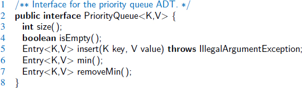
Code Fragment 9.2: Java interface for the priority queue ADT.

9.2.2 Comparing Keys with Total Orders

In defining the priority queue ADT, we can allow any type of object to serve as a key, but we must be able to compare keys to each other in a meaningful way. More so, the results of the comparisons must not be contradictory. For a comparison rule, which we denote by ≤, to be self-consistent, it must define a total order relation, which is to say that it satisfies the following properties for any keys k₁, k₂, and k₃:

• Comparability property: k₁ ≤ k₂ or k₂ ≤ k₁.
• Antisymmetric property: if k₁ ≤ k₂ and k₂ ≤ k₁, then k₁ = k₂.
• Transitive property: if k₁ ≤ k₂ and k₂ ≤ k₃, then k₁ ≤ k₃.

The comparability property states that comparison rule is defined for every pair of keys. Note that this property implies the following one:

• Reflexive property: k ≤ k.

A comparison rule, ≤, that defines a total order relation will never lead to a contradiction. Such a rule defines a linear ordering among a set of keys; hence, if a (finite) set of elements has a total order defined for it, then the notion of a minimal key, k_min, is well defined, as a key in which k_min ≤ k, for any other key k in our set.

The Comparable Interface

Java provides two means for defining comparisons between object types. The first of these is that a class may define what is known as the natural ordering of its instances by formally implementing the java.lang.Comparable interface, which includes a single method, compareTo. The syntax a.compareTo(b) must return an integer i with the following meaning:

• i < 0 designates that a < b.
• i = 0 designates that a = b.
• i > 0 designates that a > b.

For example, the compareTo method of the String class defines the natural ordering of strings to be lexicographic, which is a case-sensitive extension of the alphabetic ordering to Unicode.

The Comparator Interface

In some applications, we may want to compare objects according to some notion other than their natural ordering. For example, we might be interested in which of two strings is the shortest, or in defining our own complex rules for judging which of two stocks is more promising. To support generality, Java defines the java.util.Comparator interface. A comparator is an object that is external to the class of the keys it compares. It provides a method with the signature compare(a, b) that returns an integer with similar meaning to the compareTo method described above.

As a concrete example, Code Fragment 9.3 defines a comparator that evaluates strings based on their length (rather than their natural lexicographic order).

Code Fragment 9.3: A comparator that evaluates strings based on their lengths.

Comparators and the Priority Queue ADT

For a general and reusable form of a priority queue, we allow a user to choose any key type and to send an appropriate comparator instance as a parameter to the priority queue constructor. The priority queue will use that comparator anytime it needs to compare two keys to each other.

For convenience, we also allow a default priority queue to instead rely on the natural ordering for the given keys (assuming those keys come from a comparable class). In that case, we build our own instance of a Default Comparator class, shown in Code Fragment 9.4.

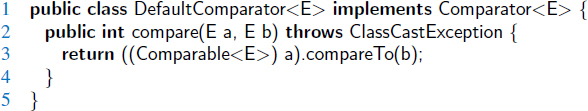
Code Fragment 9.4: A DefaultComparator class that implements a comparator based upon the natural ordering of its element type.

9.2.3 The AbstractPriorityQueue Base Class

To manage technical issues common to all our priority queue implementations, we define an abstract base class named AbstractPriorityQueue in Code Fragment 9.5. (See Section 2.3.3 for a discussion of abstract base classes.) This includes a nested PQEntry class that implements the public Entry interface.

Our abstract class also declares and initializes an instance variable, comp, that stores the comparator being used for the priority queue. We then provide a protected method, compare, that invokes the comparator on the keys of two given entries.

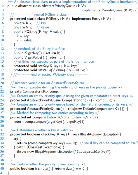
Code Fragment 9.5: The AbstractPriorityQueue class. This provides a nested PQEntry class that composes a key and a value into a single object, and support for managing a comparator. For convenience, we also provide an implementation of isEmpty based on a presumed size method.

9.2.4 Implementing a Priority Queue with an Unsorted List

In our first concrete implementation of a priority queue, we store entries within an unsorted linked list. Code Fragment 9.6 presents our UnsortedPriorityQueue class as a subclass of the AbstractPriorityQueue class (from Code Fragment 9.5). For internal storage, key-value pairs are represented as composites, using instances of the inherited PQEntry class. These entries are stored within a PositionalList that is an instance variable. We assume that the positional list is implemented with a doubly linked list, as in Section 7.3, so that all operations of that ADT execute in O(1) time.

We begin with an empty list when a new priority queue is constructed. At all times, the size of the list equals the number of key-value pairs currently stored in the priority queue. For this reason, our priority queue size method simply returns the length of the internal list. By the design of our AbstractPriorityQueue class, we inherit a concrete implementation of the isEmpty method that relies on a call to our size method.

Each time a key-value pair is added to the priority queue, via the insert method, we create a new PQEntry composite for the given key and value, and add that entry to the end of the list. Such an implementation takes O(1) time.

The remaining challenge is that when min or removeMin is called, we must locate the entry with minimal key. Because the entries are not sorted, we must inspect all entries to find one with a minimal key. For convenience, we define a private findMin utility that returns the position of an entry with minimal key. Knowledge of the position allows the removeMin method to invoke the remove method on the positional list. The min method simply uses the position to retrieve the entry when preparing a key-value tuple to return. Due to the loop for finding the minimal key, both min and removeMin methods run in O(n) time, where n is the number of entries in the priority queue.

A summary of the running times for the UnsortedPriorityQueue class is given in Table 9.1.

Method	Running Time
size	O(1)
isEmpty	O(1)
insert	O(1)
min	O(n)
removeMin	O(n)

Table 9.1: Worst-case running times of the methods of a priority queue of size n, realized by means of an unsorted, doubly linked list. The space requirement is O(n).

Code Fragment 9.6: An implementation of a priority queue using an unsorted list. The parent class AbstractPriorityQueue is given in Code Fragment 9.5, and the LinkedPositionalList class is from Section 7.3.

9.2.5 Implementing a Priority Queue with a Sorted List

Our next implementation of a priority queue also uses a positional list, yet maintains entries sorted by nondecreasing keys. This ensures that the first element of the list is an entry with the smallest key.

Our SortedPriorityQueue class is given in Code Fragment 9.7. The implementation of min and removeMin are rather straightforward given knowledge that the first element of a list has a minimal key. We rely on the first method of the positional list to find the position of the first entry, and the remove method to remove the entry from the list. Assuming that the list is implemented with a doubly linked list, operations min and removeMin take O(1) time.

This benefit comes at a cost, however, for method insert now requires that we scan the list to find the appropriate position to insert the new entry. Our implementation starts at the end of the list, walking backward until the new key is smaller than that of an existing entry; in the worst case, it progresses until reaching the front of the list. Therefore, the insert method takes O(n) worst-case time, where n is the number of entries in the priority queue at the time the method is executed. In summary, when using a sorted list to implement a priority queue, insertion runs in linear time, whereas finding and removing the minimum can be done in constant time.

Comparing the Two List-Based Implementations

Table 9.2 compares the running times of the methods of a priority queue realized by means of a sorted and unsorted list, respectively. We see an interesting tradeoff when we use a list to implement the priority queue ADT. An unsorted list supports fast insertions but slow queries and deletions, whereas a sorted list allows fast queries and deletions, but slow insertions.

Table 9.2: Worst-case running times of the methods of a priority queue of size n, realized by means of an unsorted or sorted list, respectively. We assume that the list is implemented by a doubly linked list. The space requirement is O(n).

Code Fragment 9.7: An implementation of a priority queue using a sorted list. The parent class AbstractPriorityQueue is given in Code Fragment 9.5, and the LinkedPositionalList class is from Section 7.3.

9.3 Heaps

The two strategies for implementing a priority queue ADT in the previous section demonstrate an interesting trade-off. When using an unsorted list to store entries, we can perform insertions in O(1) time, but finding or removing an element with minimal key requires an O(n)-time loop through the entire collection. In contrast, if using a sorted list, we can trivially find or remove the minimal element in O(1) time, but adding a new element to the queue may require O(n) time to restore the sorted order.

In this section, we provide a more efficient realization of a priority queue using a data structure called a binary heap. This data structure allows us to perform both insertions and removals in logarithmic time, which is a significant improvement over the list-based implementations discussed in Section 9.2. The fundamental way the heap achieves this improvement is to use the structure of a binary tree to find a compromise between elements being entirely unsorted and perfectly sorted.

9.3.1 The Heap Data Structure

A heap (see Figure 9.1) is a binary tree T that stores entries at its positions, and that satisfies two additional properties: a relational property defined in terms of the way keys are stored in T and a structural property defined in terms of the shape of T itself. The relational property is the following:

Heap-Order Property: In a heap T, for every position p other than the root, the key stored at p is greater than or equal to the key stored at p's parent.

As a consequence of the heap-order property, the keys encountered on a path from the root to a leaf of T are in nondecreasing order. Also, a minimal key is always stored at the root of T. This makes it easy to locate such an entry when min or removeMin is called, as it is informally said to be “at the top of the heap” (hence, the name “heap” for the data structure). By the way, the heap data structure defined here has nothing to do with the memory heap (Section 15.1.2) used in the runtime environment supporting a programming language like Java.

For the sake of efficiency, as will become clear later, we want the heap T to have as small a height as possible. We enforce this requirement by insisting that the heap T satisfy an additional structural property; it must be what we term complete.

Complete Binary Tree Property: A heap T with height h is a complete binary tree if levels 0,1,2, ...,h−1 of T have the maximal number of nodes possible (namely, level i has 2ⁱ nodes, for 0 ≤ i ≤ h−1) and the remaining nodes at level h reside in the leftmost possible positions at that level.

Figure 9.1: Example of a heap storing 13 entries with integer keys. The last position is the one storing entry (13, W).

The tree in Figure 9.1 is complete because levels 0, 1, and 2 are full, and the six nodes in level 3 are in the six leftmost possible positions at that level. In formalizing what we mean by the leftmost possible positions, we refer to the discussion of level numbering from Section 8.3.2, in the context of an array-based representation of a binary tree. (In fact, in Section 9.3.2 we will discuss the use of an array to represent a heap.) A complete binary tree with n elements is one that has positions with level numbering 0 through n−1. For example, in an array-based representation of the above tree, its 13 entries would be stored consecutively from A[0] to A[12].

The Height of a Heap

Let h denote the height of T. Insisting that T be complete also has an important consequence, as shown in Proposition 9.2.

Proposition 9.2: A heap T storing n entries has height .

Justification: From the fact that T is complete, we know that the number of nodes in levels 0 through h−1 of T is precisely 1+2+4+···+2^h−1 = 2h−1, and that the number of nodes in level h is at least 1 and at most 2^h. Therefore

By taking the logarithm of both sides of inequality n ≥ 2^h, we see that height h ≤ log n. By rearranging terms and taking the logarithm of both sides of inequality n ≤ 2^{h + 1} −1, we see that h ≥ log(n + 1)− 1. Since h is an integer, these two inequalities imply that .

9.3.2 Implementing a Priority Queue with a Heap

Proposition 9.2 has an important consequence, for it implies that if we can perform update operations on a heap in time proportional to its height, then those operations will run in logarithmic time. Let us therefore turn to the problem of how to efficiently perform various priority queue methods using a heap.

We will use the composition pattern from Section 9.2.1 to store key-value pairs as entries in the heap. The size and isEmpty methods can be implemented based on examination of the tree, and the min operation is equally trivial because the heap property assures that the element at the root of the tree has a minimal key. The interesting algorithms are those for implementing the insert and removeMin methods.

Adding an Entry to the Heap

Let us consider how to perform insert(k, v) on a priority queue implemented with a heap T. We store the pair (k, v) as an entry at a new node of the tree. To maintain the complete binary tree property, that new node should be placed at a position p just beyond the rightmost node at the bottom level of the tree, or as the leftmost position of a new level, if the bottom level is already full (or if the heap is empty).

Up-Heap Bubbling After an Insertion

After this action, the tree T is complete, but it may violate the heap-order property. Hence, unless position p is the root of T (that is, the priority queue was empty before the insertion), we compare the key at position p to that of p's parent, which we denote as q. If key k_p ≥ k_q, the heap-order property is satisfied and the algorithm terminates. If instead k_p < k_q, then we need to restore the heap-order property, which can be locally achieved by swapping the entries stored at positions p and q. (See Figure 9.2c and d.) This swap causes the new entry to move up one level. Again, the heap-order property may be violated, so we repeat the process, going up in T until no violation of the heap-order property occurs. (See Figure 9.2e and h.)

The upward movement of the newly inserted entry by means of swaps is conventionally called up-heap bubbling. A swap either resolves the violation of the heap-order property or propagates it one level up in the heap. In the worst case, upheap bubbling causes the new entry to move all the way up to the root of heap T. Thus, in the worst case, the number of swaps performed in the execution of method insert is equal to the height of T. By Proposition 9.2, that bound is .

Figure 9.2: Insertion of a new entry with key 2 into the heap of Figure 9.1: (a) initial heap; (b) after adding a new node; (c and d) swap to locally restore the partial order property; (e and f) another swap; (g and h) final swap.

Removing the Entry with Minimal Key

Let us now turn to method removeMin of the priority queue ADT. We know that an entry with the smallest key is stored at the root r of T (even if there is more than one entry with smallest key). However, in general we cannot simply delete node r, because this would leave two disconnected subtrees.

Instead, we ensure that the shape of the heap respects the complete binary tree property by deleting the leaf at the last position p of T, defined as the rightmost position at the bottommost level of the tree. To preserve the entry from the last position p, we copy it to the root r (in place of the entry with minimal key that is being removed by the operation). Figure 9.3a and b illustrates an example of these steps, with minimal entry (4,C) being removed from the root and replaced by entry (13,W) from the last position. The node at the last position is removed from the tree.

Down-Heap Bubbling After a Removal

We are not yet done, however, for even though T is now complete, it likely violates the heap-order property. If T has only one node (the root), then the heap-order property is trivially satisfied and the algorithm terminates. Otherwise, we distinguish two cases, where p initially denotes the root of T:

• If p has no right child, let c be the left child of p.
• Otherwise (p has both children), let c be a child of p with minimal key.

If key k_p ≤ k_c, the heap-order property is satisfied and the algorithm terminates. If instead k_p > k_c, then we need to restore the heap-order property. This can be locally achieved by swapping the entries stored at p and c. (See Figure 9.3c and d.) It is worth noting that when p has two children, we intentionally consider the smaller key of the two children. Not only is the key of c smaller than that of p, it is at least as small as the key at c's sibling. This ensures that the heap-order property is locally restored when that smaller key is promoted above the key that had been at p and that at c's sibling.

Having restored the heap-order property for node p relative to its children, there may be a violation of this property at c; hence, we may have to continue swapping down T until no violation of the heap-order property occurs. (See Figure 9.3e–h.) This downward swapping process is called down-heap bubbling. A swap either resolves the violation of the heap-order property or propagates it one level down in the heap. In the worst case, an entry moves all the way down to the bottom level. (See Figure 9.3.) Thus, the number of swaps performed in the execution of method removeMin is, in the worst case, equal to the height of heap T, that is, it is by Proposition 9.2.

Figure 9.3: Removal of the entry with the smallest key from a heap: (a and b) deletion of the last node, whose entry gets stored into the root; (c and d) swap to locally restore the heap-order property; (e and f) another swap; (g and h) final swap.

Array-Based Representation of a Complete Binary Tree

The array-based representation of a binary tree (Section 8.3.2) is especially suitable for a complete binary tree. We recall that in this implementation, the elements of the tree are stored in an array-based list A such that the element at position p is stored in A with index equal to the level number f(p) of p, defined as follows:

• If p is the root, then f(p) = 0.
• If p is the left child of position q, then f(p) = 2 f(q) + 1.
• If p is the right child of position q, then f(p) = 2 f (q) + 2.

For a tree with of size n, the elements have contiguous indices in the range [0,n−1] and the last position of is always at index n−1. (See Figure 9.4.)

Figure 9.4: Array-based representation of a heap.

The array-based heap representation avoids some complexities of a linked tree structure. Specifically, methods insert and removeMin depend on locating the last position of a heap. With the array-based representation of a heap of size n, the last position is simply at index n−1. Locating the last position in a heap implemented with a linked tree structure requires more effort. (See Exercise C-9.33.)

If the size of a priority queue is not known in advance, use of an array-based representation does introduce the need to dynamically resize the array on occasion, as is done with a Java ArrayList. The space usage of such an array-based representation of a complete binary tree with n nodes is O(n), and the time bounds of methods for adding or removing elements become amortized. (See Section 7.2.2.)

Java Heap Implementation

In Code Fragments 9.8 and 9.9, we provide a Java implementation of a heap-based priority queue. Although we think of our heap as a binary tree, we do not formally use the binary tree ADT. We prefer to use the more efficient array-based representation of a tree, maintaining a Java ArrayList of entry composites. To allow us to formalize our algorithms using tree-like terminology of parent, left, and right, the class includes protected utility methods that compute the level numbering of a parent or child of another position (lines 10–14 of Code Fragment 9.8). However, the “positions” in this representation are simply integer indices into the array-list.

Our class also has protected utilities swap, upheap, and downheap for the lowlevel movement of entries within the array-list. A new entry is added the end of the array-list, and then repositioned as needed with upheap. To remove the entry with minimal key (which resides at index 0), we move the last entry of the array-list from index n−1 to index 0, and then invoke downheap to reposition it.

Code Fragment 9.8: Priority queue that uses an array-based heap and extends AbstractPriorityQueue (Code Fragment 9.5). (Continues in Code Fragment 9.9.)

Code Fragment 9.9: Priority queue implemented with an array-based heap (continued from Code Fragment 9.8).

9.3.3 Analysis of a Heap-Based Priority Queue

Table 9.3 shows the running time of the priority queue ADT methods for the heap implementation of a priority queue, assuming that two keys can be compared in O(1) time and that the heap T is implemented with an array-based or linked-based tree representation.

In short, each of the priority queue ADT methods can be performed in O(1) or in O(log n) time, where n is the number of entries at the time the method is executed. The analysis of the running time of the methods is based on the following:

• The heap T has n nodes, each storing a reference to a key-value entry.
• The height of heap T is O(log n), since T is complete (Proposition 9.2).
• The min operation runs in O(1) because the root of the tree contains such an element.
• Locating the last position of a heap, as required for insert and removeMin, can be performed in O(1) time for an array-based representation, or O(log n) time for a linked-tree representation. (See Exercise C-9.33.)
• In the worst case, up-heap and down-heap bubbling perform a number of swaps equal to the height of T.

Method	Running Time
size, isEmpty	O(1)
min	O(1)
insert	O(log n)*
removeMin	O(log n)*

^*amortized, if using dynamic array

Table 9.3: Performance of a priority queue realized by means of a heap. We let n denote the number of entries in the priority queue at the time an operation is executed. The space requirement is O(n). The running time of operations min and removeMin are amortized for an array-based representation, due to occasional resizing of a dynamic array; those bounds are worst case with a linked tree structure.

We conclude that the heap data structure is a very efficient realization of the priority queue ADT, independent of whether the heap is implemented with a linked structure or an array. The heap-based implementation achieves fast running times for both insertion and removal, unlike the implementations that were based on using an unsorted or sorted list.

9.3.4 Bottom-Up Heap Construction

If we start with an initially empty heap, n successive calls to the insert operation will run in O(nlog n) time in the worst case. However, if all n key-value pairs to be stored in the heap are given in advance, such as during the first phase of the heap-sort algorithm (introduced in Section 9.4.2), there is an alternative bottom-up construction method that runs in O(n) time.

In this section, we describe the bottom-up heap construction, and provide an implementation that can be used by the constructor of a heap-based priority queue.

For simplicity of exposition, we describe this bottom-up heap construction assuming the number of keys, n, is an integer such that n = 2^h+1 − 1. That is, the heap is a complete binary tree with every level being full, so the heap has height h = log(n + 1)−1. Viewed nonrecursively, bottom-up heap construction consists of the following h + 1 = log(n + 1) steps:

1. In the first step (see Figure 9.5b), we construct (n + 1)/2 elementary heaps storing one entry each.
2. In the second step (see Figure 9.5c–d), we form (n + 1)/4 heaps, each storing three entries, by joining pairs of elementary heaps and adding a new entry. The new entry is placed at the root and may have to be swapped with the entry stored at a child to preserve the heap-order property.
3. In the third step (see Figure 9.5e–f), we form (n + 1)/8 heaps, each storing 7 entries, by joining pairs of 3-entry heaps (constructed in the previous step) and adding a new entry. The new entry is placed initially at the root, but may have to move down with a down-heap bubbling to preserve the heap-order property.

i.

In the generic ith step, 2 ≤ i ≤ h, we form (n + 1)/2i heaps, each storing 2i−1 entries, by joining pairs of heaps storing (2i−1−1) entries (constructed in the previous step) and adding a new entry. The new entry is placed initially at the root, but may have to move down with a down-heap bubbling to preserve the heap-order property.

h+1.

In the last step (see Figure 9.5g−h), we form the final heap, storing all the n entries, by joining two heaps storing (n − 1)/2 entries (constructed in the previous step) and adding a new entry. The new entry is placed initially at the root, but may have to move down with a down-heap bubbling to preserve the heap-order property.

We illustrate bottom-up heap construction in Figure 9.5 for h = 3.

Figure 9.5: Bottom-up construction of a heap with 15 entries: (a and b) we begin by constructing 1-entry heaps on the bottom level; (c and d) we combine these heaps into 3-entry heaps; (e and f) we build 7-entry heaps; (g and h) we create the final heap. The paths of the down-heap bubblings are highlighted in (d, f, and h). For simplicity, we only show the key within each node instead of the entire entry.

Java Implementation of a Bottom-Up Heap Construction

Implementing a bottom-up heap construction is quite easy, given the existence of a “down-heap” utility method. The “merging” of two equally sized heaps that are subtrees of a common position p, as described in the opening of this section, can be accomplished simply by down-heaping p's entry. For example, that is what happened to the key 14 in going from Figure 9.5(f) to (g).

With our array-based representation of a heap, if we initially store all n entries in arbitrary order within the array, we can implement the bottom-up heap construction process with a single loop that makes a call to downheap from each position of the tree, as long as those calls are ordered starting with the deepest level and ending with the root of the tree. In fact, that loop can start with the deepest internal position, since there is no effect when down-heap is called at an external position.

In Code Fragment 9.10, we augment the original HeapPriorityQueue class from Section 9.3.2 to provide support for the bottom-up construction of an initial collection. We introduce a nonpublic utility method, heapify, that calls downheap on each nonleaf position, beginning with the deepest and concluding with a call at the root of the tree.

We introduce an additional constructor for the class that accepts an initial sequence of keys and values, parameterized as two coordinate arrays that are presumed to have the same length. We create new entries, pairing the first key with the first value, the second key with the second value, and so on. We then call the heapify utility to establish the heap ordering. For brevity, we omit a similar constructor that accepts a nondefault comparator for the priority queue.

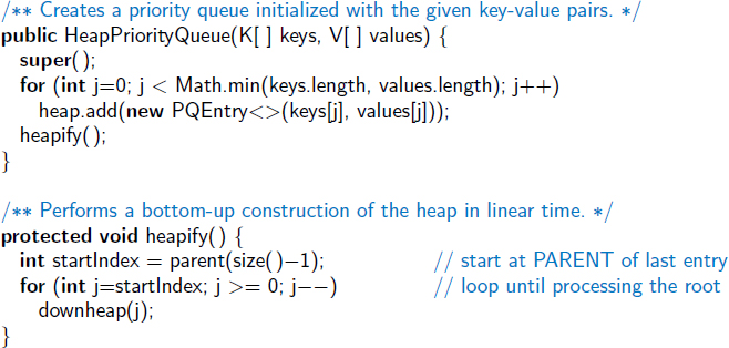
Code Fragment 9.10: Revision to the HeapPriorityQueue class of Code Fragments 9.8 and 9.9, supporting linear-time construction given an initial collection of key-value pairs.

Asymptotic Analysis of Bottom-Up Heap Construction

Bottom-up heap construction is asymptotically faster than incrementally inserting n entries into an initially empty heap. Intuitively, we are performing a single downheap operation at each position in the tree, rather than a single up-heap operation from each. Since more nodes are closer to the bottom of a tree than the top, the sum of the downward paths is linear, as shown in the following proposition.

Proposition 9.3: Bottom-up construction of a heap with n entries takes O(n) time, assuming two keys can be compared in O(1) time.

Justification: The primary cost of the construction is due to the down-heap steps performed at each nonleaf position. Let π_v denote the path of T from nonleaf node v to its “inorder successor” leaf, that is, the path that starts at v, goes to the right child of v, and then goes down leftward until it reaches a leaf. Although, π_v is not necessarily the path followed by the down-heap bubbling step from v, its number of edges is proportional to the height of the subtree rooted at v, and thus a bound on the complexity of the down-heap operation at v. The total running time of the bottom-up heap construction algorithm is therefore bounded by the sum . For intuition, Figure 9.6 illustrates the justification “visually,” marking each edge with the label of the nonleaf node v whose path π_v contains that edge.

We claim that the paths π_v for all nonleaf v are edge-disjoint, and thus the sum of the path lengths is bounded by the number of total edges in the tree, hence O(n). To show this, we consider what we term “right-leaning” and “left-leaning” edges (i.e., those going from a parent to a right, respectively left, child). A particular rightleaning edge e can only be part of the path π_v for node v that is the parent in the relationship represented by e. Left-leaning edges can be partitioned by considering the leaf that is reached if continuing down leftward until reaching a leaf. Each nonleaf node only uses left-leaning edges in the group leading to that nonleaf node's inorder successor. Since each nonleaf node must have a different inorder successor, no two such paths can contain the same left-leaning edge. We conclude that the bottom-up construction of heap T takes O(n) time.

Figure 9.6: Visual justification of the linear running time of bottom-up heap construction. Each edge e is labeled with a node v for which π_v contains e (if any).

9.3.5 Using the java.util.PriorityQueue Class

There is no priority queue interface built into Java, but Java does include a class, java.util.PriorityQueue, which implements the java.util.Queue interface. Instead of adding and removing elements according to the standard FIFO policy used by most queues, the java.util.PriorityQueue class processes its entries according to a priority The “front” of the queue will always be a minimal element, with priorities based either on the natural ordering of the elements, or in accordance with a comparator object sent as a parameter when constructing the priority queue.

The most notable difference between the java.util.PriorityQueue class and our own priority queue ADT is the model for managing keys and values. Whereas our public interface distinguishes between keys and values, the java.util.PriorityQueue class relies on a single element type. That element is effectively treated as a key.

If a user wishes to insert distinct keys and values, the burden is on the user to define and insert appropriate composite objects, and to ensure that those objects can be compared based on their keys. (The Java Collections Framework does include its own entry interface, java.util.Map.Entry, and a concrete implementation in the java.util.AbstractMap.SimpleEntry class; we discuss the map ADT in the next chapter.)

Table 9.4 shows the correspondance between methods of our priority queue ADT and those of the java.util.PriorityQueue class. The java.util.PriorityQueue class is implemented with a heap, so it guarantees O(log n)-time performance for methods add and remove, and constant-time performance for accessors peek, size, and isEmpty. In addition, it provides a parameterized method, remove(e), that removes a specific element e from the priority queue. However, that method runs in O(n) time, performing a sequential search to locate the element within the heap. (In Section 9.5, we extend our heap-based priority queue implementation to support a more efficient means for removing an arbitrary entry, or for updating the priority of an existing entry.)

Our Priority Queue ADT	java.util.PriorityQueue Class
insert(k,v)	add(new SimpleEntry(k,v))
min()	peek()
removeMin()	remove()
size()	size()
isEmpty()	isEmpty()

Table 9.4: Methods of our priority queue ADT and the corresponding methods when using the java.util.PriorityQueue class.

9.4 Sorting with a Priority Queue

One application of priority queues is sorting, where we are given a sequence of elements that can be compared according to a total order relation, and we want to rearrange them in increasing order (or at least in nondecreasing order if there are ties). The algorithm for sorting a sequence S with a priority queue P is quite simple and consists of the following two phases:

1. In the first phase, we insert the elements of S as keys into an initially empty priority queue P by means of a series of n insert operations, one for each element.
2. In the second phase, we extract the elements from P in nondecreasing order by means of a series of n removeMin operations, putting them back into S in that order.

A Java implementation of this algorithm is given in Code Fragment 9.11, assuming that the sequence is stored as a positional list. (Code for a different type of collection, such as an array or an array list, would be similar.)

The algorithm works correctly for any priority queue P, no matter how P is implemented. However, the running time of the algorithm is determined by the running times of operations insert and removeMin, which do depend on how P is implemented. Indeed, pqSort should be considered more a sorting “scheme” than a sorting “algorithm,” because it does not specify how the priority queue P is implemented. The pqSort scheme is the paradigm of several popular sorting algorithms, including selection-sort, insertion-sort, and heap-sort, which we will discuss in this section.

Code Fragment 9.11: An implementation of a pqSort method that sorts elements of a positional list using an initially empty priority queue to produce the ordering.

9.4.1 Selection-Sort and Insertion-Sort

We next demonstrate how the pqSort scheme results in two classic sorting algorithms when using an unsorted or sorted list for a priority queue.

Selection-Sort

In Phase 1 of the pqSort scheme, we insert all elements into a priority queue P; in Phase 2 we repeatedly remove the minimal element from P using the removeMin method. If we implement P with an unsorted list, then Phase 1 of pqSort takes O(n) time, for we can insert each element in O(1) time. In Phase 2, the running time of each removeMin operation is proportional to the size of P. Thus, the bottleneck computation is the repeated “selection” of the minimum element in Phase 2. For this reason, this algorithm is better known as selection-sort. (See Figure 9.7.)

Figure 9.7: Execution of selection-sort on sequence S = (7, 4, 8, 2, 5, 3, 9).

As noted above, the bottleneck is in Phase 2 where we repeatedly remove an entry with smallest key from the priority queue P. The size of P starts at n and incrementally decreases with each removeMin until it becomes 0. Thus, the first removeMin operation takes time O(n), the second one takes time O(n−1), and so on, until the last (n^th) operation takes time O(1). Therefore, the total time needed for the second phase is

By Proposition 4.3, we have . Thus, Phase 2 takes time O(n²), as does the entire selection-sort algorithm.

Insertion-Sort

If we implement the priority queue P using a sorted list, then the running time of Phase 2 improves to O(n), for each operation removeMin on P now takes O(1) time. Unfortunately, Phase 1 now becomes the bottleneck for the running time, since, in the worst case, each insert operation takes time proportional to the size of P. This sorting algorithm is therefore better known as insertion-sort (see Figure 9.8), for the bottleneck in this sorting algorithm involves the repeated “insertion” of a new element at the appropriate position in a sorted list.

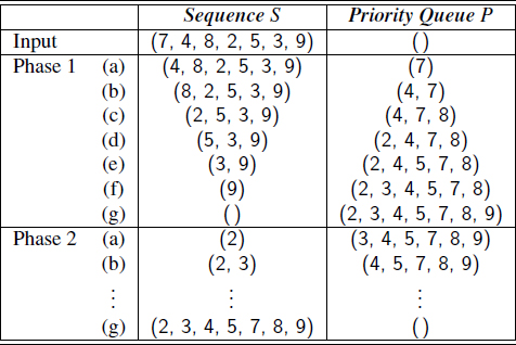
Figure 9.8: Execution of insertion-sort on sequence S = (7, 4, 8, 2, 5, 3, 9). In Phase 1, we repeatedly remove the first element of S and insert it into P. In Phase 2, we repeatedly perform the removeMin operation on P and add the returned element to the end of S.

Analyzing the running time of Phase 1 of insertion-sort, we note that it is

Again, by recalling Proposition 4.3, Phase 1 runs in O(n²) time, and hence, so does the entire insertion-sort algorithm.

Alternatively, we could change our definition of insertion-sort so that we insert elements starting from the end of the priority-queue list in Phase 1, in which case performing insertion-sort on a sequence that is already sorted would run in O(n) time. Indeed, the running time of insertion-sort in this case is O(n + I), where I is the number of inversions in the sequence, that is, the number of pairs of elements that start out in the input sequence in the wrong relative order.

9.4.2 Heap-Sort

As we have previously observed, realizing a priority queue with a heap has the advantage that all the methods in the priority queue ADT run in logarithmic time or better. Hence, this realization is suitable for applications where fast running times are sought for all the priority queue methods. Therefore, let us again consider the pqSort scheme, this time using a heap-based implementation of the priority queue.

During Phase 1, the i^th insert operation takes O(log i) time, since the heap has i entries after the operation is performed. Therefore, this phase takes O(nlog n) time. (It could be improved to O(n) with the bottom-up heap construction described in Section 9.3.4.)

During the second phase of method pqSort, the j^th removeMin operation runs in O(log(n−j + 1)), since the heap has n−j + 1 entries at the time the operation is performed. Summing over all j, this phase takes O(nlog n) time, so the entire priority-queue sorting algorithm runs in O(nlog n) time when we use a heap to implement the priority queue. This sorting algorithm is better known as heap-sort, and its performance is summarized in the following proposition.

Proposition 9.4: The heap-sort algorithm sorts a sequence S of n elements in O(n log n) time, assuming two elements of S can be compared in O(1) time.

Let us stress that the O(n log n) running time of heap-sort is considerably better than the O(n²) running time of selection-sort and insertion-sort.

Implementing Heap-Sort In-Place

If the sequence S to be sorted is implemented by means of an array-based sequence, such as an ArrayList in Java, we can speed up heap-sort and reduce its space requirement by a constant factor by using a portion of the array itself to store the heap, thus avoiding the use of an auxiliary heap data structure. This is accomplished by modifying the algorithm as follows:

1. We redefine the heap operations to be a maximum-oriented heap, with each position key being at least as large as its children. This can be done by recoding the algorithm, or by providing a new comparator that reverses the outcome of each comparison. At any time during the execution of the algorithm, we use the left portion of S, up to a certain index i−1, to store the entries of the heap, and the right portion of S, from index i to n−1, to store the elements of the sequence. Thus, the first i elements of S (at indices 0,...,i−1) provide the array-list representation of the heap.
2. In the first phase of the algorithm, we start with an empty heap and move the boundary between the heap and the sequence from left to right, one step at a time. In step i, for i = 1, ..., n, we expand the heap by adding the element at index i−1.
3. In the second phase of the algorithm, we start with an empty sequence and move the boundary between the heap and the sequence from right to left, one step at a time. At step i, for i = 1, ..., n, we remove a maximal element from the heap and store it at index n−i.

In general, we say that a sorting algorithm is in-place if it uses only a small amount of memory in addition to the sequence storing the objects to be sorted. The variation of heap-sort above qualifies as in-place; instead of transferring elements out of the sequence and then back in, we simply rearrange them. We illustrate the second phase of in-place heap-sort in Figure 9.9.

Figure 9.9: Phase 2 of an in-place heap-sort. The heap portion of each sequence representation is highlighted. The binary tree that each sequence (implicitly) represents is diagrammed with the most recent path of down-heap bubbling highlighted.

9.5 Adaptable Priority Queues

The methods of the priority queue ADT given in Section 9.1.2 are sufficient for most basic applications of priority queues, such as sorting. However, there are situations in which additional methods would be useful, as shown by the scenarios below involving the standby airline passenger application.

• A standby passenger with a pessimistic attitude may become tired of waiting and decide to leave ahead of the boarding time, requesting to be removed from the waiting list. Thus, we would like to remove from the priority queue the entry associated with this passenger. Operation removeMin does not suffice since the passenger leaving does not necessarily have first priority. Instead, we want a new operation, remove, that removes an arbitrary entry.
• Another standby passenger finds her gold frequent-flyer card and shows it to the agent. Thus, her priority has to be modified accordingly. To achieve this change of priority, we would like to have a new operation replaceKey allowing us to replace the key of an existing entry with a new key.
• Finally, a third standby passenger notices her name is misspelled on the ticket and asks it to be corrected. To perform this change, we need to update the passenger's record. Hence, we would like to have a new operation replace-Value, allowing us to replace the value of an existing entry with a new value.

The Adaptable Priority Queue ADT

The above scenarios motivate the definition of a new adaptable priority queue ADT that extends the priority queue ADT with additional functionality. We will see another application of adaptable priority queues when implementing certain graph algorithms in Sections 14.6.2 and 14.7.1.

In order to implement methods remove, replaceKey, and replaceValue efficiently, we need a mechanism for finding a user's element within a priority queue, ideally in a way that avoids performing a linear search through the entire collection. In the original definition of the priority queue ADT, a call to insert(k, v) formally returns an instance of type Entry to the user. In order to be able to update or remove an entry in our new adaptable priority queue ADT, the user must retain that Entry object as a token that can be sent back as a parameter to identify the relevant entry. Formally, the adaptable priority queue ADT includes the following methods (in addition to those of the standard priority queue):

remove(e):	Removes entry e from the priority queue.
replaceKey(e, k):	Replaces the key of existing entry e with k.
replaceValue(e, v):	Replaces the value of existing entry e with v.

An error occurs with each of these methods if parameter e is invalid (for example, because it had previously been removed from the priority queue).

9.5.1 Location-Aware Entries

To allow an entry instance to encode a location within a priority queue, we extend the PQEntry class (originally defined with the AbstractPriorityQueue base class), adding a third field that designates the current index of an entry within the array-based representation of the heap, as shown in Figure 9.10. (This approach is similar to our recommendation, on page 281, for implementing the positional list abstraction with an array.)

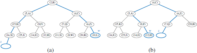
Figure 9.10: Representing a heap using an array of location-aware entries. The third field of each entry instance corresponds to the index of that entry within the array. Identifier token is presumed to be an entry reference in the user's scope.

When we perform priority queue operations on our heap, causing entries to be relocated within our structure, we must make sure to update the third field of each affected entry to reflect its new index within the array. As an example, Figure 9.11 shows the state of the above heap after a call to removeMin( ). The heap operation causes the minimal entry, (4,C), to be removed, and the last entry, (16,X), to be temporarily moved from the last position to the root, followed by a down-heap bubble phase. During the down-heap, element (16,X) is swapped with its left child, (5,A), at index 1 of the list, then swapped with its right child, (9,F), at index 4 of the list. In the final configuration, the last field for all affected entries has been modified to reflect their new location.

Figure 9.11: The result of a call to removeMin() on the heap originally portrayed in Figure 9.10. Identifier token continues to reference the same entry as in the original configuration, but the placement of that entry in the array has changed, as has the third field of the entry.

9.5.2 Implementing an Adaptable Priority Queue

Code Fragments 9.12 and 9.13 present a Java implementation of an adaptable priority queue, as a subclass of the HeapPriorityQueue class from Section 9.3.2. We begin by defining a nested AdaptablePQEntry class (lines 5–15) that extends the inherited PQEntry class, augmenting it with an additional index field. The inherited insert method is overridden, so that we create and initialize an instance of the AdaptablePQEntry class (not the original PQEntry class).

An important aspect of our design is that the original HeapPriorityQueue class relies exclusively on a protected swap method for all low-level data movement during up-heap or down-heap operations. The AdaptablePriorityQueue class overrides that utility in order to update the stored indices of our location-aware entries when they are relocated (as discussed on the previous page).

When an entry is sent as a parameter to remove, replaceKey, or replaceValue, we rely on the new index field of that entry to designate where the element resides in the heap (a fact that is easily validated). When a key of an existing entry is replaced, that new key may violate the heap-order property by being either too big or too small. We provide a new bubble utility that determines whether an upheap or down-heap bubbling step is warranted. When removing an arbitrary entry, we replace it with the last entry in the heap (to maintain the complete binary tree property) and perform the bubbling step, since the displaced element may have a key that is too large or too small for its new location.

Performance of Adaptable Priority Queue Implementations

The performance of an adaptable priority queue by means of our location-aware heap structure is summarized in Table 9.5. The new class provides the same asymptotic efficiency and space usage as the nonadaptive version, and provides logarithmic performance for the new locator-based remove and replaceKey methods, and constant-time performance for the new replaceValue method.

Method	Running Time
size, isEmpty, min	O(1)
insert	O(log n)
remove	O(log n)
removeMin	O(log n)
replaceKey	O(log n)
replaceValue	O(1)

Table 9.5: Running times of the methods of an adaptable priority queue with size n, realized by means of our array-based heap representation. The space requirement is O(n).

Code Fragment 9.12: An implementation of an adaptable priority queue. (Continues in Code Fragment 9.13.) This extends the HeapPriorityQueue class of Code Fragments 9.8 and 9.9.

Code Fragment 9.13: An implementation of an adaptable priority queue (continued from Code Fragment 9.12).

9.6 Exercises

Reinforcement

R-9.1	How long would it take to remove the smallest elements from a heap that contains n entries, using the removeMin operation?
R-9.2	Suppose you set the key for each position p of a binary tree T equal to its preorder rank. Under what circumstances is T a heap?
R-9.3	What does each removeMin call return within the following sequence of priority queue ADT operations: insert(5, A), insert(4, B), insert(7, F), insert(1, D), removeMin(), insert(3, J), insert(6, L), removeMin(), removeMin(), insert(8, G), removeMin(), insert(2, H), removeMin(), removeMin()?
R-9.4	An airport is developing a computer simulation of air-traffic control that handles events such as landings and takeoffs. Each event has a time stamp that denotes the time when the event will occur. The simulation program needs to efficiently perform the following two fundamental operations: Insert an event with a given time stamp (that is, add a future event). Extract the event with smallest time stamp (that is, determine the next event to process). Which data structure should be used for the above operations? Why?
R-9.5	The min method for the UnsortedPriorityQueue class executes in O(n) time, as analyzed in Table 9.2. Give a simple modification to the class so that min runs in O(1) time. Explain any necessary modifications to other methods of the class.
R-9.6	Can you adapt your solution to the previous problem to make removeMin run in O(1) time for the UnsortedPriorityQueue class? Explain your answer.
R-9.7	Illustrate the execution of the selection-sort algorithm on the following input sequence: (22, 15, 36, 44, 10, 3, 9, 13, 29, 25).
R-9.8	Illustrate the execution of the insertion-sort algorithm on the input sequence of the previous problem.
R-9.9	Give an example of a worst-case sequence with n elements for insertion-sort, and show that insertion-sort runs in Ω(n2) time on such a sequence.
R-9.10	At which positions of a heap might the third smallest key be stored?
R-9.11	At which positions of a heap might the largest key be stored?
R-9.12	Consider a situation in which a user has numeric keys and wishes to have a priority queue that is maximum-oriented. How could a standard (min-oriented) priority queue be used for such a purpose?
R-9.13	Illustrate the execution of the in-place heap-sort algorithm on the following input sequence: (2, 5, 16, 4, 10, 23, 39, 18, 26, 15).
R-9.14	Let T be a complete binary tree such that position p stores an element with key f(p), where f(p) is the level number of p (see Section 8.3.2). Is tree T a heap? Why or why not?
R-9.15	Explain why the description of down-heap bubbling does not consider the case in which position p has a right child but not a left child.
R-9.16	Is there a heap H storing seven entries with distinct keys such that a preorder traversal of H yields the entries of H in increasing or decreasing order by key? How about an inorder traversal? How about a postorder traversal? If so, give an example; if not, say why.
R-9.17	Let H be a heap storing 15 entries using the array-based representation of a complete binary tree. What is the sequence of indices of the array that are visited in a preorder traversal of H? What about an inorder traversal of H? What about a postorder traversal of H?
R-9.18	Show that the sum , appearing in the analysis of heap-sort, is Ω(n log n).
R-9.19	Bill claims that a preorder traversal of a heap will list its keys in nondecreasing order. Draw an example of a heap that proves him wrong.
R-9.20	Hillary claims that a postorder traversal of a heap will list its keys in nonincreasing order. Draw an example of a heap that proves her wrong.
R-9.21	Illustrate all the steps of the adaptable priority queue call remove(e) for entry e storing (16,X) in the heap of Figure 9.1.
R-9.22	Illustrate all the steps of the adaptable priority queue call replaceKey(e, 18) for entry e storing (5, A) in the heap of Figure 9.1.
R-9.23	Draw an example of a heap whose keys are all the odd numbers from 1 to 59 (with no repeats), such that the insertion of an entry with key 32 would cause up-heap bubbling to proceed all the way up to a child of the root (replacing that child's key with 32).
R-9.24	Describe a sequence of n insertions in a heap that requires Ω(nlog n) time to process.

Creativity

C-9.25	Show how to implement the stack ADT using only a priority queue and one additional integer instance variable.
C-9.26	Show how to implement the FIFO queue ADT using only a priority queue and one additional integer instance variable.
C-9.27	Professor Idle suggests the following solution to the previous problem. Whenever an entry is inserted into the queue, it is assigned a key that is equal to the current size of the queue. Does such a strategy result in FIFO semantics? Prove that it is so or provide a counterexample.
C-9.28	Reimplement the SortedPriorityQueue using a Java array. Make sure to maintain removeMin's O(1) performance.
C-9.29	Give an alternative implementation of the HeapPriorityQueue's upheap method that uses recursion (and no loop).
C-9.30	Give an implementation of the HeapPriorityQueue's downheap method that uses recursion (and no loop).
C-9.31	Assume that we are using a linked representation of a complete binary tree T, and an extra reference to the last node of that tree. Show how to update the reference to the last node after operations insert or remove in O(log n) time, where n is the current number of nodes of T. Be sure to handle all possible cases, as illustrated in Figure 9.12.
C-9.32	When using a linked-tree representation for a heap, an alternative method for finding the last node during an insertion in a heap T is to store, in the last node and each leaf node of T, a reference to the leaf node immediately to its right (wrapping to the first node in the next lower level for the rightmost leaf node). Show how to maintain such references in O(1) time per operation of the priority queue ADT assuming that T is implemented with a linked structure.
C-9.33	We can represent a path from the root to a given node of a binary tree by means of a binary string, where 0 means “go to the left child” and 1 means “go to the right child.” For example, the path from the root to the node storing (8,W) in the heap of Figure 9.12a is represented by “101.” Design an O(log n)-time algorithm for finding the last node of a complete binary tree with n nodes, based on the above representation. Show how this algorithm can be used in the implementation of a complete binary tree by means of a linked structure that does not keep an explicit reference to the last node instance.
C-9.34	Given a heap H and a key k, give an algorithm to compute all the entries in H having a key less than or equal to k. For example, given the heap of Figure 9.12a and query k = 7, the algorithm should report the entries with keys 2, 4, 5, 6, and 7 (but not necessarily in this order). Your algorithm should run in time proportional to the number of entries returned, and should not modify the heap. Figure 9.12: Two cases of updating the last node in a complete binary tree after operation insert or remove. Node w is the last node before operation insert or after operation remove. Node z is the last node after operation insert or before operation remove.
C-9.35	Provide a justification of the time bounds in Table 9.5.
C-9.36	Give an alternative analysis of bottom-up heap construction by showing the following summation is O(1), for any positive integer h:
C-9.37	Suppose two binary trees, T1 and T2, hold entries satisfying the heap-order property (but not necessarily the complete binary tree property). Describe a method for combining T1 and T2 into a binary tree T, whose nodes hold the union of the entries in T1 and T2 and also satisfy the heap-order property. Your algorithm should run in time O(h1 + h2) where h1 and h2 are the respective heights of T1 and T2.
C-9.38	Tamarindo Airlines wants to give a first-class upgrade coupon to their top log n frequent flyers, based on the number of miles accumulated, where n is the total number of the airlines' frequent flyers. The algorithm they currently use, which runs in O(nlog n) time, sorts the flyers by the number of miles flown and then scans the sorted list to pick the top log n flyers. Describe an algorithm that identifies the top log n flyers in O(n) time.
C-9.39	Explain how the k largest elements from an unordered collection of size n can be found in time O(n+k log n) using a maximum-oriented heap.
C-9.40	Explain how the k largest elements from an unordered collection of size n can be found in time O(nlogk) using O(k) auxiliary space.
C-9.41	Write a comparator for nonnegative integers that determines order based on the number of 1's in each integer's binary expansion, so that i < j if the number of 1's in the binary representation of i is less than the number of 1's in the binary representation of j.
C-9.42	Implement the binarySearch algorithm (see Section 5.1.3) using a Comparator for an array with elements of generic type E.
C-9.43	Given a class, MinPriorityQueue, that implements the minimum-oriented priority queue ADT, provide an implementation of a MaxPriorityQueue class that adapts to provide a maximum-oriented abstraction with methods insert, max, and removeMax. Your implementation should not make any assumption about the internal workings of the original MinPriorityQueue class, nor the type of keys that might be used.
C-9.44	Describe an in-place version of the selection-sort algorithm for an array that uses only O(1) space for instance variables in addition to the array.
C-9.45	Assuming the input to the sorting problem is given in an array A, describe how to implement the insertion-sort algorithm using only the array A and at most six additional (base-type) variables.
C-9.46	Give an alternate description of the in-place heap-sort algorithm using the standard minimum-oriented priority queue (instead of a maximum-oriented one).
C-9.47	A group of children want to play a game, called Unmonopoly, where in each turn the player with the most money must give half of his/her money to the player with the least amount of money. What data structure(s) should be used to play this game efficiently? Why?
C-9.48	An online computer system for trading stocks needs to process orders of the form “buy 100 shares at $x each” or “sell 100 shares at $y each.” A buy order for $x can only be processed if there is an existing sell order with price $y such that y ≤ x. Likewise, a sell order for $y can only be processed if there is an existing buy order with price $x such that y ≤ x. If a buy or sell order is entered but cannot be processed, it must wait for a future order that allows it to be processed. Describe a scheme that allows buy and sell orders to be entered in O(log n) time, independent of whether or not they can be immediately processed.
C-9.49	Extend a solution to the previous problem so that users are allowed to update the prices for their buy or sell orders that have yet to be processed.

Projects

P-9.50	Implement the in-place heap-sort algorithm. Experimentally compare its running time with that of the standard heap-sort that is not in-place.
P-9.51	Use the approach of either Exercise C-9.39 or C-9.40 to reimplement the method getFavorites of the FavoritesListMTF class from Section 7.7.2. Make sure that results are generated from largest to smallest.
P-9.52	Develop a Java implementation of an adaptable priority queue that is based on an unsorted list and supports location-aware entries.
P-9.53	Write an applet or stand-alone graphical program that animates a heap. Your program should support all the priority queue operations and should visualize the swaps in the up-heap and down-heap bubblings. (Extra: Visualize bottom-up heap construction as well.)
P-9.54	Write a program that can process a sequence of stock buy and sell orders as described in Exercise C-9.48.
P-9.55	One of the main applications of priority queues is in operating systems—for scheduling jobs on a CPU. In this project you are to build a program that schedules simulated CPU jobs. Your program should run in a loop, each iteration of which corresponds to a time slice for the CPU. Each job is assigned a priority, which is an integer between–20 (highest priority) and 19 (lowest priority), inclusive. From among all jobs waiting to be processed in a time slice, the CPU must work on a job with highest priority. In this simulation, each job will also come with a length value, which is an integer between 1 and 100, inclusive, indicating the number of time slices that are needed to process this job. For simplicity, you may assume jobs cannot be interrupted–once it is scheduled on the CPU, a job runs for a number of time slices equal to its length. Your simulator must output the name of the job running on the CPU in each time slice and must process a sequence of commands, one per time slice, each of which is of the form “add job name with length n and priority p” or “no new job this slice”.
P-9.56	Let S be a set of n points in the plane with distinct integer x- and y-coordinates. Let T be a complete binary tree storing the points from S at its external nodes, such that the points are ordered left to right by increasing x-coordinates. For each node v in T, let S(v) denote the subset of S consisting of points stored in the subtree rooted at v. For the root r of T, define top(r) to be the point in S = S(r) with maximal y-coordinate. For every other node v, define top(r) to be the point in S with highest y-coordinate in S(v) that is not also the highest y-coordinate in S(u), where u is the parent of v in T (if such a point exists). Such labeling turns T into a priority search tree. Describe a linear-time algorithm for turning T into a priority search tree. Implement this approach.

Chapter Notes

Knuth's book on sorting and searching [61] describes the motivation and history for the selection-sort, insertion-sort, and heap-sort algorithms. The heap-sort algorithm is due to Williams [95], and the linear-time heap construction algorithm is due to Floyd [35]. Additional algorithms and analyses for heaps and heap-sort variations can be found in papers by Bentley [14], Carlsson [21], Gonnet and Munro [39], McDiarmid and Reed [69], and Schaffer and Sedgewick [82].