
Chapter
10
Maps, Hash Tables, and Skip Lists
Contents
10.1.2 Application: Counting Word Frequencies
10.1.3 An AbstractMap Base Class
10.1.4 A Simple Unsorted Map Implementation
10.2.2 Collision-Handling Schemes
10.2.3 Load Factors, Rehashing, and Efficiency
10.2.4 Java Hash Table Implementation
10.3.2 Two Applications of Sorted Maps
10.4.1 Search and Update Operations in a Skip List
10.4.2 Probabilistic Analysis of Skip Lists ![]()
10.1 Maps
A map is an abstract data type designed to efficiently store and retrieve values based upon a uniquely identifying search key for each. Specifically, a map stores key-value pairs (k, v), which we call entries, where k is the key and v is its corresponding value. Keys are required to be unique, so that the association of keys to values defines a mapping. Figure 10.1 provides a conceptual illustration of a map using the file-cabinet metaphor. For a more modern metaphor, think about the web as being a map whose entries are the web pages. The key of a page is its URL (e.g., http://datastructures.net/) and its value is the page content.
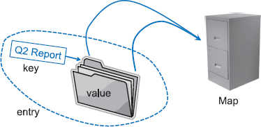
Figure 10.1: A conceptual illustration of the map ADT. Keys (labels) are assigned to values (folders) by a user. The resulting entries (labeled folders) are inserted into the map (file cabinet). The keys can be used later to retrieve or remove values.
Maps are also known as associative arrays, because the entry's key serves somewhat like an index into the map, in that it assists the map in efficiently locating the associated entry. However, unlike a standard array, a key of a map need not be numeric, and is does not directly designate a position within the structure. Common applications of maps include the following:
- A university's information system relies on some form of a student ID as a key that is mapped to that student's associated record (such as the student's name, address, and course grades) serving as the value.
- The domain-name system (DNS) maps a host name, such as www.wiley.com, to an Internet-Protocol (IP) address, such as 208.215.179.146.
- A social media site typically relies on a (nonnumeric) username as a key that can be efficiently mapped to a particular user's associated information.
- A company's customer base may be stored as a map, with a customer's account number or unique user ID as a key, and a record with the customer's information as a value. The map would allow a service representative to quickly access a customer's record, given the key.
- A computer graphics system may map a color name, such as 'turquoise', to the triple of numbers that describes the color's RGB (red-green-blue) representation, such as (64, 224, 208).
10.1.1 The Map ADT
Since a map stores a collection of objects, it should be viewed as a collection of key-value pairs. As an ADT, a map M supports the following methods:
| size(): | Returns the number of entries in M. |
| isEmpty(): | Returns a boolean indicating whether M is empty. |
| get(k): | Returns the value v associated with key k, if such an entry exists; otherwise returns null. |
| put(k, v): | If M does not have an entry with key equal to k, then adds entry (k, v) to M and returns null; else, replaces with v the existing value of the entry with key equal to k and returns the old value. |
| remove(k): | Removes from M the entry with key equal to k, and returns its value; if M has no such entry, then returns null. |
| keySet(): | Returns an iterable collection containing all the keys stored in M. |
| values(): | Returns an iterable collection containing all the values of entries stored in M (with repetition if multiple keys map to the same value). |
| entrySet(): | Returns an iterable collection containing all the key-value entries in M. |
Maps in the java.util Package
Our definition of the map ADT is a simplified version of the java.util.Map interface. For the elements of the iteration returned by entrySet, we will rely on the composite Entry interface introduced in Section 9.2.1 (the java.util.Map relies on the nested java.util.Map.Entry interface).
Notice that each of the operations get(k), put(k, v), and remove(k) returns the existing value associated with key k, if the map has such an entry, and otherwise returns null. This introduces ambiguity in an application for which null is allowed as a natural value associated with a key k. That is, if an entry (k, null) exists in a map, then the operation get(k) will return null, not because it couldn't find the key, but because it found the key and is returning its associated value.
Some implementations of the java.util.Map interface explicitly forbid use of a null value (and null keys, for that matter). However, to resolve the ambiguity when null is allowable, the interface contains a boolean method, containsKey(k) to definitively check whether k exists as a key. (We leave implementation of such a method as an exercise.)
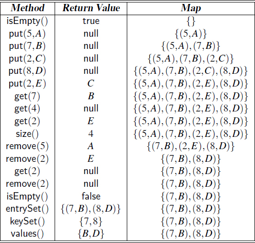
Example 10.1: In the following, we show the effect of a series of operations on an initially empty map storing entries with integer keys and single-character values.
A Java Interface for the Map ADT
A formal definition of a Java interface for our version of the map ADT is given in Code Fragment 10.1. It uses the generics framework (Section 2.5.2), with K designating the key type and V designating the value type.

Code Fragment 10.1: Java interface for our simplified version of the map ADT.
10.1.2 Application: Counting Word Frequencies
As a case study for using a map, consider the problem of counting the number of occurrences of words in a document. This is a standard task when performing a statistical analysis of a document, for example, when categorizing an email or news article. A map is an ideal data structure to use here, for we can use words as keys and word counts as values. We show such an application in Code Fragment 10.2.
We begin with an empty map, mapping words to their integer frequencies. (We rely on the ChainHashMap class that will be introduced in Section 10.2.4.) We first scan through the input, considering adjacent alphabetic characters to be words, which we then convert to lowercase. For each word found, we attempt to retrieve its current frequency from the map using the get method, with a yet unseen word having frequency zero. We then (re)set its frequency to be one more to reflect the current occurrence of the word. After processing the entire input, we loop through the entrySet() of the map to determine which word has the most occurrences.
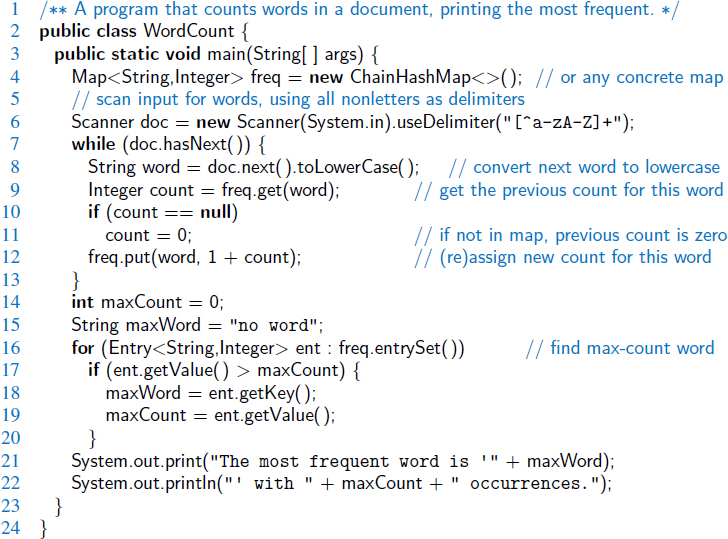
Code Fragment 10.2: A program for counting word frequencies in a document, printing the most frequent word. The document is parsed using the Scanner class, for which we change the delimiter for separating tokens from whitespace to any nonletter. We also convert words to lowercase.
10.1.3 An AbstractMap Base Class
In the remainder of this chapter (and the next), we will be providing many different implementations of the map ADT using a variety of data structures, each with its own trade-off of advantages and disadvantages. As we have done in earlier chapters, we rely on a combination of abstract and concrete classes in the interest of greater code reuse. Figure 10.2 provides a preview of those classes.

Figure 10.2: Our hierarchy of map types (with references to where they are defined).
We begin, in this section, by designing an AbstractMap base class that provides functionality that is shared by all of our map implementations. More specifically, the base class (given in Code Fragment 10.3) provides the following support:
- An implementation of the isEmpty method, based upon the presumed implementation of the size method.
- A nested MapEntry class that implements the public Entry interface, while providing a composite for storing key-value entries in a map data structure.
- Concrete implementations of the keySet and values methods, based upon an adaption to the entrySet method. In this way, concrete map classes need only implement the entrySet method to provide all three forms of iteration.
We implement the iterations using the technique introduced in Section 7.4.2 (at that time providing an iteration of all elements of a positional list given an iteration of all positions of the list).

Code Fragment 10.3: Implementation of the AbstractMap base class.
10.1.4 A Simple Unsorted Map Implementation
We demonstrate the use of the AbstractMap class with a very simple concrete implementation of the map ADT that relies on storing key-value pairs in arbitrary order within a Java ArrayList. The presentation of such an UnsortedTableMap class is given in Code Fragments 10.4 and 10.5.
Each of the fundamental methods get(k), put(k, v), and remove(k) requires an initial scan of the array to determine whether an entry with key equal to k exists. For this reason, we provide a nonpublic utility, findIndex(key), that returns the index at which such an entry is found, or −1 if no such entry is found. (See Code Fragment 10.4.)
The rest of the implementation is rather simple. One subtlety worth mentioning is the way in which we remove an entry from the array list. Although we could use the remove method of the ArrayList class, that would result in an unnecessary loop to shift all subsequent entries to the left. Because the map is unordered, we prefer to fill the vacated cell of the array by relocating the last entry to that location. Such an update step runs in constant time.
Unfortunately, the UnsortedTableMap class on the whole is not very efficient. On a map with n entries, each of the fundamental methods takes O(n) time in the worst case because of the need to scan through the entire list when searching for an existing entry. Fortunately, as we discuss in the next section, there is a much faster strategy for implementing the map ADT.

Code Fragment 10.4: An implementation of a map using a Java ArrayList as an unsorted table. (Continues in Code Fragment 10.5.) The parent class AbstractMap is given in Code Fragment 10.3.

Code Fragment 10.5: An implementation of a map using a Java ArrayList as an unsorted table (continued from Code Fragment 10.4).
10.2 Hash Tables
In this section, we introduce one of the most efficient data structures for implementing a map, and the one that is used most in practice. This structure is known as a hash table.
Intuitively, a map M supports the abstraction of using keys as “addresses” that help locate an entry. As a mental warm-up, consider a restricted setting in which a map with n entries uses keys that are known to be integers in a range from 0 to N − 1 for some N ≥ n. In this case, we can represent the map using a lookup table of length N, as diagrammed in Figure 10.3.

Figure 10.3: A lookup table with length 11 for a map containing entries (1,D), (3,Z), (6,C), and (7,Q).
In this representation, we store the value associated with key k at index k of the table (presuming that we have a distinct way to represent an empty slot). Basic map operations get, put, and remove can be implemented in O(1) worst-case time.
There are two challenges in extending this framework to the more general setting of a map. First, we may not wish to devote an array of length N if it is the case that ![]() . Second, we do not in general require that a map's keys be integers. The novel concept for a hash table is the use of a hash function to map general keys to corresponding indices in a table. Ideally, keys will be well distributed in the range from 0 to N − 1 by a hash function, but in practice there may be two or more distinct keys that get mapped to the same index. As a result, we will conceptualize our table as a bucket array, as shown in Figure 10.4, in which each bucket may manage a collection of entries that are sent to a specific index by the hash function. (To save space, an empty bucket may be replaced by a null reference.)
. Second, we do not in general require that a map's keys be integers. The novel concept for a hash table is the use of a hash function to map general keys to corresponding indices in a table. Ideally, keys will be well distributed in the range from 0 to N − 1 by a hash function, but in practice there may be two or more distinct keys that get mapped to the same index. As a result, we will conceptualize our table as a bucket array, as shown in Figure 10.4, in which each bucket may manage a collection of entries that are sent to a specific index by the hash function. (To save space, an empty bucket may be replaced by a null reference.)
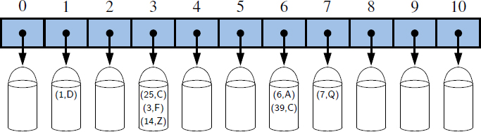
Figure 10.4: A bucket array of capacity 11 with entries (1,D), (25,C), (3,F), (14,Z), (6,A), (39,C), and (7,Q), using a simple hash function.
10.2.1 Hash Functions
The goal of a hash function, h, is to map each key k to an integer in the range [0,N − 1], where N is the capacity of the bucket array for a hash table. Equipped with such a hash function, h, the main idea of this approach is to use the hash function value, h(k), as an index into our bucket array, A, instead of the key k (which may not be appropriate for direct use as an index). That is, we store the entry (k, v) in the bucket A[h(k)].
If there are two or more keys with the same hash value, then two different entries will be mapped to the same bucket in A. In this case, we say that a collision has occurred. To be sure, there are ways of dealing with collisions, which we will discuss later, but the best strategy is to try to avoid them in the first place. We say that a hash function is “good” if it maps the keys in our map so as to sufficiently minimize collisions. For practical reasons, we also would like a hash function to be fast and easy to compute.
It is common to view the evaluation of a hash function, h(k), as consisting of two portions—a hash code that maps a key k to an integer, and a compression function that maps the hash code to an integer within a range of indices, [0, N − 1], for a bucket array. (See Figure 10.5.)

Figure 10.5: Two parts of a hash function: a hash code and a compression function.
The advantage of separating the hash function into two such components is that the hash code portion of that computation is independent of a specific hash table size. This allows the development of a general hash code for each object that can be used for a hash table of any size; only the compression function depends upon the table size. This is particularly convenient, because the underlying bucket array for a hash table may be dynamically resized, depending on the number of entries currently stored in the map. (See Section 10.2.3.)
Hash Codes
The first action that a hash function performs is to take an arbitrary key k in our map and compute an integer that is called the hash code for k; this integer need not be in the range [0,N − 1], and may even be negative. We desire that the set of hash codes assigned to our keys should avoid collisions as much as possible. For if the hash codes of our keys cause collisions, then there is no hope for our compression function to avoid them. In this subsection, we begin by discussing the theory of hash codes. Following that, we discuss practical implementations of hash codes in Java.
Treating the Bit Representation as an Integer
To begin, we note that, for any data type X that is represented using at most as many bits as our integer hash codes, we can simply take as a hash code for X an integer interpretation of its bits. Java relies on 32-bit hash codes, so for base types byte, short, int, and char, we can achieve a good hash code simply by casting a value to int. Likewise, for a variable x of base type float, we can convert x to an integer using a call to Float.floatToIntBits(x), and then use this integer as x's hash code.
For a type whose bit representation is longer than a desired hash code (such as Java's long and double types), the above scheme is not immediately applicable. One possibility is to use only the high-order 32 bits (or the low-order 32 bits). This hash code, of course, ignores half of the information present in the original key, and if many of the keys in our map only differ in these bits, then they will collide using this simple hash code.
A better approach is to combine in some way the high-order and low-order portions of a 64-bit key to form a 32-bit hash code, which takes all the original bits into consideration. A simple implementation is to add the two components as 32-bit numbers (ignoring overflow), or to take the exclusive-or of the two components. These approaches of combining components can be extended to any object x whose binary representation can be viewed as an n-tuple (x0, x1,..., xn−1) of 32-bit integers, for example, by forming a hash code for x as ![]() , or as x0 ⊕ x1 ⊕ ··· ⊕ xn−1, where the ⊕ symbol represents the bitwise exclusive-or operation (which is the ^ operator in Java).
, or as x0 ⊕ x1 ⊕ ··· ⊕ xn−1, where the ⊕ symbol represents the bitwise exclusive-or operation (which is the ^ operator in Java).
Polynomial Hash Codes
The summation and exclusive-or hash codes, described above, are not good choices for character strings or other variable-length objects that can be viewed as tuples of the form (x0, x1,..., xn−1), where the order of the xi's is significant. For example, consider a 16-bit hash code for a character string s that sums the Unicode values of the characters in s. This hash code unfortunately produces lots of unwanted collisions for common groups of strings. In particular, "temp01" and "temp10" collide using this function, as do "stop", "tops", "pots", and "spot". A better hash code should somehow take into consideration the positions of the xi's. An alternative hash code, which does exactly this, is to choose a nonzero constant, a ≠ 1, and use as a hash code the value
x0an−1 + x1an−2 + ··· + xn−2a + xn−1.
Mathematically speaking, this is simply a polynomial in a that takes the components (x0,x1,...,xn−1) of an object x as its coefficients. This hash code is therefore called a polynomial hash code. By Horner's rule (see Exercise C-4.54), this polynomial can be computed as
xn−1 + a(xn−2 + a(xn−3 + ··· + a(x2 + a(x1 + ax0)) ···)).
Intuitively, a polynomial hash code uses multiplication by different powers as a way to spread out the influence of each component across the resulting hash code.
Of course, on a typical computer, evaluating a polynomial will be done using the finite bit representation for a hash code; hence, the value will periodically overflow the bits used for an integer. Since we are more interested in a good spread of the object x with respect to other keys, we simply ignore such overflows. Still, we should be mindful that such overflows are occurring and choose the constant a so that it has some nonzero, low-order bits, which will serve to preserve some of the information content even as we are in an overflow situation.
We have done some experimental studies that suggest that 33, 37, 39, and 41 are particularly good choices for a when working with character strings that are English words. In fact, in a list of over 50,000 English words formed as the union of the word lists provided in two variants of Unix, we found that taking a to be 33, 37, 39, or 41 produced fewer than 7 collisions in each case!
Cyclic-Shift Hash Codes
A variant of the polynomial hash code replaces multiplication by a with a cyclic shift of a partial sum by a certain number of bits. For example, a 5-bit cyclic shift of the 32-bit value 00111101100101101010100010101000 is achieved by taking the leftmost five bits and placing those on the rightmost side of the representation, resulting in 10110010110101010001010100000111. While this operation has little natural meaning in terms of arithmetic, it accomplishes the goal of varying the bits of the calculation. In Java, a cyclic shift of bits can be accomplished through careful use of the bitwise shift operators.
An implementation of a cyclic-shift hash code computation for a character string in Java appears as follows:
static int hashCode(String s) {
  int h=0;
  for (int i=0; i<s.length(); i++) {
    h = (h << 5) | (h >>> 27);             // 5-bit cyclic shift of the running sum
    h += (int) s.charAt(i);                // add in next character
  }
  return h;
}
As with the traditional polynomial hash code, fine-tuning is required when using a cyclic-shift hash code, as we must wisely choose the amount to shift by for each new character. Our choice of a 5-bit shift is justified by experiments run on a list of just over 230,000 English words, comparing the number of collisions for various shift amounts (see Table 10.1).

Table 10.1: Comparison of collision behavior for the cyclic-shift hash code as applied to a list of 230,000 English words. The “Total” column records the total number of words that collide with at least one other, and the “Max” column records the maximum number of words colliding at any one hash code. Note that with a cyclic shift of 0, this hash code reverts to the one that simply sums all the characters.
Hash Codes in Java
The notion of hash codes are an integral part of the Java language. The Object class, which serves as an ancestor of all object types, includes a default hashCode() method that returns a 32-bit integer of type int, which serves as an object's hash code. The default version of hashCode() provided by the Object class is often just an integer representation derived from the object's memory address.
However, we must be careful if relying on the default version of hashCode() when authoring a class. For hashing schemes to be reliable, it is imperative that any two objects that are viewed as “equal” to each other have the same hash code. This is important because if an entry is inserted into a map, and a later search is performed on a key that is considered equivalent to that entry's key, the map must recognize this as a match. (See, for example, the UnsortedTableMap.findlndex method in Code Fragment 10.4.) Therefore, when using a hash table to implement a map, we want equivalent keys to have the same hash code so that they are guaranteed to map to the same bucket. More formally, if a class defines equivalence through the equals method (see Section 3.5), then that class should also provide a consistent implementation of the hashCode method, such that if x.equals(y) then x.hashCode() == y.hashCode().
As an example, Java's String class defines the equals method so that two instances are equivalent if they have precisely the same sequence of characters. That class also overrides the hashCode method to provide consistent behavior. In fact, the implementation of hash codes for the String class is excellent. If we repeat the experiment from the previous page using Java's implementation of hash codes, there are only 12 collisions among more than 230,000 words. Java's primitive wrapper classes also define hashCode, using techniques described on page 412.
As an example of how to properly implement hashCode for a user-defined class, we will revisit the SinglyLinkedList class from Chapter 3. We defined the equals method for that class, in Section 3.5.2, so that two lists are equivalent if they represent equal-length sequences of elements that are pairwise equivalent. We can compute a robust hash code for a list by taking the exclusive-or of its elements' hash codes, while performing a cyclic shift. (See Code Fragment 10.6.)

Code Fragment 10.6: A robust implementation of the hashCode method for the SinglyLinkedList class from Chapter 3.
Compression Functions
The hash code for a key k will typically not be suitable for immediate use with a bucket array, because the integer hash code may be negative or may exceed the capacity of the bucket array. Thus, once we have determined an integer hash code for a key object k, there is still the issue of mapping that integer into the range [0, N − 1]. This computation, known as a compression function, is the second action performed as part of an overall hash function. A good compression function is one that minimizes the number of collisions for a given set of distinct hash codes.
The Division Method
A simple compression function is the division method, which maps an integer i to
i mod N,
where N, the size of the bucket array, is a fixed positive integer. Additionally, if we take N to be a prime number, then this compression function helps “spread out” the distribution of hashed values. Indeed, if N is not prime, then there is greater risk that patterns in the distribution of hash codes will be repeated in the distribution of hash values, thereby causing collisions. For example, if we insert keys with hash codes {200, 205, 210, 215, 220,..., 600} into a bucket array of size 100, then each hash code will collide with three others. But if we use a bucket array of size 101, then there will be no collisions. If a hash function is chosen well, it should ensure that the probability of two different keys getting hashed to the same bucket is 1/N. Choosing N to be a prime number is not always enough, however, for if there is a repeated pattern of hash codes of the form pN + q for several different p's, then there will still be collisions.
The MAD Method
A more sophisticated compression function, which helps eliminate repeated patterns in a set of integer keys, is the Multiply-Add-and-Divide (or “MAD”)method. This method maps an integer i to
[(ai + b) mod p] mod N,
where N is the size of the bucket array, p is a prime number larger than N, and a and b are integers chosen at random from the interval [0, p − 1], with a > 0. This compression function is chosen in order to eliminate repeated patterns in the set of hash codes and get us closer to having a “good” hash function, that is, one such that the probability any two different keys collide is 1/N. This good behavior would be the same as we would have if these keys were “thrown” into A uniformly at random.
10.2.2 Collision-Handling Schemes
The main idea of a hash table is to take a bucket array, A, and a hash function, h, and use them to implement a map by storing each entry (k, v) in the “bucket” A[h(k)]. This simple idea is challenged, however, when we have two distinct keys, k1 and k2, such that h(k1) = h(k2). The existence of such collisions prevents us from simply inserting a new entry (k, v) directly into the bucket A[h(k)]. It also complicates our procedure for performing insertion, search, and deletion operations.
Separate Chaining
A simple and efficient way for dealing with collisions is to have each bucket A[j] store its own secondary container, holding all entries (k, v) such that h(k) = j. A natural choice for the secondary container is a small map instance implemented using an unordered list, as described in Section 10.1.4. This collision resolution rule is known as separate chaining, and is illustrated in Figure 10.6.

Figure 10.6: A hash table of size 13, storing 10 entries with integer keys, with collisions resolved by separate chaining. The compression function is h(k) = k mod 13. For simplicity, we do not show the values associated with the keys.
In the worst case, operations on an individual bucket take time proportional to the size of the bucket. Assuming we use a good hash function to index the n entries of our map in a bucket array of capacity N, the expected size of a bucket is n/N. Therefore, if given a good hash function, the core map operations run in ![]() . The ratio λ = n/N, called the load factor of the hash table, should be bounded by a small constant, preferably below 1. As long as λ is O(1), the core operations on the hash table run in O(1) expected time.
. The ratio λ = n/N, called the load factor of the hash table, should be bounded by a small constant, preferably below 1. As long as λ is O(1), the core operations on the hash table run in O(1) expected time.
Open Addressing
The separate chaining rule has many nice properties, such as affording simple implementations of map operations, but it nevertheless has one slight disadvantage: It requires the use of an auxiliary data structure to hold entries with colliding keys. If space is at a premium (for example, if we are writing a program for a small handheld device), then we can use the alternative approach of storing each entry directly in a table slot. This approach saves space because no auxiliary structures are employed, but it requires a bit more complexity to properly handle collisions. There are several variants of this approach, collectively referred to as open addressing schemes, which we discuss next. Open addressing requires that the load factor is always at most 1 and that entries are stored directly in the cells of the bucket array itself.
Linear Probing and Its Variants
A simple method for collision handling with open addressing is linear probing. With this approach, if we try to insert an entry (k, v) into a bucket A [j] that is already occupied, where j = h(k), then we next try A[(j + 1) mod N]. If A[(j + 1) mod N] is also occupied, then we try A[(j + 2) mod N], and so on, until we find an empty bucket that can accept the new entry. Once this bucket is located, we simply insert the entry there. Of course, this collision resolution strategy requires that we change the implementation when searching for an existing key—the first step of all get, put, or remove operations. In particular, to attempt to locate an entry with key equal to k, we must examine consecutive slots, starting from A[h(k)], until we either find an entry with an equal key or we find an empty bucket. (See Figure 10.7.) The name “linear probing” comes from the fact that accessing a cell of the bucket array can be viewed as a “probe,” and that consecutive probes occur in neighboring cells (when viewed circularly).

Figure 10.7: Insertion into a hash table with integer keys using linear probing. The hash function is h(k) = k mod 11. Values associated with keys are not shown.
To implement a deletion, we cannot simply remove a found entry from its slot in the array. For example, after the insertion of key 15 portrayed in Figure 10.7, if the entry with key 37 were trivially deleted, a subsequent search for 15 would fail because that search would start by probing at index 4, then index 5, and then index 6, at which an empty cell is found. A typical way to get around this difficulty is to replace a deleted entry with a special “defunct” sentinel object. With this special marker possibly occupying spaces in our hash table, we modify our search algorithm so that the search for a key k will skip over cells containing the defunct sentinel and continue probing until reaching the desired entry or an empty bucket (or returning back to where we started from). Additionally, our algorithm for put should remember a defunct location encountered during the search for k, since this is a valid place to put a new entry (k, v), if no existing entry is found beyond it.
Although use of an open addressing scheme can save space, linear probing suffers from an additional disadvantage. It tends to cluster the entries of a map into contiguous runs, which may even overlap (particularly if more than half of the cells in the hash table are occupied). Such contiguous runs of occupied hash cells cause searches to slow down considerably.
Another open addressing strategy, known as quadratic probing, iteratively tries the buckets A[(h(k) + f(i)) mod N], for i = 0,1,2,..., where f(i) = i2, until finding an empty bucket. As with linear probing, the quadratic probing strategy complicates the removal operation, but it does avoid the kinds of clustering patterns that occur with linear probing. Nevertheless, it creates its own kind of clustering, called secondary clustering, where the set of filled array cells still has a nonuniform pattern, even if we assume that the original hash codes are distributed uniformly. When N is prime and the bucket array is less than half full, the quadratic probing strategy is guaranteed to find an empty slot. However, this guarantee is not valid once the table becomes at least half full, or if N is not chosen as a prime number; we explore the cause of this type of clustering in an exercise (C-10.42).
An open addressing strategy that does not cause clustering of the kind produced by linear probing or the kind produced by quadratic probing is the double hashing strategy. In this approach, we choose a secondary hash function, h′, and if h maps some key k to a bucket A[h(k)] that is already occupied, then we iteratively try the buckets A[(h(k) + f(i)) mod N] next, for i = 1,2,3,..., where f(i) = i · h′(k). In this scheme, the secondary hash function is not allowed to evaluate to zero; a common choice is h′(k) = q − (k mod q), for some prime number q < N. Also, N should be a prime.
Another approach to avoid clustering with open addressing is to iteratively try buckets A[(h(k) + f(i)) mod N] where f(i) is based on a pseudorandom number generator, providing a repeatable, but somewhat arbitrary, sequence of subsequent probes that depends upon bits of the original hash code.
10.2.3 Load Factors, Rehashing, and Efficiency
In the hash table schemes described thus far, it is important that the load factor, λ = n/N, be kept below 1. With separate chaining, as λ gets very close to 1, the probability of a collision greatly increases, which adds overhead to our operations, since we must revert to linear-time list-based methods in buckets that have collisions. Experiments and average-case analyses suggest that we should maintain λ < 0.9 for hash tables with separate chaining. (By default, Java's implementation uses separate chaining with λ < 0.75.)
With open addressing, on the other hand, as the load factor λ grows beyond 0.5 and starts approaching 1, clusters of entries in the bucket array start to grow as well. These clusters cause the probing strategies to “bounce around” the bucket array for a considerable amount of time before they find an empty slot. In Exercise C-10.42, we explore the degradation of quadratic probing when λ ≥ 0.5. Experiments suggest that we should maintain λ < 0.5 for an open addressing scheme with linear probing, and perhaps only a bit higher for other open addressing schemes.
If an insertion causes the load factor of a hash table to go above the specified threshold, then it is common to resize the table (to regain the specified load factor) and to reinsert all objects into this new table. Although we need not define a new hash code for each object, we do need to reapply a new compression function that takes into consideration the size of the new table. Rehashing will generally scatter the entries throughout the new bucket array. When rehashing to a new table, it is a good requirement for the new array's size to be a prime number approximately double the previous size (see Exercise C-10.32). In that way, the cost of rehashing all the entires in the table can be amortized against the time used to insert them in the first place (as with dynamic arrays; see Section 7.2.1).
Efficiency of Hash Tables
Although the details of the average-case analysis of hashing are beyond the scope of this book, its probabilistic basis is quite intuitive. If our hash function is good, then we expect the entries to be uniformly distributed in the N cells of the bucket array. Thus, to store n entries, the expected number of keys in a bucket would be ![]() , which is O(1) if n is O(N).
, which is O(1) if n is O(N).
The costs associated with a periodic rehashing (when resizing a table after occasional insertions or deletions) can be accounted for separately, leading to an additional O(1) amortized cost for put and remove.
In the worst case, a poor hash function could map every entry to the same bucket. This would result in linear-time performance for the core map operations with separate chaining, or with any open addressing model in which the secondary sequence of probes depends only on the hash code. A summary of these costs is given in Table 10.2.

Table 10.2: Comparison of the running times of the methods of a map realized by means of an unsorted list (as in Section 10.1.4) or a hash table. We let n denote the number of entries in the map, and we assume that the bucket array supporting the hash table is maintained such that its capacity is proportional to the number of entries in the map.
An Anecdote About Hashing and Computer Security
In a 2003 academic paper, researchers discuss the possibility of exploiting a hash table's worst-case performance to cause a denial-of-service (DoS) attack of Internet technologies. Since many published algorithms compute hash codes with a deterministic function, an attacker could precompute a very large number of moderate-length strings that all hash to the identical 32-bit hash code. (Recall that by any of the hashing schemes we describe, other than double hashing, if two keys are mapped to the same hash code, they will be inseparable in the collision resolution.) This concern was brought to the attention of the Java development team, and that of many other programming languages, but deemed an insignificant risk at the time by most. (Kudos to the Perl team for implementing a fix in 2003.)
In late 2011, another team of researchers demonstrated an implementation of just such an attack. Web servers allow a series of key-value parameters to be embedded in a URL using a syntax such as ?key1=val1&key2=val2&key3=val3. Those key-value pairs are strings and a typical Web server immediately stores them in a hash-map. Servers already place a limit on the length and number of such parameters, to avoid overload, but they presume that the total insertion time in the map will be linear in the number of entries, given the expected constant-time operations. However, if all keys were to collide, the insertions into the map will require quadratic time, causing the server to perform an inordinate amount of work.
In 2012, the OpenJDK team announced the following resolution: they distributed a security patch that includes an alternative hash function that introduces randomization into the computation of hash codes, making it less tractable to reverse engineer a set of colliding strings. However, to avoid breaking existing code, the new feature is disabled by default in Java SE 7 and, when enabled, is only used for hashing strings and only when a table size grows beyond a certain threshold. Enhanced hashing will be enabled in Java SE 8 for all types and uses.
10.2.4 Java Hash Table Implementation
In this section, we develop two implementations of a hash table, one using separate chaining and the other using open addressing with linear probing. While these approaches to collision resolution are quite different, there are many higher-level commonalities to the two hashing algorithms. For that reason, we extend the AbstractMap class (from Code Fragment 10.3) to define a new AbstractHashMap class (see Code Fragment 10.7), which provides much of the functionality common to our two hash table implementations.
We will begin by discussing what this abstract class does not do—it does not provide any concrete representation of a table of “buckets.” With separate chaining, each bucket will be a secondary map. With open addressing, however, there is no tangible container for each bucket; the “buckets” are effectively interleaved due to the probing sequences. In our design, the AbstractHashMap class presumes the following to be abstract methods—to be implemented by each concrete subclass:
| createTable(): | This method should create an initially empty table having size equal to a designated capacity instance variable. |
| bucketGet(h, k): | This method should mimic the semantics of the public get method, but for a key k that is known to hash to bucket h. |
| bucketPut(h, k, v): | This method should mimic the semantics of the public put method, but for a key k that is known to hash to bucket h. |
| bucketRemove(h, k): | This method should mimic the semantics of the public remove method, but for a key k known to hash to bucket h. |
| entrySet(): | This standard map method iterates through all entries of the map. We do not delegate this on a per-bucket basis because “buckets” in open addressing are not inherently disjoint. |
What the AbstractHashMap class does provide is mathematical support in the form of a hash compression function using a randomized Multiply-Add-and-Divide (MAD) formula, and support for automatically resizing the underlying hash table when the load factor reaches a certain threshold.
The hashValue method relies on an original key's hash code, as returned by its hashCode() method, followed by MAD compression based on a prime number and the scale and shift parameters that are randomly chosen in the constructor.
To manage the load factor, the AbstractHashMap class declares a protected member, n, which should equal the current number of entries in the map; however, it must rely on the subclasses to update this field from within methods bucketPut and bucketRemove. If the load factor of the table increases beyond 0.5, we request a bigger table (using the createTable method) and reinsert all entries into the new table. (For simplicity, this implementation uses tables of size 2k + 1, even though these are not generally prime.)

Code Fragment 10.7: A base class for our hash table implementations, extending the AbstractMap class from Code Fragment 10.3.
Separate Chaining
To represent each bucket for separate chaining, we use an instance of the simpler UnsortedTableMap class from Section 10.1.4. This technique, in which we use a simple solution to a problem to create a new, more advanced solution, is known as bootstrapping. The advantage of using a map for each bucket is that it becomes easy to delegate responsibilities for top-level map operations to the appropriate bucket.
The entire hash table is then represented as a fixed-capacity array A of the secondary maps. Each cell, A[h], is initially a null reference; we only create a secondary map when an entry is first hashed to a particular bucket.
As a general rule, we implement bucketGet(h, k) by calling A[h].get(k), we implement bucketPut(h, k, v) by calling A[h].put(k, v), and bucketRemove(h, k) by calling A[h].remove(k). However, care is needed for two reasons.
First, because we choose to leave table cells as null until a secondary map is needed, each of these fundamental operations must begin by checking to see if A[h] is null. In the case of bucketGet and bucketRemove, if the bucket does not yet exist, we can simply return null as there can not be any entry matching key k. In the case of bucketPut, a new entry must be inserted, so we instantiate a new UnsortedTableMap for A[h] before continuing.
The second issue is that, in our AbstractHashMap framework, the subclass has the responsibility to properly maintain the instance variable n when an entry is newly inserted or deleted. Remember that when put(k, v) is called on a map, the size of the map only increases if key k is new to the map (otherwise, the value of an existing entry is reassigned). Similarly, a call to remove(k) only decreases the size of the map when an entry with key equal to k is found. In our implementation, we determine the change in the overall size of the map, by determining if there is any change in the size of the relevant secondary map before and after an operation.
Code Fragment 10.8 provides a complete definition for our ChainHashMap class, which implements a hash table with separate chaining. If we assume that the hash function performs well, a map with n entries and a table of capacity N will have an expected bucket size of n/N (recall, this is its load factor). So even though the individual buckets, implemented as UnsortedTableMap instances, are not particularly efficient, each bucket has expected O(1) size, provided that n is O(N), as in our implementation. Therefore, the expected running time of operations get, put, and remove for this map is O(1). The entrySet method (and thus the related keySet and values) runs in O(n + N) time, as it loops through the length of the table (with length N) and through all buckets (which have cumulative lengths n).

Code Fragment 10.8: A concrete hash map implementation using separate chaining.
Linear Probing
Our implementation of a ProbeHashMap class, using open addressing with linear probing, is given in Code Fragments 10.9 and 10.10. In order to support deletions, we use a technique described in Section 10.2.2 in which we place a special marker in a table location at which an entry has been deleted, so that we can distinguish between it and a location that has always been empty. To this end, we create a fixed entry instance, DEFUNCT, as a sentinel (disregarding any key or value stored within), and use references to that instance to mark vacated cells.
The most challenging aspect of open addressing is to properly trace the series of probes when collisions occur during a search for an existing entry, or placement of a new entry. To this end, the three primary map operations each rely on a utility, findSlot, that searches for an entry with key k in “bucket” h (that is, where h is the index returned by the hash function for key k). When attempting to retrieve the value associated with a given key, we must continue probing until we find the key, or until we reach a table slot with a null reference. We cannot stop the search upon reaching an DEFUNCT sentinel, because it represents a location that may have been filled at the time the desired entry was once inserted.
When a key-value pair is being placed in the map, we must first attempt to find an existing entry with the given key, so that we might overwrite its value. Therefore, we must search beyond any occurrences of the DEFUNCT sentinel when inserting. However, if no match is found, we prefer to repurpose the first slot marked with DEFUNCT, if any, when placing the new element in the table. The findSlot method enacts this logic, continuing an unsuccessful search until finding a truly empty slot, and returning the index of the first available slot for an insertion.
When deleting an existing entry within bucketRemove, we intentionally set the table entry to the DEFUNCT sentinel in accordance with our strategy.

Code Fragment 10.9: Concrete ProbeHashMap class that uses linear probing for collision resolution. (Continues in Code Fragment 10.10.)

Code Fragment 10.10: Concrete ProbeHashMap class that uses linear probing for collision resolution (continued from Code Fragment 10.9).
10.3 Sorted Maps
The traditional map ADT allows a user to look up the value associated with a given key, but the search for that key is a form known as an exact search. In this section, we will introduce an extension known as the sorted map ADT that includes all behaviors of the standard map, plus the following:
| firstEntry(): | Returns the entry with smallest key value (or null, if the map is empty). |
| lastEntry(): | Returns the entry with largest key value (or null, if the map is empty). |
| ceilingEntry(k): | Returns the entry with the least key value greater than or equal to k (or null, if no such entry exists). |
| floorEntry(k): | Returns the entry with the greatest key value less than or equal to k (or null, if no such entry exists). |
| lowerEntry(k): | Returns the entry with the greatest key value strictly less than k (or null, if no such entry exists). |
| higherEntry(k): | Returns the entry with the least key value strictly greater than k (or null if no such entry exists). |
| subMap(k1, k2): | Returns an iteration of all entries with key greater than or equal to k1, but strictly less than k2. |
We note that the above methods are included within the java.util.NavigableMap interface (which extends the simpler java.util.SortedMap interface).
To motivate the use of a sorted map, consider a computer system that maintains information about events that have occurred (such as financial transactions), with a time stamp marking the occurrence of each event. If the time stamps were unique for a particular system, we could organize a map with a time stamp serving as a key, and a record about the event that occurred at that time as the value. A particular time stamp could serve as a reference ID for an event, in which case we can quickly retrieve information about that event from the map. However, the (unsorted) map ADT does not provide any way to get a list of all events ordered by the time at which they occur, or to search for which event occurred closest to a particular time. In fact, hash-based implementations of the map ADT intentionally scatter keys that may seem very “near” to each other in the original domain, so that they are more uniformly distributed in a hash table.
10.3.1 Sorted Search Tables
Several data structures can efficiently support the sorted map ADT, and we will examine some advanced techniques in Section 10.4 and Chapter 11. In this section, we will begin by exploring a simple implementation of a sorted map. We store the map's entries in an array list A so that they are in increasing order of their keys. (See Figure 10.8.) We refer to this implementation as a sorted search table.

Figure 10.8: Realization of a map by means of a sorted search table. We show only the keys for this map, so as to highlight their ordering.
As was the case with the unsorted table map of Section 10.1.4, the sorted search table has a space requirement that is O(n). The primary advantage of this representation, and our reason for insisting that A be array-based, is that it allows us to use the binary search algorithm for a variety of efficient operations.
Binary Search and Inexact Searches
We originally presented the binary search algorithm in Section 5.1.3, as a means for detecting whether a given target is stored within a sorted sequence. In our original presentation (Code Fragment 5.3 on page 197), a binarySearch method returned true or false to designate whether the desired target was found.
The important realization is that, while performing a binary search, we can instead return the index at or near where a target might be found. During a successful search, the standard implementation determines the precise index at which the target is found. During an unsuccessful search, although the target is not found, the algorithm will effectively determine a pair of indices designating elements of the collection that are just less than or just greater than the missing target.
In Code Fragments 10.11 and 10.12, we present a complete implementation of a class, SortedTableMap, that supports the sorted map ADT. The most notable feature of our design is the inclusion of a findIndex utility method. This method uses the recursive binary search algorithm, but returns the index of the leftmost entry in the search range having key greater than or equal to k; if no entry in the search range has such a key, we return the index just beyond the end of the search range. By this convention, if an entry has the target key, the search returns the index of that entry. (Recall that keys are unique in a map.) If the key is absent, the method returns the index at which a new entry with that key would be inserted.
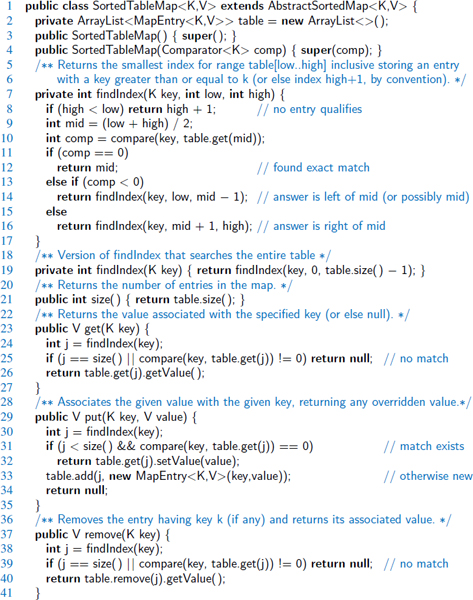
Code Fragment 10.11: An implementation of the SortedTableMap class. (Continues in Code Fragment 10.12.) The AbstractSorted Map base class (available online), provides the utility method, compare, based on a given comparator.

Code Fragment 10.12: An implementation of the SortedTableMap class (continued from Code Fragment 10.11).
Analysis
We conclude by analyzing the performance of our SortedTableMap implementation. A summary of the running times for all methods of the sorted map ADT (including the traditional map operations) is given in Table 10.3. It should be clear that the size, firstEntry, and lastEntry methods run in O(1) time, and that iterating the keys of the table in either direction can be performed in O(n) time.
The analysis for the various forms of search all depend on the fact that a binary search on a table with n entries runs in O(log n) time. This claim was originally shown as Proposition 5.2 in Section 5.2, and that analysis clearly applies to our findIndex method as well. We therefore claim an O(logn) worst-case running time for methods get, ceilingEntry, floorEntry, lowerEntry, and higherEntry. Each of these makes a single call to findIndex, followed by a constant number of additional steps to determine the appropriate answer based on the index. The analysis of subMap is a bit more interesting. It begins with a binary search to find the first item within the range (if any). After that, it executes a loop that takes O(1) time per iteration to gather subsequent values until reaching the end of the range. If there are s items reported in the range, the total running time is O(s + log n).
In contrast to the efficient search operations, update operations for a sorted table may take considerable time. Although binary search can help identify the index at which an update occurs, both insertions and deletions require, in the worst case, that linearly many existing elements be shifted in order to maintain the sorted order of the table. Specifically, the potential call to table.add from within put and table.remove from within remove lead to O(n) worst-case time. (See the discussion of corresponding operations of the ArrayList class in Section 7.2.)
In conclusion, sorted tables are primarily used in situations where we expect many searches but relatively few updates.
| Method | Running Time |
| size | O(1) |
| get | O(log n) |
| put | O(n); O(log n) if map has entry with given key |
| remove | O(n) |
| firstEntry, lastEntry | O(1) |
| ceilingEntry, floorEntry, lowerEntry, higherEntry | O(log n) |
| subMap | O(s + log n) where s items are reported |
| entrySet, keySet, values | O(n) |
Table 10.3: Performance of a sorted map, as implemented with SortedTableMap. We use n to denote the number of items in the map at the time the operation is performed. The space requirement is O(n).
10.3.2 Two Applications of Sorted Maps
In this section, we explore applications in which there is particular advantage to using a sorted map rather than a traditional (unsorted) map. To apply a sorted map, keys must come from a domain that is totally ordered. Furthermore, to take advantage of the inexact or range searches afforded by a sorted map, there should be some reason why nearby keys have relevance to a search.
Flight Databases
There are several websites on the Internet that allow users to perform queries on flight databases to find flights between various cities, typically with the intent to buy a ticket. To make a query, a user specifies origin and destination cities, a departure date, and a departure time. To support such queries, we can model the flight database as a map, where keys are Flight objects that contain fields corresponding to these four parameters. That is, a key is a tuple
k = (origin, destination, date, time).
Additional information about a flight, such as the flight number, the number of seats still available in first (F) and coach (Y) class, the flight duration, and the fare, can be stored in the value object.
Finding a requested flight is not simply a matter of finding an exact match for a requested query. Although a user typically wants to exactly match the origin and destination cities, he or she may have flexibility for the departure date, and certainly will have some flexibility for the departure time on a specific day. We can handle such a query by ordering our keys lexicographically. Then, an efficient implementation for a sorted map would be a good way to satisfy users' queries. For instance, given a user query key k, we could call ceilingEntry(k) to return the first flight between the desired cities, having a departure date and time matching the desired query or later. Better yet, with well-constructed keys, we could use subMap(k1, k2) to find all flights within a given range of times. For example, if k1 = (ORD, PVD, 05May, 09:30), and k2 = (ORD, PVD, 05May, 20:00), a respective call to subMap(k1, k2) might result in the following sequence of key-value pairs:

Maxima Sets
Life is full of trade-offs. We often have to trade off a desired performance measure against a corresponding cost. Suppose, for the sake of an example, we are interested in maintaining a database rating automobiles by their maximum speeds and their cost. We would like to allow someone with a certain amount of money to query our database to find the fastest car they can possibly afford.
We can model such a trade-off problem as this by using a key-value pair to model the two parameters that we are trading off, which in this case would be the pair (cost, speed) for each car. Notice that some cars are strictly better than other cars using this measure. For example, a car with cost-speed pair (30000, 100) is strictly better than a car with cost-speed pair (40000,90). At the same time, there are some cars that are not strictly dominated by another car. For example, a car with cost-speed pair (30000,100) may be better or worse than a car with cost-speed pair (40000,120), depending on how much money we have to spend. (See Figure 10.9.)

Figure 10.9: Illustrating the cost-performance trade-off with pairs represented by points in the plane. Notice that point p is strictly better than points c, d, and e, but may be better or worse than points a, b, f, g, and h, depending on the price we are willing to pay. Thus, if we were to add p to our set, we could remove the points c, d, and e, but not the others.
Formally, we say a cost-performance pair (a, b) dominates pair (c, d) ≠ (a, b) if a ≤ c and b ≥ d, that is, if the first pair has no greater cost and at least as good performance. A pair (a, b) is called a maximum pair if it is not dominated by any other pair. We are interested in maintaining the set of maxima of a collection of cost-performance pairs. That is, we would like to add new pairs to this collection (for example, when a new car is introduced), and to query this collection for a given dollar amount, d, to find the fastest car that costs no more than d dollars.
Maintaining a Maxima Set with a Sorted Map
We can store the set of maxima pairs in a sorted map so that the cost is the key field and performance (speed) is the value. We can then implement operations add(c, p), which adds a new cost-performance entry (c, p), and best(c), which returns the entry having best performance of those with cost at most c. Code Fragment 10.13 provides an implementation of such a CostPerformanceDatabase class.

Code Fragment 10.13: An implementation of a class maintaining a set of maximal cost-performance entries using a sorted map.
Unfortunately, if we implement the sorted map using the SortedTableMap class, the add behavior has O(n) worst-case running time. If, on the other hand, we implement the map using a skip list, which we next describe, we can perform best(c) queries in O(log n) expected time and add(c, p) updates in O((1 + r)log n) expected time, where r is the number of points removed.
10.4 Skip Lists
In Section 10.3.1, we saw that a sorted table will allow O(log n)-time searches via the binary search algorithm. Unfortunately, update operations on a sorted table have O(n) worst-case running time because of the need to shift elements. In Chapter 7 we demonstrated that linked lists support very efficient update operations, as long as the position within the list is identified. Unfortunately, we cannot perform fast searches on a standard linked list; for example, the binary search algorithm requires an efficient means for direct accessing an element of a sequence by index.
An interesting data structure for efficiently realizing the sorted map ADT is the skip list. Skip lists provide a clever compromise to efficiently support search and update operations; they are implemented as the java.util.ConcurrentSkipListMap class. A skip list S for a map M consists of a series of lists {S0, S1,..., Sh}. Each list Si stores a subset of the entries of M sorted by increasing keys, plus entries with two sentinel keys denoted −∞ and +∞, where −∞ is smaller than every possible key that can be inserted in M and +∞ is larger than every possible key that can be inserted in M. In addition, the lists in S satisfy the following:
- List S0 contains every entry of the map M (plus sentinels −∞ and +∞).
- For i = 1,..., h − 1, list Si contains (in addition to −∞ and +∞)a randomly generated subset of the entries in list Si−1.
- List Sh contains only −∞ and +∞.
An example of a skip list is shown in Figure 10.10. It is customary to visualize a skip list S with list S0 at the bottom and lists S1, ..., Sh above it. Also, we refer to h as the height of skip list S.
Intuitively, the lists are set up so that Si + 1 contains roughly alternate entries of Si. However, the halving of the number of entries from one list to the next is not enforced as an explicit property of skip lists; instead, randomization is used. As we shall see in the details of the insertion method, the entries in Si + 1 are chosen at random from the entries in Si by picking each entry from Si to also be in Si + 1 with probability 1/2. That is, in essence, we “flip a coin” for each entry in Si and place that entry in Si+1 if the coin comes up “heads.” Thus, we expect S1 to have about n/2 entries, S2 to have about n/4 entries, and, in general, Si to have about n/2i entries. As a consequence, we expect the height h of S to be about log n.

Figure 10.10: Example of a skip list storing 10 entries. For simplicity, we show only the entries' keys, not their associated values.
Functions that generate random-like numbers are built into most modern computers, because they are used extensively in computer games, cryptography, and computer simulations. Some functions, called pseudorandom number generators, generate such numbers, starting with an initial seed. (See discussion of the java.util.Random class in Section 3.1.3.) Other methods use hardware devices to extract “true” random numbers from nature. In any case, we will assume that our computer has access to numbers that are sufficiently random for our analysis.
An advantage of using randomization in data structure and algorithm design is that the structures and methods that result can be simple and efficient. The skip list has the same logarithmic time bounds for searching as is achieved by the binary search algorithm, yet it extends that performance to update methods when inserting or deleting entries. Nevertheless, the bounds are expected for the skip list, while binary search of a sorted table has a worst-case bound.
A skip list makes random choices in arranging its structure in such a way that search and update times are O(log n) on average, where n is the number of entries in the map. Interestingly, the notion of average time complexity used here does not depend on the probability distribution of the keys in the input. Instead, it depends on the use of a random-number generator in the implementation of the insertions to help decide where to place the new entry. The running time is averaged over all possible outcomes of the random numbers used when inserting entries.
As with the position abstraction used for lists and trees, we view a skip list as a two-dimensional collection of positions arranged horizontally into levels and vertically into towers. Each level is a list Si and each tower contains positions storing the same entry across consecutive lists. The positions in a skip list can be traversed using the following operations:
| next(p): | Returns the position following p on the same level. |
| prev(p): | Returns the position preceding p on the same level. |
| above(p): | Returns the position above p in the same tower. |
| below(p): | Returns the position below p in the same tower. |
We conventionally assume that these operations return null if the position requested does not exist. Without going into the details, we note that we can easily implement a skip list by means of a linked structure such that the individual traversal methods each take O(1) time, given a skip-list position p. Such a linked structure is essentially a collection of h doubly linked lists aligned at towers, which are also doubly linked lists.
10.4.1 Search and Update Operations in a Skip List
The skip-list structure affords simple map search and update algorithms. In fact, all of the skip-list search and update algorithms are based on an elegant SkipSearch method that takes a key k and finds the position p of the entry in list S0 that has the largest key less than or equal to k (which is possibly −∞).
Searching in a Skip List
Suppose we are given a search key k. We begin the SkipSearch method by setting a position variable p to the topmost, left position in the skip list S, called the start position of S. That is, the start position is the position of Sh storing the special entry with key −∞. We then perform the following steps (see Figure 10.11), where key(p) denotes the key of the entry at position p:
- If S.below(p) is null, then the search terminates—we are at the bottom and have located the entry in S with the largest key less than or equal to the search key k. Otherwise, we drop down to the next lower level in the present tower by setting p = S.below(p).
- Starting at position p, we move p forward until it is at the rightmost position on the present level such that key(p) ≤ k. We call this the scan forward step. Note that such a position always exists, since each level contains the keys and −∞. It may be that p remains where it started after we perform such a forward scan for this level.
- Return to step 1.

Figure 10.11: Example of a search in a skip list. The positions examined when searching for key 50 are highlighted.
We give a pseudocode description of the skip-list search algorithm, SkipSearch, in Code Fragment 10.14. Given this method, we perform the map operation get(k) by computing p = SkipSearch(k) and testing whether or not key(p) = k. If these two keys are equal, we return the associated value; otherwise, we return null.

Code Fragment 10.14: Algorithm to search a skip list S for key k. Variable s holds the start position of S.
As it turns out, the expected running time of algorithm SkipSearch on a skip list with n entries is O(log n). We postpone the justification of this fact, however, until after we discuss the implementation of the update methods for skip lists. Navigation starting at the position identified by SkipSearch(k) can be easily used to provide the additional forms of searches in the sorted map ADT (e.g., ceilingEntry, subMap).
Insertion in a Skip List
The execution of the map operation put(k, v) begins with a call to SkipSearch(k). This gives us the position p of the bottom-level entry with the largest key less than or equal to k (note that p may hold the special entry with key −∞). If key(p) = k, the associated value is overwritten with v. Otherwise, we need to create a new tower for entry (k, v). We insert (k, v) immediately after position p within S0. After inserting the new entry at the bottom level, we use randomization to decide the height of the tower for the new entry. We “flip” a coin, and if the flip comes up tails, then we stop here. Else (the flip comes up heads), we backtrack to the previous (next higher) level and insert (k, v) in this level at the appropriate position. We again flip a coin; if it comes up heads, we go to the next higher level and repeat. Thus, we continue to insert the new entry (k, v) in lists until we finally get a flip that comes up tails. We link together all the references to the new entry (k, v) created in this process to create its tower. A fair coin flip can be simulated with Java's built-in pseudorandom number generator java.util.Random by calling nextBoolean(), which returns true or false, each with probability 1/2.
We give the insertion algorithm for a skip list S in Code Fragment 10.15 and we illustrate it in Figure 10.12. The algorithm uses an insertAfterAbove(p, q, (k, v)) method that inserts a position storing the entry (k, v) after position p (on the same level as p) and above position q, returning the new position r (and setting internal references so that next, prev, above, and below methods will work correctly for p, q, and r). The expected running time of the insertion algorithm on a skip list with n entries is O(log n), as we show in Section 10.4.2.

Code Fragment 10.15: Insertion in a skip list of entry (k, v) We assume the skip list does not have an entry with key k. Method coinFlip() returns “heads” or “tails”, each with probability 1/2. Instance variables n, h, and s respectively hold the number of entries, the height, and the start node of the skip list.

Figure 10.12: Insertion of an entry with key 42 into the skip list of Figure 10.10 using method SkipInsert (Code Fragment 10.15). We assume that the random “coin flips” for the new entry came up heads three times in a row, followed by tails. The positions visited are highlighted in blue. The positions of the tower of the new entry (variable q) are drawn with thick lines, and the positions preceding them (variable p) are flagged.
Removal in a Skip List
Like the search and insertion algorithms, the removal algorithm for a skip list is quite simple. In fact, it is even easier than the insertion algorithm. To perform the map operation remove(k), we will begin by executing method SkipSearch (k). If the returned position p stores an entry with key different from k, we return null. Otherwise, we remove p and all the positions above p, which are easily accessed by using above operations to climb up the tower of this entry in S starting at position p. While removing levels of the tower, we reestablish links between the horizontal neighbors of each removed position. The removal algorithm is illustrated in Figure 10.13 and a detailed description of it is left as an exercise (R-10.24). As we show in the next subsection, the remove operation in a skip list with n entries has O(log n) expected running time.
Before we give this analysis, however, there are some minor improvements to the skip-list data structure we would like to discuss. First, we do not actually need to store references to values at the levels of the skip list above the bottom level, because all that is needed at these levels are references to keys. In fact, we can more efficiently represent a tower as a single object, storing the key-value pair, and maintaining j previous references and j next references if the tower reaches level Sj. Second, for the horizontal axes, it is possible to keep the list singly linked, storing only the next references. We can perform insertions and removals in strictly a top-down, scan-forward fashion. We explore the details of this optimization in Exercise C-10.55. Neither of these optimizations improve the asymptotic performance of skip lists by more than a constant factor, but these improvements can, nevertheless, be meaningful in practice. In fact, experimental evidence suggests that optimized skip lists are faster in practice than AVL trees and other balanced search trees, which are discussed in Chapter 11.

Figure 10.13: Removal of the entry with key 25 from the skip list of Figure 10.12. The positions visited after the search for the position of S0 holding the entry are highlighted in blue. The positions removed are drawn with dashed lines.
Maintaining the Topmost Level
A skip list S must maintain a reference to the start position (the topmost, leftmost position in S) as an instance variable, and must have a policy for any insertion that wishes to continue growing the tower for a new entry past the top level of S. There are two possible courses of action we can take, both of which have their merits.
One possibility is to restrict the top level, h, to be kept at some fixed value that is a function of n, the number of entries currently in the map (from the analysis we will see that ![]() is a reasonable choice, and picking
is a reasonable choice, and picking ![]() is even safer). Implementing this choice means that we must modify the insertion algorithm to stop inserting a new position once we reach the topmost level (unless
is even safer). Implementing this choice means that we must modify the insertion algorithm to stop inserting a new position once we reach the topmost level (unless ![]() , in which case we can now go at least one more level, since the bound on the height is increasing).
, in which case we can now go at least one more level, since the bound on the height is increasing).
The other possibility is to let an insertion continue growing a tower as long as heads keep getting returned from the random number generator. This is the approach taken by algorithm Skiplnsert of Code Fragment 10.15. As we show in the analysis of skip lists, the probability that an insertion will go to a level that is more than O(log n) is very low, so this design choice should also work.
Either choice will still result in the expected O(log n) time to perform search, insertion, and removal, as we will show in the next section.
10.4.2 Probabilistic Analysis of Skip Lists 
As we have shown above, skip lists provide a simple implementation of a sorted map. In terms of worst-case performance, however, skip lists are not a superior data structure. In fact, if we do not officially prevent an insertion from continuing significantly past the current highest level, then the insertion algorithm can go into what is almost an infinite loop (it is not actually an infinite loop, however, since the probability of having a fair coin repeatedly come up heads forever is 0). Moreover, we cannot infinitely add positions to a list without eventually running out of memory. In any case, if we terminate position insertion at the highest level h, then the worst-case running time for performing the get, put, and remove map operations in a skip list S with n entries and height h is O(n + h). This worst-case performance occurs when the tower of every entry reaches level h − 1, where h is the height of S. However, this event has very low probability. Judging from this worst case, we might conclude that the skip-list structure is strictly inferior to the other map implementations discussed earlier in this chapter. But this would not be a fair analysis, for this worst-case behavior is a gross overestimate.
Bounding the Height of a Skip List
Because the insertion step involves randomization, a more accurate analysis of skip lists involves a bit of probability. At first, this might seem like a major undertaking, for a complete and thorough probabilistic analysis could require deep mathematics (and, indeed, there are several such deep analyses that have appeared in data structures research literature). Fortunately, such an analysis is not necessary to understand the expected asymptotic behavior of skip lists. The informal and intuitive probabilistic analysis we give below uses only basic concepts of probability theory.
Let us begin by determining the expected value of the height h of a skip list S with n entries (assuming that we do not terminate insertions early). The probability that a given entry has a tower of height i ≥ 1 is equal to the probability of getting i consecutive heads when flipping a coin, that is, this probability is 1/2i. Hence, the probability Pi that level i has at least one position is at most
![]()
because the probability that any one of n different events occurs is at most the sum of the probabilities that each occurs.
The probability that the height h of S is larger than i is equal to the probability that level i has at least one position, that is, it is no more than Pi. This means that h is larger than, say, 3 log n with probability at most

For example, if n = 1000, this probability is a one-in-a-million long shot. More generally, given a constant c > 1, h is larger than clog n with probability at most 1/nc−1. That is, the probability that h is smaller than clog n is at least 1 − 1/nc−1. Thus, with high probability, the height h of S is O(log n).
Analyzing Search Time in a Skip List
Next, consider the running time of a search in skip list S, and recall that such a search involves two nested while loops. The inner loop performs a scan forward on a level of S as long as the next key is no greater than the search key k, and the outer loop drops down to the next level and repeats the scan forward iteration. Since the height h of S is O(log n) with high probability, the number of drop-down steps is O(log n) with high probability.
So we have yet to bound the number of scan-forward steps we make. Let ni be the number of keys examined while scanning forward at level i. Observe that, after the key at the starting position, each additional key examined in a scan-forward at level i cannot also belong to level i + 1. If any of these keys were on the previous level, we would have encountered them in the previous scan-forward step. Thus, the probability that any key is counted in ni is 1/2. Therefore, the expected value of n is exactly equal to the expected number of times we must flip a fair coin before it comes up heads. This expected value is 2. Hence, the expected amount of time spent scanning forward at any level i is O(1). Since S has O(log n) levels with high probability, a search in S takes expected time O(log n). By a similar analysis, we can show that the expected running time of an insertion or a removal is O(log n).
Space Usage in a Skip List
Finally, let us turn to the space requirement of a skip list S with n entries. As we observed above, the expected number of positions at level i is n/2i, which means that the expected total number of positions in S is

Using Proposition 4.5 on geometric summations, we have

Hence, the expected space requirement of S is O(n).
Table 10.4 summarizes the performance of a sorted map realized by a skip list.
| Method | Running Time |
| size, isEmpty | O(1) |
| get | O(log n) expected |
| put | O(log n) expected |
| remove | O(log n) expected |
| first Entry, lastEntry | O(1) |
| ceilingEntry, floorEntry lowerEntry,higherEntry | O(log n) expected |
| subMap | O(s + log n) expected, with s entries reported |
| entrySet, keySet, values | O(n) |
Table 10.4: Performance of a sorted map implemented with a skip list. We use n to denote the number of entries in the dictionary at the time the operation is performed. The expected space requirement is O(n).
10.5 Sets, Multisets, and Multimaps
We conclude this chapter by examining several additional abstractions that are closely related to the map ADT, and that can be implemented using data structures similar to those for a map.
- A set is an unordered collection of elements, without duplicates, that typically supports efficient membership tests. In essence, elements of a set are like keys of a map, but without any auxiliary values.
- A multiset (also known as a bag) is a set-like container that allows duplicates.
- A multimap is similar to a traditional map, in that it associates values with keys; however, in a multimap the same key can be mapped to multiple values. For example, the index of this book (page 714) maps a given term to one or more locations at which the term occurs elsewhere in the book.
10.5.1 The Set ADT
The Java Collections Framework defines the java.util.Set interface, which includes the following fundamental methods:
| add(e): | Adds the element e to S (if not already present). |
| remove(e): | Removes the element e from S (if it is present). |
| contains(e): | Returns whether e is an element of S. |
| iterator(): | Returns an iterator of the elements of S. |
There is also support for the traditional mathematical set operations of union, intersection, and subtraction of two sets S and T:

In the java.util.Set interface, these operations are provided through the following methods, if executed on a set S:
| addAll(T): | Updates S to also include all elements of set T, effectively replacing S by S∪T. |
| retainAll(T): | Updates S so that it only keeps those elements that are also elements of set T, effectively replacing S by S∩T. |
| removeAll(T): | Updates S by removing any of its elements that also occur in set T, effectively replacing S by S−T. |
The template method pattern can be applied to implement each of the methods addAll, retainAll, and removeAll using only calls to the more fundamental methods add, remove, contains, and iterator. In fact, the java.util.AbstractSet class provides such implementations. To demonstrate the technique, we could implement the addAll method in the context of a set class as follows:
public void addAll(Set<E> other) {
 for (E element : other)         // rely on iterator( ) method of other
   add(element);                 // duplicates will be ignored by add
}
The removeAll and retailAll methods can be implemented with similar techniques, although a bit more care is needed for retainAll, to avoid removing elements while iterating over the same set (see Exercise C-10.59). The efficiency of these methods for a concrete set implementation will depend on the underlying efficiency of the fundamental methods upon which they rely.
Sorted Sets
For the standard set abstraction, there is no explicit notion of keys being ordered; all that is assumed is that the equals method can detect equivalent elements.
If, however, elements come from a Comparable class (or a suitable Comparator object is provided), we can extend the notion of a set to define the sorted set ADT, including the following additional methods:
| first(): | Returns the smallest element in S. |
| last(): | Returns the largest element in S. |
| ceiling(e): | Returns the smallest element greater than or equal to e. |
| floor(e): | Returns the largest element less than or equal to e. |
| lower(e): | Returns the largest element strictly less than e. |
| higher(e): | Returns the smallest element strictly greater than e. |
| subSet(e1, e2): | Returns an iteration of all elements greater than or equal to e1, but strictly less than e2. |
| pollFirst(): | Returns and removes the smallest element in S. |
| pollLast(): | Returns and removes the largest element in S. |
In the Java Collection Framework, the above methods are included in a combination of the java.util.SortedSet and java.util.NavigableSet interfaces.
Implementing Sets
Although a set is a completely different abstraction than a map, the techniques used to implement the two can be quite similar. In effect, a set is simply a map in which (unique) keys do not have associated values.
Therefore, any data structure used to implement a map can be modified to implement the set ADT with similar performance guarantees. As a trivial adaption of a map, each set element can be stored as a key, and the null reference can be stored as an (irrelevant) value. Of course, such an implementation is unnecessarily wasteful; a more efficient set implementation should abandon the Entry composite and store set elements directly in a data structure.
The Java Collections Framework includes the following set implementations, mirroring similar data structures used for maps:
- java.util.HashSet provides an implementation of the (unordered) set ADT with a hash table.
- java.util.concurrent.ConcurrentSkipListSet provides an implementation of the sorted set ADT using a skip list.
- java.util.TreeSet provides an implementation of the sorted set ADT using a balanced search tree. (Search trees are the focus of Chapter 11.)
10.5.2 The Multiset ADT
Before discussing models for a multiset abstraction, we must carefully consider the notion of “duplicate” elements. Throughout the Java Collections Framework, objects are considered equivalent to each other based on the standard equals method (see Section 3.5). For example, keys of a map must be unique, but the notion of uniqueness allows distinct yet equivalent objects to be matched. This is important for many typical uses of maps. For example, when strings are used as keys, the instance of the string "October" that is used when inserting an entry may not be the same instance of "October" that is used when later retrieving the associated value. The call birthstones.get("October") will succeed in such a scenario because strings are considered equal to each other.
In the context of multisets, if we represent a collection that appears through the notion of equivalence as {a, a, a, a, b, c, c}, we must decide if we want a data structure to explicitly maintain each instance of a (because each might be distinct though equivalent), or just that there exist four occurrences. In either case, a multiset can be implemented by directly adapting a map. We can use one element from a group of equivalent occurrences as the key in a map, with the associated value either a secondary container containing all of the equivalent instances, or a count of the number of occurrences. Note that our word-frequency application in Section 10.1.2 uses just such a map, associating strings with counts.
The Java Collections Framework does not include any form of a multiset. However, implementations exist in several widely used, open source Java collections libraries. The Apache Commons defines Bag and SortedBag interfaces that correspond respectively to unsorted and sorted multisets. The Google Core Libraries for Java (named Guava) includes Multiset and SortedMultiset interfaces for these abstractions. Both of those libraries take the approach of modeling a multiset as a collection of elements having multiplicities, and both offer several concrete implementations using standard data structures. In formalizing the abstract data type, the Multiset interface of the Guava library includes the following behaviors (and more):
| add(e): | Adds a single occurrences of e to the multiset. |
| contains(e): | Returns true if the multiset contains an element equal to e. |
| count(e): | Returns the number of occurrences of e in the multiset. |
| remove(e): | Removes a single occurrence of e from the multiset. |
| remove(e, n): | Removes n occurrences of e from the multiset. |
| size(): | Returns the number of elements of the multiset (including duplicates). |
| iterator(): | Returns an iteration of all elements of the multiset (repeating those with multiplicity greater than one). |
The multiset ADT also includes the notion of an immutable Entry that represents an element and its count, and the SortedMultiset interface includes additional methods such as firstEntry and lastEntry.
10.5.3 The Multimap ADT
Like a map, a multimap stores entries that are key-value pairs (k, v), where k is the key and v is the value. Whereas a map insists that entries have unique keys, a multimap allows multiple entries to have the same key, much like an English dictionary, which allows multiple definitions for the same word. That is, we will allow a multimap to contain entries (k, v) and (k, v′) having the same key.
There are two standard approaches for representing a multimap as a variation of a traditional map. One is to redesign the underlying data structure to allow separate entries to be stored for pairs such as (k, v) and (k, v′). The other is to map key k to a secondary container of all values associated with that key (e.g., {v, v′}).
Much as it is missing a formal abstraction for a multiset, the Java Collections Framework does not include any multiset interface nor implementations. However, as we will soon demonstrate, it is easy to represent a multiset by adapting other collection classes that are included in the java.util package.
To formalize the multimap abstract data type, we consider a simplified version of the Multimap interface included in Google's Guava library. Among its methods are the following:
| get(k): | Returns a collection of all values associated with key k in the multimap. |
| put(k, v): | Adds a new entry to the multimap associating key k with value v, without overwriting any existing mappings for key k. |
| remove(k, v): | Removes an entry mapping key k to value v from the multimap (if one exists). |
| removeAll(k): | Removes all entries having key equal to k from the multimap. |
| size(): | Returns the number of entries of the multiset (including multiple associations). |
| entries(): | Returns a collection of all entries in the multimap. |
| keys(): | Returns a collection of keys for all entries in the multimap (including duplicates for keys with multiple bindings). |
| keySet(): | Returns a nonduplicative collection of keys in the multimap. |
| values(): | Returns a collection of values for all entries in the multimap. |
In Code Fragments 10.16 and 10.17, we provide an implementation of a class, HashMultimap, that uses a java.util.HashMap to map each key to a secondary ArrayList of all values that are associated with the key. For brevity, we omit the formality of defining a Multimap interface, and we provide the entries() method as the only form of iteration.

Code Fragment 10.16: An implementation of a multimap as an adaptation of classes from the java.util package. (Continues in Code Fragment 10.17.)

Code Fragment 10.17: An implementation of a multimap as an adaptation of classes from the java.util package. (Continued from Code Fragment 10.16.)
10.6 Exercises
Reinforcement
| R-10.1 | What is the worst-case running time for inserting n key-value pairs into an initially empty map M that is implemented with the UnsortedTableMap class? |
| R-10.2 | Reimplement the UnsortedTableMap class using the PositionalList class from Section 7.3 rather than an ArrayList. |
| R-10.3 | The use of null values in a map is problematic, as there is then no way to differentiate whether a null value returned by the call get(k) represents the legitimate value of an entry (k, null), or designates that key k was not found. The java.util.Map interface includes a boolean method, containsKey(k), that resolves any such ambiguity. Implement such a method for the UnsortedTableMap class. |
| R-10.4 | Which of the hash table collision-handling schemes could tolerate a load factor above 1 and which could not? |
| R-10.5 | What would be a good hash code for a vehicle identification number that is a string of numbers and letters of the form “9X9XX99X9XX999999,” where a “9” represents a digit and an “X” represents a letter? |
| R-10.6 | Draw the 11-entry hash table that results from using the hash function, h(i) = (3i + 5) mod 11, to hash the keys 12, 44, 13, 88, 23, 94, 11, 39, 20, 16, and 5, assuming collisions are handled by chaining. |
| R-10.7 | What is the result of the previous exercise, assuming collisions are handled by linear probing? |
| R-10.8 | Show the result of Exercise R-10.6, assuming collisions are handled by quadratic probing, up to the point where the method fails. |
| R-10.9 | What is the result of Exercise R-10.6 when collisions are handled by double hashing using the secondary hash function h′(k) = 7 − (k mod 7)? |
| R-10.10 | What is the worst-case time for putting n entries in an initially empty hash table, with collisions resolved by chaining? What is the best case? |
| R-10.11 | Show the result of rehashing the hash table shown in Figure 10.6 into a table of size 19 using the new hash function h(k) = 3k mod 17. |
| R-10.12 | Modify the Pair class from Code Fragment 2.17 on page 92 so that it provides a natural definition for both the equals() and hashCode() methods. |
| R-10.13 | Consider lines 31–33 of Code Fragment 10.8 in our implementation of the class ChainHashMap. We use the difference in the size of a secondary bucket before and after a call to bucket.remove(k) to update the variable n. If we replace those three lines with the following, does the class behave properly? Explain.
V answer = bucket.remove(k); if (answer != null) // value of removed entry n−−; // size has decreased |
| R-10.14 | Our AbstractHashMap class maintains a load factor λ ≤ 0.5. Reimplement that class to allow the user to specify the maximum load, and adjust the concrete subclasses accordingly. |
| R-10.15 | Give a pseudocode description of an insertion into a hash table that uses quadratic probing to resolve collisions, assuming we also use the trick of replacing deleted entries with a special “available” object. |
| R-10.16 | Modify our ProbeHashMap to use quadratic probing. |
| R-10.17 | Explain why a hash table is not suited to implement a sorted map. |
| R-10.18 | What is the worst-case asymptotic running time for performing n deletions from a SortedTableMap instance that initially contains 2n entries? |
| R-10.19 | Implement the containKey(k) method, as described in Exercise R-10.3, for the SortedTableClass. |
| R-10.20 | Describe how a sorted list implemented as a doubly linked list could be used to implement the sorted map ADT. |
| R-10.21 | Consider the following variant of the findlndex method of the SortedTableMap class, originally given in Code Fragment 10.11:
1 private int findIndex(K key, int low, int high) {
2   if (high < low) return high + 1;
3   int mid = (low + high) / 2;
4   if (compare(key, table.get(mid)) < 0)
5       return findlndex(key, low, mid − 1);
6   else
7      return findlndex(key, mid + 1, high);
8  }
Does this always produce the same result as the original version? Justify your answer. |
| R-10.22 | What is the expected running time of the methods for maintaining a maxima set if we insert n pairs such that each pair has lower cost and performance than one before it? What is contained in the sorted map at the end of this series of operations? What if each pair had a lower cost and higher performance than the one before it? |
| R-10.23 | Draw the result after performing the following series of operations on the skip list shown in Figure 10.13: remove(38), put(48, x), put(24, y), remove(55). Use an actual coin flip to generate random bits as needed (and report your sequence of flips). |
| R-10.24 | Give a pseudocode description of the remove map operation for a skip list. |
| R-10.25 | Give a description, in pseudocode, for implementing the removeAll method for the set ADT, using only the other fundamental methods of the set. |
| R-10.26 | Give a description, in pseudocode, for implementing the retainAll method for the set ADT, using only the other fundamental methods of the set. |
| R-10.27 | If we let n denote the size of set S, and m denote the size of set T, what would be the running time of the operation S.addAll(T), as implemented on page 446, if both sets were implemented as skip lists? |
| R-10.28 | If we let n denote the size of set S, and m denote the size of set T, what would be the running time of the operation S.addAll(T), as implemented on page 446, if both sets were implemented using hashing? |
| R-10.29 | If we let n denote the size of set S, and m denote the size of set T, what would be the running time of the operation S.removeAll(T) when both sets are implemented using hashing? |
| R-10.30 | If we let n denote the size of set S, and m denote the size of set T, what would be the running time of the operation S.retainAll(T) when both sets are implemented using hashing? |
| R-10.31 | What abstraction would you use to manage a database of friends' birthdays in order to support efficient queries such as “find all friends whose birthday is today” and “find the friend who will be the next to celebrate a birthday”? |
Creativity
| C-10.32 | For an ideal compression function, the capacity of the bucket array for a hash table should be a prime number. Therefore, we consider the problem of locating a prime number in a range [M, 2M]. Implement a method for finding such a prime by using the sieve algorithm. In this algorithm, we allocate a 2M cell boolean array A, such that cell i is associated with the integer i. We then initialize the array cells to all be “true” and we “mark off” all the cells that are multiples of 2, 3, 5, 7, and so on. This process can stop after it reaches a number larger than |
| C-10.33 | Consider the goal of adding entry (k, v) to a map only if there does not yet exist some other entry with key k. For a map M (without null values), this might be accomplished as follows.
if (M.get(k) == null)
   M.put(k, v);
While this accomplishes the goal, its efficiency is less than ideal, as time will be spent on the failed search during the get call, and again during the put call (which always begins by trying to locate an existing entry with the given key). To avoid this inefficiency, some map implementations support a custom method putlfAbsent(k, v) that accomplishes this goal. Given such an implementation of putlfAbsent for the UnsortedTableMap class. |
| C-10.34 | Repeat Exercise C-10.33 for the ChainHashMap class. |
| C-10.35 | Repeat Exercise C-10.33 for the ProbeHashMap class. |
| C-10.36 | Describe how to redesign the AbstractHashMap framework to include support for a method, containsKey, as described in Exercise R-10.3. |
| C-10.37 | Modify the ChainHashMap class in accordance with your design for the previous exercise. |
| C-10.38 | Modify the ProbeHashMap class in accordance with Exercise C-10.36. |
| C-10.39 | Redesign the AbstractHashMap class so that it halves the capacity of the table if the load factor falls below 0.25. Your solution must not involve any changes to the concrete ProbeHashMap and ChainHashMap classes. |
| C-10.40 | The java.util.HashMap class uses separate chaining, but without any explicit secondary structures. The table is an array of entries, and each entry has an additional next field that can reference another entry in that bucket. In this way, the entry instances can be threaded as a singly linked list. Reimplement our ChainHashMap class using such an approach. |
| C-10.41 | Describe how to perform a removal from a hash table that uses linear probing to resolve collisions where we do not use a special marker to represent deleted elements. That is, we must rearrange the contents so that it appears that the removed entry was never inserted in the first place. |
| C-10.42 | The quadratic probing strategy has a clustering problem related to the way it looks for open slots. Namely, when a collision occurs at bucket h(k), it checks buckets A[(h(k) + i2) mod N], for i = 1,2,...,N − 1.
|
| C-10.43 | Redesign our ProbeHashMap class so that the sequence of secondary probes for collision resolution can be more easily customized. Demonstrate your new design by providing separate concrete subclasses for linear probing and quadratic probing. |
| C-10.44 | The java.util.LinkedHashMap class is a subclass of the standard HashMap class that retains the expected O(1) performance for the primary map operations while guaranteeing that iterations report entries of the map according to first-in, first-out (FIFO) principle. That is, the key that has been in the map the longest is reported first. (The order is unaffected when the value for an existing key is changed.) Describe an algorithmic approach for achieving such performance. |
| C-10.45 | Develop a location-aware version of the UnsortedTableMap class so that an operation remove(e) for existing Entry e can be implemented in O(1) time. |
| C-10.46 | Repeat the previous exercise for the ProbeHashMap class. |
| C-10.47 | Repeat Exercise C-10.45 for the ChainHashMap class. |
| C-10.48 | Although keys in a map are distinct, the binary search algorithm can be applied in a more general setting in which an array stores possibly duplicative elements in nondecreasing order. Consider the goal of identifying the index of the leftmost element with key greater than or equal to given k. Does the findIndex method as given in Code Fragment 10.11 guarantee such a result? Does the findIndex method as given in Exercise R-10.21 guarantee such a result? Justify your answers. |
| C-10.49 | Suppose we are given two sorted search tables S and T, each with n entries (with S and T being implemented with arrays). Describe an O(log2 n)-time algorithm for finding the kth smallest key in the union of the keys from S and T (assuming no duplicates). |
| C-10.50 | Give an O(log n)-time solution for the previous problem. |
| C-10.51 | Give an alternative implementation of the SortedTableMap's entrySet method that creates a lazy iterator rather than a snapshot. (See Section 7.4.2 for discussion of iterators.) |
| C-10.52 | Repeat the previous exercise for the ChainHashMap class. |
| C-10.53 | Repeat Exercise C-10.51 for the ProbeHashMap class. |
| C-10.54 | Given a database D of n cost-performance pairs (c, p), describe an algorithm for finding the maxima pairs of C in O(nlog n) time. |
| C-10.55 | Show that the methods above(p) and before(p) are not actually needed to efficiently implement a map using a skip list. That is, we can implement insertions and deletions in a skip list using a strictly top-down, scan-forward approach, without ever using the above or before methods. (Hint: In the insertion algorithm, first repeatedly flip the coin to determine the level where you should start inserting the new entry.) |
| C-10.56 | Describe how to modify the skip-list data structure to support the method median(), which returns the position of the element in the “bottom” list S0 at index |
| C-10.57 | Describe how to modify a skip-list representation so that index-based operations, such as retrieving the entry at index j, can be performed in O(log n) expected time. |
| C-10.58 | Suppose that each row of an n × n array A consists of 1's and 0's such that, in any row of A, all the 1's come before any 0's in that row. Assuming A is already in memory, describe a method running in O(nlog n) time (not O(n2) time) for counting the number of 1's in A. |
| C-10.59 | Give a concrete implementation of the retainAll method for the set ADT, using only the other fundamental methods of the set. You are to assume that the underlying set implementation uses fail-fast iterators (see Section 7.4.2). |
| C-10.60 | Consider sets whose elements are integers in the range [0, N − 1]. A popular scheme for representing a set A of this type is by means of a boolean array, B, where we say that x is in A if and only if B[x] = true. Since each cell of B can be represented with a single bit, B is sometimes referred to as a bit vector. Describe and analyze efficient algorithms for performing the methods of the set ADT assuming this representation. |
| C-10.61 | An inverted file is a critical data structure for implementing applications such an index of a book or a search engine. Given a document D, which can be viewed as an unordered, numbered list of words, an inverted file is an ordered list of words, L, such that, for each word w in L, we store the indices of the places in D where w appears. Design an efficient algorithm for constructing L from D. |
| C-10.62 | The operation get(k) for our multimap ADT is responsible for returning a collection of all values currently associated with key k. Design a variation of binary search for performing this operation on a sorted search table that includes duplicates, and show that it runs in time O(s + log n), where n is the number of elements in the dictionary and s is the number of entries with given key k. |
| C-10.63 | Describe an efficient multimap structure for storing n entries that have an associated set of r < n keys that come from a total order. That is, the set of keys is smaller than the number of entries. Your structure should perform operation getAll in O(logr + s) expected time, where s is the number of entries returned, operation entrySet() in O(n) time, and the remaining operations of the multimap ADT in O(log r) expected time. |
| C-10.64 | Describe an efficient multimap structure for storing n entries whose r < n keys have distinct hash codes. Your structure should perform operation getAll in O(1 + s) expected time, where s is the number of entries returned, operation entrySet() in O(n) time, and the remaining operations of the multimap ADT in O(1) expected time. |
Projects
Chapter Notes
Hashing is a well-studied technique. The reader interested in further study is encouraged to explore the book by Knuth [61], as well as the book by Vitter and Chen [92]. The denial-of-service vulnerability exploiting the worst-case performance of hash tables was first described by Crosby and Wallach [27], and later demonstrated by Klink and Walde [58]. The remedy adopted by the OpenJDK team for Java is described in [76].
Skip lists were introduced by Pugh [80]. Our analysis of skip lists is a simplification of a presentation given by Motwani and Raghavan [75]. For a more in-depth analysis of skip lists, please see the various research papers on skip lists that have appeared in the data structures literature [56, 77, 78]. Exercise C-10.42 was contributed by James Lee.
*We use a star (![]() ) to indicate sections containing material more advanced than the material in the rest of the chapter; this material can be considered optional in a first reading.
) to indicate sections containing material more advanced than the material in the rest of the chapter; this material can be considered optional in a first reading.