
Chapter
8
Trees

Contents
8.1.1 Tree Definitions and Properties
8.1.2 The Tree Abstract Data Type
8.1.3 Computing Depth and Height
8.2.1 The Binary Tree Abstract Data Type
8.2.2 Properties of Binary Trees
8.3.1 Linked Structure for Binary Trees
8.3.2 Array-Based Representation of a Binary Tree
8.3.3 Linked Structure for General Trees
8.4.1 Preorder and Postorder Traversals of General Trees
8.4.2 Breadth-First Tree Traversal
8.4.3 Inorder Traversal of a Binary Tree
8.4.4 Implementing Tree Traversals in Java
8.1 General Trees
Productivity experts say that breakthroughs come by thinking “nonlinearly.” In this chapter, we will discuss one of the most important nonlinear data structures in computing—trees. Tree structures are indeed a breakthrough in data organization, for they allow us to implement a host of algorithms much faster than when using linear data structures, such as arrays or linked lists. Trees also provide a natural organization for data, and consequently have become ubiquitous structures in file systems, graphical user interfaces, databases, websites, and many other computer systems.
It is not always clear what productivity experts mean by “nonlinear” thinking, but when we say that trees are “nonlinear,” we are referring to an organizational relationship that is richer than the simple “before” and “after” relationships between objects in sequences. The relationships in a tree are hierarchical, with some objects being “above” and some “below” others. Actually, the main terminology for tree data structures comes from family trees, with the terms “parent,” “child,” “ancestor,” and “descendant” being the most common words used to describe relationships. We show an example of a family tree in Figure 8.1.

Figure 8.1: A family tree showing some descendants of Abraham, as recorded in Genesis, chapters 25–36.
8.1.1 Tree Definitions and Properties
A tree is an abstract data type that stores elements hierarchically. With the exception of the top element, each element in a tree has a parent element and zero or more children elements. A tree is usually visualized by placing elements inside ovals or rectangles, and by drawing the connections between parents and children with straight lines. (See Figure 8.2.) We typically call the top element the root of the tree, but it is drawn as the highest element, with the other elements being connected below (just the opposite of a botanical tree).

Figure 8.2: A tree with 17 nodes representing the organization of a fictitious corporation. The root stores Electronics R'Us. The children of the root store R&D, Sales, Purchasing, and Manufacturing. The internal nodes store Sales, International, Overseas, Electronics R'Us, and Manufacturing.
Formal Tree Definition
Formally, we define a tree T as a set of nodes storing elements such that the nodes have a parent-child relationship that satisfies the following properties:
- If T is nonempty, it has a special node, called the root of T, that has no parent.
- Each node v of T different from the root has a unique parent node w; every node with parent w is a child of w.
Note that according to our definition, a tree can be empty, meaning that it does not have any nodes. This convention also allows us to define a tree recursively such that a tree T is either empty or consists of a node r, called the root of T, and a (possibly empty) set of subtrees whose roots are the children of r.
Other Node Relationships
Two nodes that are children of the same parent are siblings. A node v is external if v has no children. A node v is internal if it has one or more children. External nodes are also known as leaves.
Example 8.1: In Section 5.1.4, we discussed the hierarchical relationship between files and directories in a computer's file system, although at the time we did not emphasize the nomenclature of a file system as a tree. In Figure 8.3, we revisit an earlier example. We see that the internal nodes of the tree are associated with directories and the leaves are associated with regular files. In the Unix and Linux operating systems, the root of the tree is appropriately called the “root directory,” and is represented by the symbol “/”.
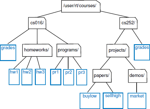
Figure 8.3: Tree representing a portion of a file system.
A node u is an ancestor of a node v if u = v or u is an ancestor of the parent of v. Conversely, we say that a node v is a descendant of a node u if u is an ancestor of v. For example, in Figure 8.3, cs252/ is an ancestor of papers/, and pr3 is a descendant of cs016/. The subtree of T rooted at a node v is the tree consisting of all the descendants of v in T (including v itself). In Figure 8.3, the subtree rooted at cs016/ consists of the nodes cs016/, grades, homeworks/, programs/, hwl, hw2, hw3, prl, pr2, and pr3.
Edges and Paths in Trees
An edge of tree T is a pair of nodes (u, v) such that u is the parent of v, or vice versa. A path of T is a sequence of nodes such that any two consecutive nodes in the sequence form an edge. For example, the tree in Figure 8.3 contains the path (cs252/, projects/, demos/, market).
Ordered Trees
A tree is ordered if there is a meaningful linear order among the children of each node; that is, we purposefully identify the children of a node as being the first, second, third, and so on. Such an order is usually visualized by arranging siblings left to right, according to their order.
Example 8.2: The components of a structured document, such as a book, are hierarchically organized as a tree whose internal nodes are parts, chapters, and sections, and whose leaves are paragraphs, tables, figures, and so on. (See Figure 8.4.) The root of the tree corresponds to the book itself. We could, in fact, consider expanding the tree further to show paragraphs consisting of sentences, sentences consisting of words, and words consisting of characters. Such a tree is an example of an ordered tree, because there is a well-defined order among the children of each node.

Figure 8.4: An ordered tree associated with a book.
Let's look back at the other examples of trees that we have described thus far, and consider whether the order of children is significant. A family tree that describes generational relationships, as in Figure 8.1, is often modeled as an ordered tree, with siblings ordered according to their birth.
In contrast, an organizational chart for a company, as in Figure 8.2, is typically considered an unordered tree. Likewise, when using a tree to describe an inheritance hierarchy, as in Figure 2.7, there is no particular significance to the order among the subclasses of a parent class. Finally, we consider the use of a tree in modeling a computer's file system, as in Figure 8.3. Although an operating system often displays entries of a directory in a particular order (e.g., alphabetical, chronological), such an order is not typically inherent to the file system's representation.
8.1.2 The Tree Abstract Data Type
As we did with positional lists in Section 7.3, we define a tree ADT using the concept of a position as an abstraction for a node of a tree. An element is stored at each position, and positions satisfy parent-child relationships that define the tree structure. A position object for a tree supports the method:
| getElement(): | Returns the element stored at this position. |
The tree ADT then supports the following accessor methods, allowing a user to navigate the various positions of a tree T:
| root(): | Returns the position of the root of the tree (or null if empty). |
| parent(p): | Returns the position of the parent of position p (or null if p is the root). |
| children(p): | Returns an iterable collection containing the children of position p (if any). |
| numChildren(p): | Returns the number of children of position p. |
If a tree T is ordered, then children(p) reports the children of p in order.
In addition to the above fundamental accessor methods, a tree supports the following query methods:
| isInternal(p): | Returns true if position p has at least one child. |
| isExternal(p): | Returns true if position p does not have any children. |
| isRoot(p): | Returns true if position p is the root of the tree. |
These methods make programming with trees easier and more readable, since we can use them in the conditionals of if statements and while loops.
Trees support a number of more general methods, unrelated to the specific structure of the tree. These include:
| size(): | Returns the number of positions (and hence elements) that are contained in the tree. |
| isEmpty(): | Returns true if the tree does not contain any positions (and thus no elements). |
| iterator(): | Returns an iterator for all elements in the tree (so that the tree itself is Iterable). |
| positions(): | Returns an iterable collection of all positions of the tree. |
If an invalid position is sent as a parameter to any method of a tree, then an IllegalArgumentException is thrown.
We do not define any methods for creating or modifying trees at this point. We prefer to describe different tree update methods in conjunction with specific implementations of the tree interface, and specific applications of trees.
A Tree Interface in Java
In Code Fragment 8.1, we formalize the Tree ADT by defining the Tree interface in Java. We rely upon the same definition of the Position interface as introduced for positional lists in Section 7.3.2. Note well that we declare the Tree interface to formally extend Java's Iterable interface (and we include a declaration of the required iterator() method).
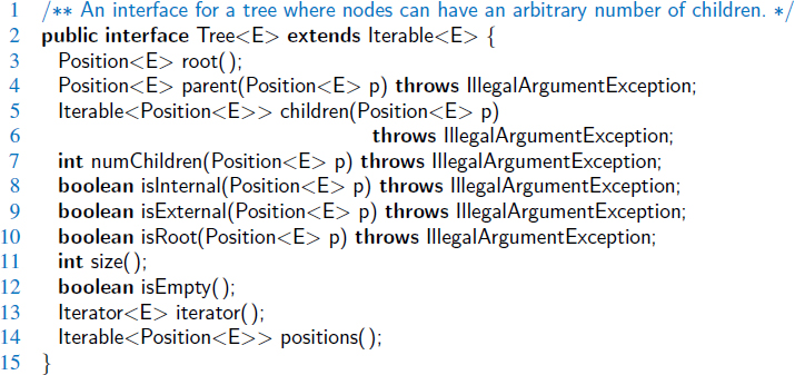
Code Fragment 8.1: Definition of the Tree interface.
An AbstractTree Base Class in Java
In Section 2.3, we discussed the role of interfaces and abstract classes in Java. While an interface is a type definition that includes public declarations of various methods, an interface cannot include definitions for any of those methods. In contrast, an abstract class may define concrete implementations for some of its methods, while leaving other abstract methods without definition.
An abstract class is designed to serve as a base class, through inheritance, for one or more concrete implementations of an interface. When some of the functionality of an interface is implemented in an abstract class, less work remains to complete a concrete implementation. The standard Java libraries include many such abstract classes, including several within the Java Collections Framework. To make their purpose clear, those classes are conventionally named beginning with the word Abstract. For example, there is an AbstractCollection class that implements some of the functionality of the Collection interface, an AbstractQueue class that implements some of the functionality of the Queue interface, and an AbstractList class that implements some of the functionality of the List interface.
In the case of our Tree interface, we will define an AbstractTree base class, demonstrating how many tree-based algorithms can be described independently of the low-level representation of a tree data structure. In fact, if a concrete implementation provides three fundamental methods—root(), parent(p), and children(p)—all other behaviors of the Tree interface can be derived within the AbstractTree base class.
Code Fragment 8.2 presents an initial implementation of an AbstractTree base class that provides the most trivial methods of the Tree interface. We will defer until Section 8.4 a discussion of general tree-traversal algorithms that can be used to produced the positions() iteration within the AbstractTree class. As with our positional list ADT in Chapter 7, the iteration of positions of the tree can easily be adapted to produce an iteration of the elements of a tree, or even to determine the size of a tree (although our concrete tree implementations will provide more direct means for reporting the size).

Code Fragment 8.2: An initial implementation of the AbstractTree base class. (We add additional functionality to this class as the chapter continues.)
8.1.3 Computing Depth and Height
Let p be a position within tree T. The depth of p is the number of ancestors of p, other than p itself. For example, in the tree of Figure 8.2, the node storing International has depth 2. Note that this definition implies that the depth of the root of T is 0. The depth of p can also be recursively defined as follows:
- If p is the root, then the depth of p is 0.
- Otherwise, the depth of p is one plus the depth of the parent of p.
Based on this definition, we present a simple recursive algorithm, depth, in Code Fragment 8.3, for computing the depth of a position p in tree T. This method calls itself recursively on the parent of p, and adds 1 to the value returned.
The running time of depth(p) for position p is O(dp + 1), where dp denotes the depth of p in the tree, because the algorithm performs a constant-time recursive step for each ancestor of p. Thus, algorithm depth(p) runs in O(n) worst-case time, where n is the total number of positions of T, because a position of T may have depth n − 1 if all nodes form a single branch. Although such a running time is a function of the input size, it is more informative to characterize the running time in terms of the parameter dp, as this parameter may be much smaller than n.

Code Fragment 8.3: Method depth, as implemented within the AbstractTree class.
Height
We next define the height of a tree to be equal to the maximum of the depths of its positions (or zero, if the tree is empty). For example, the tree of Figure 8.2 has height 4, as the node storing Africa (and its siblings) has depth 4. It is easy to see that the position with maximum depth must be a leaf.
In Code Fragment 8.4, we present a method that computes the height of a tree based on this definition. Unfortunately, such an approach is not very efficient, and so name the algorithm heightBad and declare it as a private method of the AbstractTree class (so that it cannot be used by others).

Code Fragment 8.4: Method heightBad of the AbstractTree class. Note that this method calls the depth method from Code Fragment 8.3.
Although we have not yet defined the positions() method, we will see that it can be implemented such that the entire iteration runs in O(n) time, where n is the number of positions of T. Because heightBad calls algorithm depth(p) on each leaf of T, its running time is O(n + Σp∈L(dp + 1)), where L is the set of leaf positions of T. In the worst case, the sum Σp∈L(dp + 1) is proportional to n2. (See Exercise C-8.31.) Thus, algorithm heightBad runs in O(n2) worst-case time.
We can compute the height of a tree more efficiently, in O(n) worst-case time, by considering a recursive definition. To do this, we will parameterize a function based on a position within the tree, and calculate the height of the subtree rooted at that position. Formally, we define the height of a position p in a tree T as follows:
- If p is a leaf, then the height of p is 0.
- Otherwise, the height of p is one more than the maximum of the heights of p's children.
The following proposition relates our original definition of the height of a tree to the height of the root position using this recursive formula.
Proposition 8.3: The height of the root of a nonempty tree T, according to the recursive definition, equals the maximum depth among all leaves of tree T.
We leave the justification of this proposition as Exercise R-8.3.
An implementation of a recursive algorithm to compute the height of a subtree rooted at a given position p is presented in Code Fragment 8.5. The overall height of a nonempty tree can be computed by sending the root of the tree as a parameter.
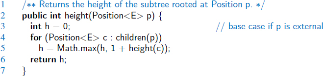
Code Fragment 8.5: Method height for computing the height of a subtree rooted at a position p of an AbstractTree.
It is important to understand why method height is more efficient than method heightBad. The algorithm is recursive, and it progresses in a top-down fashion. If the method is initially called on the root of T, it will eventually be called once for each position of T. This is because the root eventually invokes the recursion on each of its children, which in turn invokes the recursion on each of their children, and so on.
We can determine the running time of the recursive height algorithm by summing, over all the positions, the amount of time spent on the nonrecursive part of each call. (Review Section 5.2 for analyses of recursive processes.) In our implementation, there is a constant amount of work per position, plus the overhead of computing the maximum over the iteration of children. Although we do not yet have a concrete implementation of children(p), we assume that such an iteration is executed in O(cp + 1) time, where cp denotes the number of children of p. Algorithm height(p) spends O(cp +1) time at each position p to compute the maximum, and its overall running time is O(Σp(cp + 1)) = O(n + Σpcp). In order to complete the analysis, we make use of the following property.
Proposition 8.4: Let T be a tree with n positions, and let cp denote the number of children of a position p of T. Then, summing over the positions of T, Σpcp = n − 1.
Justification: Each position of T, with the exception of the root, is a child of another position, and thus contributes one unit to the above sum.
By Proposition 8.4, the running time of algorithm height, when called on the root of T, is O(n), where n is the number of positions of T.
8.2 Binary Trees
A binary tree is an ordered tree with the following properties:
- Every node has at most two children.
- Each child node is labeled as being either a left child or a right child.
- A left child precedes a right child in the order of children of a node.
The subtree rooted at a left or right child of an internal node v is called a left subtree or right subtree, respectively, of v. A binary tree is proper if each node has either zero or two children. Some people also refer to such trees as being full binary trees. Thus, in a proper binary tree, every internal node has exactly two children. A binary tree that is not proper is improper.
Example 8.5: An important class of binary trees arises in contexts where we wish to represent a number of different outcomes that can result from answering a series of yes-or-no questions. Each internal node is associated with a question. Starting at the root, we go to the left or right child of the current node, depending on whether the answer to the question is “Yes” or “No.” With each decision, we follow an edge from a parent to a child, eventually tracing a path in the tree from the root to a leaf. Such binary trees are known as decision trees, because a leaf position p in such a tree represents a decision of what to do if the questions associated with p's ancestors are answered in a way that leads to p. A decision tree is a proper binary tree. Figure 8.5 illustrates a decision tree that provides recommendations to a prospective investor.

Figure 8.5: A decision tree providing investment advice.
Example 8.6: An arithmetic expression can be represented by a binary tree whose leaves are associated with variables or constants, and whose internal nodes are associated with one of the operators +, −, *, and /, as demonstrated in Figure 8.6. Each node in such a tree has a value associated with it.
- If a node is leaf, then its value is that of its variable or constant.
- If a node is internal, then its value is defined by applying its operation to the values of its children.
A typical arithmetic expression tree is a proper binary tree, since each operator +, −, *, and / takes exactly two operands. Of course, if we were to allow unary operators, like negation (−), as in “−x,” then we could have an improper binary tree.

Figure 8.6: A binary tree representing an arithmetic expression. This tree represents the expression ((((3 + 1) * 3)/((9 − 5) + 2)) − ((3 * (7 − 4)) + 6)). The value associated with the internal node labeled “/” is 2.
A Recursive Binary Tree Definition
Incidentally, we can also define a binary tree in a recursive way. In that case, a binary tree is either:
- An empty tree.
- A nonempty tree having a root node r, which stores an element, and two binary trees that are respectively the left and right subtrees of r. We note that one or both of those subtrees can be empty by this definition.
8.2.1 The Binary Tree Abstract Data Type
As an abstract data type, a binary tree is a specialization of a tree that supports three additional accessor methods:
| left(p): | Returns the position of the left child of p (or null if p has no left child). |
| right(p): | Returns the position of the right child of p (or null if p has no right child). |
| sibling(p): | Returns the position of the sibling of p (or null if p has no sibling). |
Just as in Section 8.1.2 for the tree ADT, we do not define specialized update methods for binary trees here. Instead, we will consider some possible update methods when we describe specific implementations and applications of binary trees.
Defining a BinaryTree Interface
Code Fragment 8.6 formalizes the binary tree ADT by defining a BinaryTree interface in Java. This interface extends the Tree interface that was given in Section 8.1.2 to add the three new behaviors. In this way, a binary tree is expected to support all the functionality that was defined for general trees (e.g., root, isExternal, parent), and the new behaviors left, right, and sibling.

Code Fragment 8.6: A BinaryTree interface that extends the Tree interface from Code Fragment 8.1.
Defining an AbstractBinaryTree Base Class
We continue our use of abstract base classes to promote greater reusability within our code. The AbstractBinaryTree class, presented in Code Fragment 8.7, inherits from the AbstractTree class from Section 8.1.2. It provides additional concrete methods that can be derived from the newly declared left and right methods (which remain abstract).
The new sibling method is derived from a combination of left, right, and parent. Typically, we identify the sibling of a position p as the “other” child of p's parent. However, p does not have a sibling if it is the root, or if it is the only child of its parent.
We can also use the presumed left and right methods to provide concrete implementations of the numChildren and children methods, which are part of the original Tree interface. Using the terminology of Section 7.4, the implementation of the children method relies on producing a snapshot. We create an empty java.util.ArrayList, which qualifies as being an iterable container, and then add any children that exist, ordered so that a left child is reported before a right child.

Code Fragment 8.7: An AbstractBinaryTree class that extends the AbstractTree class of Code Fragment 8.2 and implements the BinaryTree interface of Code Fragment 8.6.
8.2.2 Properties of Binary Trees
Binary trees have several interesting properties dealing with relationships between their heights and number of nodes. We denote the set of all nodes of a tree T at the same depth d as level d of T. In a binary tree, level 0 has at most one node (the root), level 1 has at most two nodes (the children of the root), level 2 has at most four nodes, and so on. (See Figure 8.7.) In general, level d has at most 2d nodes.

Figure 8.7: Maximum number of nodes in the levels of a binary tree.
We can see that the maximum number of nodes on the levels of a binary tree grows exponentially as we go down the tree. From this simple observation, we can derive the following properties relating the height of a binary tree T with its number of nodes. A detailed justification of these properties is left as Exercise R-8.8.
Proposition 8.7: Let T be a nonempty binary tree, and let n, nE, nI, and h denote the number of nodes, number of external nodes, number of internal nodes, and height of T, respectively. Then T has the following properties:
- h + 1 ≤ n ≤ 2h+1 − 1
- 1 ≤ nE ≤ 2h
- h ≤ nI ≤ 2h − 1
- log(n + 1) − 1 ≤ h ≤ n − 1
Also, if T is proper, then T has the following properties:
- 2h + 1 ≤ n ≤ 2h+1 − 1
- h + 1 ≤ nE ≤ 2h
- h ≤ nI ≤ 2h − 1
- log(n + 1) − 1 ≤ h ≤ (n − 1)/2
Relating Internal Nodes to External Nodes in a Proper Binary Tree
In addition to the earlier binary tree properties, the following relationship exists between the number of internal nodes and external nodes in a proper binary tree.
Proposition 8.8: In a nonempty proper binary tree T, with nE external nodes and nI internal nodes, we have nE = nI + 1.
Justification: We justify this proposition by removing nodes from T and dividing them up into two “piles,” an internal-node pile and an external-node pile, until T becomes empty. The piles are initially empty. By the end, we will show that the external-node pile has one more node than the internal-node pile. We consider two cases:
Case 1: If T has only one node v, we remove v and place it on the external-node pile. Thus, the external-node pile has one node and the internal-node pile is empty.
Case 2: Otherwise (T has more than one node), we remove from T an (arbitrary) external node w and its parent v, which is an internal node. We place w on the external-node pile and v on the internal-node pile. If v has a parent u, then we reconnect u with the former sibling z of w, as shown in Figure 8.8. This operation, removes one internal node and one external node, and leaves the tree being a proper binary tree.
Repeating this operation, we eventually are left with a final tree consisting of a single node. Note that the same number of external and internal nodes have been removed and placed on their respective piles by the sequence of operations leading to this final tree. Now, we remove the node of the final tree and we place it on the external-node pile. Thus, the external-node pile has one more node than the internal-node pile.

Figure 8.8: Operation that removes an external node and its parent node, used in the justification of Proposition 8.8.
Note that the above relationship does not hold, in general, for improper binary trees and nonbinary trees, although there are other interesting relationships that do hold. (See Exercises C-8.30 through C-8.32.)
8.3 Implementing Trees
The AbstractTree and AbstractBinaryTree classes that we have defined thus far in this chapter are both abstract base classes. Although they provide a great deal of support, neither of them can be directly instantiated. We have not yet defined key implementation details for how a tree will be represented internally, and how we can effectively navigate between parents and children.
There are several choices for the internal representation of trees. We describe the most common representations in this section. We begin with the case of a binary tree, since its shape is more strictly defined.
8.3.1 Linked Structure for Binary Trees
A natural way to realize a binary tree T is to use a linked structure, with a node (see Figure 8.9a) that maintains references to the element stored at a position p and to the nodes associated with the children and parent of p. If p is the root of T, then the parent field of p is null. Likewise, if p does not have a left child (respectively, right child), the associated field is null. The tree itself maintains an instance variable storing a reference to the root node (if any), and a variable, called size, that represents the overall number of nodes of T. We show such a linked structure representation of a binary tree in Figure 8.9b.

Figure 8.9: A linked structure for representing: (a) a single node; (b) a binary tree.
Operations for Updating a Linked Binary Tree
The Tree and BinaryTree interfaces define a variety of methods for inspecting an existing tree, yet they do not declare any update methods. Presuming that a newly constructed tree is empty, we would like to have means for changing the structure of content of a tree.
Although the principle of encapsulation suggests that the outward behaviors of an abstract data type need not depend on the internal representation, the efficiency of the operations depends greatly upon the representation. We therefore prefer to have each concrete implementation of a tree class support the most suitable behaviors for updating a tree. In the case of a linked binary tree, we suggest that the following update methods be supported:
| add Root(e): | Creates a root for an empty tree, storing e as the element, and returns the position of that root; an error occurs if the tree is not empty. |
| addLeft(p, e): | Creates a left child of position p, storing element e, and returns the position of the new node; an error occurs if p already has a left child. |
| addRight(p, e): | Creates aright child of position p, storing element e, and returns the position of the new node; an error occurs if p already has a right child. |
| set(p, e): | Replaces the element stored at position p with element e, and returns the previously stored element. |
| attach(p, T1, T2): | Attaches the internal structure of trees T1 and T2 as the respective left and right subtrees of leaf position p and resets T1 and T2 to empty trees; an error condition occurs if p is not a leaf. |
| remove(p): | Removes the node at position p, replacing it with its child (if any), and returns the element that had been stored at p; an error occurs if p has two children. |
We have specifically chosen this collection of operations because each can be implemented in O(1) worst-case time with our linked representation. The most complex of these are attach and remove, due to the case analyses involving the various parent-child relationships and boundary conditions, yet there remains only a constant number of operations to perform. (The implementation of both methods could be greatly simplified if we used a tree representation with a sentinel node, akin to our treatment of positional lists; see Exercise C-8.38.)
Java Implementation of a Linked Binary Tree Structure
We now present a concrete implementation of a LinkedBinaryTree class that implements the binary tree ADT, and supports the update methods described on the previous page. The new class formally extends the AbstractBinaryTree base class, inheriting several concrete implementations of methods from that class (as well as the formal designation that it implements the BinaryTree interface).
The low-level details of our linked tree implementation are reminiscent of techniques used when implementing the LinkedPositionalList class in Section 7.3.3. We define a nonpublic nested Node class to represent a node, and to serve as a Position for the public interface. As was portrayed in Figure 8.9, a node maintains a reference to an element, as well as references to its parent, its left child, and its right child (any of which might be null). The tree instance maintains a reference to the root node (possibly null), and a count of the number of nodes in the tree.
We also provide a validate utility that is called anytime a Position is received as a parameter, to ensure that it is a valid node. In the case of a linked tree, we adopt a convention in which we set a node's parent pointer to itself when it is removed from a tree, so that we can later recognize it as an invalid position.
The entire LinkedBinaryTree class is presented in Code Fragments 8.8–8.11. We provide the following guide to that code:
- Code Fragment 8.8 contains the definition of the nested Node class, which implements the Position interface. It also defines a method, createNode, that returns a new node instance. Such a design uses what is known as the factory method pattern, allowing us to later subclass our tree in order to use a specialized node type. (See Section 11.2.1.) Code Fragment 8.8 concludes with the declaration of the instance variables of the outer LinkedBinaryTree class and its constructor.
- Code Fragment 8.9 includes the protected validate(p) method, followed by the accessors size, root, left, and right. We note that all other methods of the Tree and BinaryTree interfaces are derived from these four concrete methods, via the AbstractTree and AbstractBinaryTree base classes.
- Code Fragments 8.10 and 8.11 provide the six update methods for a linked binary tree, as described on the preceding page. We note that the three methods—addRoot, addLeft, and addRight—each rely on use of the factory method, createNode, to produce a new node instance.
The remove method, given at the end of Code Fragment 8.11, intentionally sets the parent field of a deleted node to refer to itself, in accordance with our conventional representation of a defunct node (as detected within the validate method). It resets all other fields to null, to aid in garbage collection.
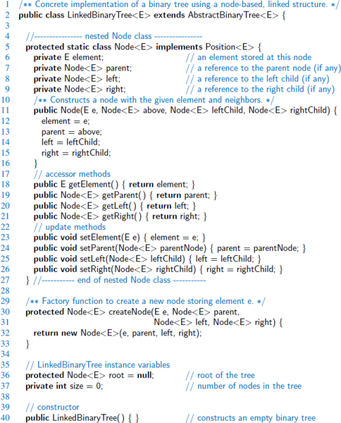
Code Fragment 8.8: An implementation of the LinkedBinaryTree class. (Continues in Code Fragments 8.9–8.11.)

Code Fragment 8.9: An implementation of the LinkedBinaryTree class. (Continued from Code Fragment 8.8; continues in Code Fragments 8.10 and 8.11.)

Code Fragment 8.10: An implementation of the LinkedBinaryTree class. (Continued from Code Fragments 8.8 and 8.9; continues in Code Fragment 8.11.)

Code Fragment 8.11: An implementation of the LinkedBinaryTree class. (Continued from Code Fragments 8.8–8.10.)
Performance of the Linked Binary Tree Implementation
To summarize the efficiencies of the linked structure representation, we analyze the running times of the LinkedBinaryTree methods, including derived methods that are inherited from the AbstractTree and AbstractBinaryTree classes:
- The size method, implemented in LinkedBinaryTree, uses an instance variable storing the number of nodes of a tree and therefore takes O(1) time. Method isEmpty, inherited from AbstractTree, relies on a single call to size and thus takes O(1) time.
- The accessor methods root, left, right, and parent are implemented directly in LinkedBinaryTree and take O(1) time each. The sibling, children, and numChildren methods are derived in AbstractBinaryTree using on a constant number of calls to these other accessors, so they run in O(1) time as well.
- The isInternal and isExternal methods, inherited from the AbstractTree class, rely on a call to numChildren, and thus run in O(1) time as well. The isRoot method, also implemented in AbstractTree, relies on a comparison to the result of the root method and runs in O(1) time.
- The update method, set, clearly runs in O(1) time. More significantly, all of the methods addRoot, addLeft, addRight, attach, and remove run in O(1) time, as each involves relinking only a constant number of parent-child relationships per operation.
- Methods depth and height were each analyzed in Section 8.1.3. The depth method at position p runs in O(dp + 1) time where dp is its depth; the height method on the root of the tree runs in O(n) time.
The overall space requirement of this data structure is O(n), for a tree with n nodes, as there is an instance of the Node class for every node, in addition to the top-level size and root fields. Table 8.1 summarizes the performance of the linked structure implementation of a binary tree.
| Method | Running Time |
| size, isEmpty | O(1) |
| root, parent, left, right, sibling, children, numChildren | O(1) |
| isInternal, isExternal, isRoot | O(1) |
| addRoot, addLeft, addRight, set, attach, remove | O(1) |
| depth(p) | O(dp+1) |
| height | O(n) |
Table 8.1: Running times for the methods of an n-node binary tree implemented with a linked structure. The space usage is O(n).
8.3.2 Array-Based Representation of a Binary Tree
An alternative representation of a binary tree T is based on a way of numbering the positions of T. For every position p of T, let f(p) be the integer defined as follows.
- If p is the root of T, then f(p) = 0.
- If p is the left child of position q, then f(p) = 2 f(q) + 1.
- If p is the right child of position q, then f (p) = 2f(q) + 2.
The numbering function f is known as a level numbering of the positions in a binary tree T, for it numbers the positions on each level of T in increasing order from left to right. (See Figure 8.10.) Note well that the level numbering is based on potential positions within a tree, not the actual shape of a specific tree, so they are not necessarily consecutive. For example, in Figure 8.10(b), there are no nodes with level numbering 13 or 14, because the node with level numbering 6 has no children.

Figure 8.10: Binary tree level numbering: (a) general scheme; (b) an example.
The level numbering function f suggests a representation of a binary tree T by means of an array-based structure A, with the element at position p of T stored at index f(p) of the array. We show an example of an array-based representation of a binary tree in Figure 8.11.
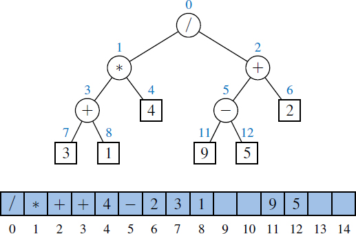
Figure 8.11: Representation of a binary tree by means of an array.
One advantage of an array-based representation of a binary tree is that a position p can be represented by the single integer f(p), and that position-based methods such as root, parent, left, and right can be implemented using simple arithmetic operations on the number f(p). Based on our formula for the level numbering, the left child of p has index 2 f(p) + 1, the right child of p has index 2 f(p) + 2, and the parent of p has index ![]() . We leave the details of a complete array-based implementation as Exercise R-8.16.
. We leave the details of a complete array-based implementation as Exercise R-8.16.
The space usage of an array-based representation depends greatly on the shape of the tree. Let n be the number of nodes of T, and let fM be the maximum value of f(p) over all the nodes of T. The array A requires length N = 1 + fM, since elements range from A[0] to A[fM]. Note that A may have a number of empty cells that do not refer to existing positions of T. In fact, in the worst case, N = 2n − 1, the justification of which is left as an exercise (R-8.14). In Section 9.3, we will see a class of binary trees, called “heaps” for which N = n. Thus, in spite of the worst-case space usage, there are applications for which the array representation of a binary tree is space efficient. Still, for general binary trees, the exponential worst-case space requirement of this representation is prohibitive.
Another drawback of an array representation is that many update operations for trees cannot be efficiently supported. For example, removing a node and promoting its child takes O(n) time because it is not just the child that moves locations within the array, but all descendants of that child.
8.3.3 Linked Structure for General Trees
When representing a binary tree with a linked structure, each node explicitly maintains fields left and right as references to individual children. For a general tree, there is no a priori limit on the number of children that a node may have. A natural way to realize a general tree T as a linked structure is to have each node store a single container of references to its children. For example, a children field of a node can be an array or list of references to the children of the node (if any). Such a linked representation is schematically illustrated in Figure 8.12.
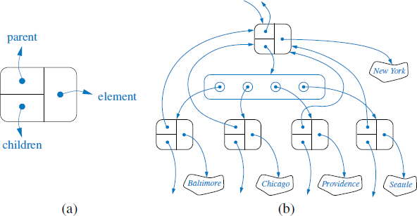
Figure 8.12: The linked structure for a general tree: (a) the structure of a node; (b) a larger portion of the data structure associated with a node and its children.
Table 8.2 summarizes the performance of the implementation of a general tree using a linked structure. The analysis is left as an exercise (R-8.13), but we note that, by using a collection to store the children of each position p, we can implement children(p) by simply iterating that collection.
| Method | Running Time |
| size, isEmpty | O(1) |
| root, parent, isRoot, isInternal, isExternal | O(1) |
| numChildren(p) | O(1) |
| children(p) | O(cp + 1) |
| depth(p) | O(dp + 1) |
| height | O(n) |
Table 8.2: Running times of the accessor methods of an n-node general tree implemented with a linked structure. We let cp denote the number of children of a position p, and dp its depth. The space usage is O(n).
8.4 Tree Traversal Algorithms
A traversal of a tree T is a systematic way of accessing, or “visiting,” all the positions of T. The specific action associated with the “visit” of a position p depends on the application of this traversal, and could involve anything from incrementing a counter to performing some complex computation for p. In this section, we describe several common traversal schemes for trees, implement them in the context of our various tree classes, and discuss several common applications of tree traversals.
8.4.1 Preorder and Postorder Traversals of General Trees
In a preorder traversal of a tree T, the root of T is visited first and then the subtrees rooted at its children are traversed recursively. If the tree is ordered, then the subtrees are traversed according to the order of the children. The pseudocode for the preorder traversal of the subtree rooted at a position p is shown in Code Fragment 8.12.

Code Fragment 8.12: Algorithm preorder for performing the preorder traversal of a subtree rooted at position p of a tree.
Figure 8.13 portrays the order in which positions of a sample tree are visited during an application of the preorder traversal algorithm.

Figure 8.13: Preorder traversal of an ordered tree, where the children of each position are ordered from left to right.
Postorder Traversal
Another important tree traversal algorithm is the postorder traversal. In some sense, this algorithm can be viewed as the opposite of the preorder traversal, because it recursively traverses the subtrees rooted at the children of the root first, and then visits the root (hence, the name “postorder”). Pseudocode for the postorder traversal is given in Code Fragment 8.13, and an example of a postorder traversal is portrayed in Figure 8.14.

Code Fragment 8.13: Algorithm postorder for performing the postorder traversal of a subtree rooted at position p of a tree.

Figure 8.14: Postorder traversal of the ordered tree of Figure 8.13.
Running-Time Analysis
Both preorder and postorder traversal algorithms are efficient ways to access all the positions of a tree. The analysis of either of these traversal algorithms is similar to that of algorithm height, given in Code Fragment 8.5 of Section 8.1.3. At each position p, the nonrecursive part of the traversal algorithm requires time O(cp + 1), where cp is the number of children of p, under the assumption that the “visit” itself takes O(1) time. By Proposition 8.4, the overall running time for the traversal of tree T is O(n), where n is the number of positions in the tree. This running time is asymptotically optimal since the traversal must visit all n positions of the tree.
8.4.2 Breadth-First Tree Traversal
Although the preorder and postorder traversals are common ways of visiting the positions of a tree, another approach is to traverse a tree so that we visit all the positions at depth d before we visit the positions at depth d + 1. Such an algorithm is known as a breadth-first traversal.
A breadth-first traversal is a common approach used in software for playing games. A game tree represents the possible choices of moves that might be made by a player (or computer) during a game, with the root of the tree being the initial configuration for the game. For example, Figure 8.15 displays a partial game tree for Tic-Tac-Toe.

Figure 8.15: Partial game tree for Tic-Tac-Toe when ignoring symmetries; annotations denote the order in which positions are visited in a breadth-first tree traversal.
A breadth-first traversal of such a game tree is often performed because a computer may be unable to explore a complete game tree in a limited amount of time. So the computer will consider all moves, then responses to those moves, going as deep as computational time allows.
Pseudocode for a breadth-first traversal is given in Code Fragment 8.14. The process is not recursive, since we are not traversing entire subtrees at once. We use a queue to produce a FIFO (i.e., first-in first-out) semantics for the order in which we visit nodes. The overall running time is O(n), due to the n calls to enqueue and n calls to dequeue.

Code Fragment 8.14: Algorithm for performing a breadth-first traversal of a tree.
8.4.3 Inorder Traversal of a Binary Tree
The standard preorder, postorder, and breadth-first traversals that were introduced for general trees can be directly applied to binary trees. In this section, we will introduce another common traversal algorithm specifically for a binary tree.
During an inorder traversal, we visit a position between the recursive traversals of its left and right subtrees. The inorder traversal of a binary tree T can be informally viewed as visiting the nodes of T “from left to right.” Indeed, for every position p, the inorder traversal visits p after all the positions in the left subtree of p and before all the positions in the right subtree of p. Pseudocode for the inorder traversal algorithm is given in Code Fragment 8.15, and an example of an inorder traversal is portrayed in Figure 8.16.

Code Fragment 8.15: Algorithm inorder for performing an inorder traversal of a subtree rooted at position p of a binary tree.
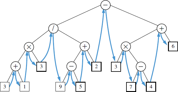
Figure 8.16: Inorder traversal of a binary tree.
The inorder traversal algorithm has several important applications. When using a binary tree to represent an arithmetic expression, as in Figure 8.16, the inorder traversal visits positions in a consistent order with the standard representation of the expression, as in 3 + 1 × 3/9 − 5 + 2... (albeit without parentheses).
Binary Search Trees
An important application of the inorder traversal algorithm arises when we store an ordered sequence of elements in a binary tree, defining a structure we call a binary search tree. Let S be a set whose unique elements have an order relation. For example, S could be a set of integers. A binary search tree for S is a proper binary tree T such that, for each internal position p of T:
- Position p stores an element of S, denoted as e(p).
- Elements stored in the left subtree of p (if any) are less than e(p).
- Elements stored in the right subtree of p (if any) are greater than e(p).
An example of a binary search tree is shown in Figure 8.17. The above properties assure that an inorder traversal of a binary search tree T visits the elements in nondecreasing order.
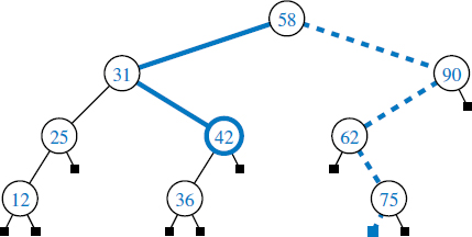
Figure 8.17: A binary search tree storing integers. The solid path is traversed when searching (successfully) for 42. The dashed path is traversed when searching (unsuccessfully) for 70.
We can use a binary search tree T for set S to find whether a given search value v is in S, by traversing a path down the tree T, starting at the root. At each internal position p encountered, we compare our search value v with the element e(p) stored at p. If v < e(p), then the search continues in the left subtree of p. If v = e(p), then the search terminates successfully. If v > e(p), then the search continues in the right subtree of p. Finally, if we reach a leaf, the search terminates unsuccessfully. In other words, a binary search tree can be viewed as a binary decision tree (recall Example 8.5), where the question asked at each internal node is whether the element at that node is less than, equal to, or larger than the element being searched for. We illustrate several examples of the search operation in Figure 8.17.
Note that the running time of searching in a binary search tree T is proportional to the height of T. Recall from Proposition 8.7 that the height of a binary tree with n nodes can be as small as log(n + 1) − 1 or as large as n − 1. Thus, binary search trees are most efficient when they have small height. Chapter 11 is devoted to the study of search trees.
8.4.4 Implementing Tree Traversals in Java
When first defining the tree ADT in Section 8.1.2, we stated that tree T must include the following supporting methods:
| iterator(): | Returns an iterator for all elements in the tree. |
| positions(): | Returns an iterable collection of all positions of the tree. |
At that time, we did not make any assumption about the order in which these iterations report their results. In this section, we will demonstrate how any of the tree traversal algorithms we have introduced can be used to produce these iterations as concrete implementations within the AbstractTree or AbstractBinaryTree base classes.
First, we note that an iteration of all elements of a tree can easily be produced if we have an iteration of all positions of that tree. Code Fragment 8.16 provides an implementation of the iterator() method by adapting an iteration produced by the positions() method. In fact, this is the identical approach we used in Code Fragment 7.14 of Section 7.4.2 for the LinkedPositionalList class.

Code Fragment 8.16: Iterating all elements of an AbstractTree instance, based upon an iteration of the positions of the tree.
To implement the positions() method, we have a choice of tree traversal algorithms. Given that there are advantages to each of those traversal orders, we provide public implementations of each strategy that can be called directly by a user of our class. We can then trivially adapt one of those as a default order for the positions method of the AbstractTree class. For example, on the following page we will define a public method, preorder(), that returns an iteration of the positions of a tree in preorder; Code Fragment 8.17 demonstrates how the positions() method can be trivially defined to rely on that order.
Code Fragment 8.17: Defining preorder as the default traversal algorithm for the public positions method of an abstract tree.
Preorder Traversals
We begin by considering the preorder traversal algorithm. Our goal is to provide a public method preorder(), as part of the AbstractTree class, which returns an iterable container of the positions of the tree in preorder. For ease of implementation, we choose to produce a snapshot iterator, as defined in Section 7.4.2, returning a list of all positions. (Exercise C-8.47 explores the goal of implementing a lazy iterator that reports positions in preorder.)
We begin by defining a private utility method, preorderSubtree, given in Code Fragment 8.18, which allows us to parameterize the recursive process with a specific position of the tree that serves as the root of a subtree to traverse. (We also pass a list as a parameter that serves as a buffer to which “visited” positions are added.)

Code Fragment 8.18: A recursive subroutine for performing a preorder traversal of the subtree rooted at position p of a tree. This code should be included within the body of the AbstractTree class.
The preorderSubtree method follows the high-level algorithm originally described as pseudocode in Code Fragment 8.12. It has an implicit base case, as the for loop body never executes if a position has no children.
The public preorder method, shown in Code Fragment 8.19, has the responsibility of creating an empty list for the snapshot buffer, and invoking the recursive method at the root of the tree (assuming the tree is nonempty). We rely on a java.util.ArrayList instance as an Iterable instance for the snapshot buffer.

Code Fragment 8.19: A public method that performs a preorder traversal of an entire tree. This code should be included within the body of the AbstractTree class.
Postorder Traversal
We implement a postorder traversal using a similar design as we used for a preorder traversal. The only difference is that a “visited” position is not added to a postorder snapshot until after all of its subtrees have been traversed. Both the recursive utility and the top-level public method are given in Code Fragment 8.20.

Code Fragment 8.20: Support for performing a postorder traversal of a tree. This code should be included within the body of the AbstractTree class.
Breadth-First Traversal
On the following page, we will provide an implementation of the breadth-first traversal algorithm in the context of our AbstractTree class (Code Fragment 8.21). Recall that the breadth-first traversal algorithm is not recursive; it relies on a queue of positions to manage the traversal process. We will use the LinkedQueue class from Section 6.2.3, although any implementation of the queue ADT would suffice.
Inorder Traversal for Binary Trees
The preorder, postorder, and breadth-first traversal algorithms are applicable to all trees. The inorder traversal algorithm, because it explicitly relies on the notion of a left and right child of a node, only applies to binary trees. We therefore include its definition within the body of the AbstractBinaryTree class. We use a similar design to our preorder and postorder traversals, with a private recursive utility for traversing subtrees. (See Code Fragment 8.22.)
For many applications of binary trees (for example, see Chapter 11), an inorder traversal is the most natural order. Therefore, Code Fragment 8.22 makes it the default for the AbstractBinaryTree class by overriding the positions method that was inherited from the AbstractTree class. Because the iterator() method relies on positions(), it will also use inorder when reporting the elements of a binary tree.

Code Fragment 8.21: An implementation of a breadth-first traversal of a tree. This code should be included within the body of the AbstractTree class.

Code Fragment 8.22: Support for performing an inorder traversal of a binary tree, and for making that order the default traversal for binary trees. This code should be included within the body of the AbstractBinaryTree class.
8.4.5 Applications of Tree Traversals
In this section, we demonstrate several representative applications of tree traversals, including some customizations of the standard traversal algorithms.
Table of Contents
When using a tree to represent the hierarchical structure of a document, a preorder traversal of the tree can be used to produce a table of contents for the document. For example, the table of contents associated with the tree from Figure 8.13 is displayed in Figure 8.18. Part (a) of that figure gives a simple presentation with one element per line; part (b) shows a more attractive presentation, produced by indenting each element based on its depth within the tree.

Figure 8.18: Table of contents for a document represented by the tree in Figure 8.13: (a) without indentation; (b) with indentation based on depth within the tree.
The unindented version of the table of contents can be produced with the following code, given a tree T supporting the preorder( ) method:
for (Position<E> p : T.preorder())
   System.out.println(p.getElement());
To produce the presentation of Figure 8.18(b), we indent each element with a number of spaces equal to twice the element's depth in the tree (hence, the root element was unindented). If we assume that method, spaces(n), produces a string of n spaces, we could replace the body of the above loop with the statement System.out.println(spaces(2*T.depth(p)) + p.getElement()). Unfortunately, although the work to produce the preorder traversal runs in O(n) time, based on the analysis of Section 8.4.1, the calls to depth incur a hidden cost. Making a call to depth from every position of the tree results in O(n2) worst-case time, as noted when analyzing the algorithm heightBad in Section 8.1.3.
A preferred approach to producing an indented table of contents is to redesign a top-down recursion that includes the current depth as an additional parameter. Such an implementation is provided in Code Fragment 8.23. This implementation runs in worst-case O(n) time (except, technically, the time it takes to print strings of increasing lengths).

Code Fragment 8.23: Efficient recursion for printing indented version of a pre-order traversal. To print an entire tree T, the recursion should be started with form printPreorderIndent(T, T.root(), 0).
In the example of Figure 8.18, we were fortunate in that the numbering was embedded within the elements of the tree. More generally, we might be interested in using a preorder traversal to display the structure of a tree, with indentation and also explicit numbering that was not present in the tree. For example, we might display the tree from Figure 8.2 beginning as:
Electronics R'Us
  1 R&D
  2 Sales
    2.1 Domestic
    2.2 International
      2.2.1 Canada
      2.2.2 S. America
This is more challenging, because the numbers used as labels are implicit in the structure of the tree. A label depends on the path from the root to the current position. To accomplish our goal, we add an additional parameter to the recursive signature. We send a list of integers representing the labels leading to a particular position. For example, when visiting the node Domestic above, we will send the list of values {2, 1} that comprise its label.
At the implementation level, we wish to avoid the inefficiency of duplicating such lists when sending a new parameter from one level of the recursion to the next. A standard solution is to pass the same list instance throughout the recursion. At one level of the recursion, a new entry is temporarily added to the end of the list before making further recursive calls. In order to “leave no trace,” the extraneous entry must later be removed from the list by the same recursive call that added it. An implementation based on this approach is given in Code Fragment 8.24.

Code Fragment 8.24: Efficient recursion for printing an indented and labeled presentation of a preorder traversal.
Computing Disk Space
In Example 8.1, we considered the use of a tree as a model for a file-system structure, with internal positions representing directories and leaves representing files. In fact, when introducing the use of recursion back in Chapter 5, we specifically examined the topic of file systems (see Section 5.1.4). Although we did not explicitly model it as a tree at that time, we gave an implementation of an algorithm for computing the disk usage (Code Fragment 5.5).
The recursive computation of disk space is emblematic of a postorder traversal, as we cannot effectively compute the total space used by a directory until after we know the space that is used by its children directories. Unfortunately, the formal implementation of postorder, as given in Code Fragment 8.20, does not suffice for this purpose. We would like to have a mechanism for children to return information to the parent as part of the traversal process. A custom solution to the disk space problem, with each level of recursion providing a return value to the (parent) caller, is provided in Code Fragment 8.25.

Code Fragment 8.25: Recursive computation of disk space for a tree. We assume that each tree element reports the local space used at that position.
Parenthetic Representations of a Tree
It is not possible to reconstruct a general tree, given only the preorder sequence of elements, as in Figure 8.18a. Some additional context is necessary for the structure of the tree to be well defined. The use of indentation or numbered labels provides such context, with a very human-friendly presentation. However, there are more concise string representations of trees that are computer-friendly.
In this section, we explore one such representation. The parenthetic string representation P(T) of tree T is recursively defined. If T consists of a single position p, then P(T) = p.getElement(). Otherwise, it is defined recursively as,
P(T) = p.getElement() + "(" + P(T1) + ", " + ... + ", " + P(Tk) + ")"
where p is the root of T and T1, T2, ..., Tk are the subtrees rooted at the children of p, which are given in order if T is an ordered tree. We are using “+” here to denote string concatenation. As an example, the parenthetic representation of the tree of Figure 8.2 would appear as follows (line breaks are cosmetic):
Electronics R'Us (R&D, Sales (Domestic, International (Canada,
S. America, Overseas (Africa, Europe, Asia, Australia))),
Purchasing, Manufacturing (TV, CD, Tuner))
Although the parenthetic representation is essentially a preorder traversal, we cannot easily produce the additional punctuation using the formal implementation of preorder. The opening parenthesis must be produced just before the loop over a position's children, the separating commas between children, and the closing parenthesis just after the loop completes. The Java method parenthesize, shown in Code Fragment 8.26, is a custom traversal that prints such a parenthetic string representation of a tree T.
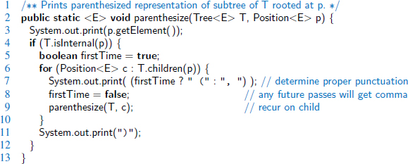
Code Fragment 8.26: Method that prints parenthetic string representation of a tree.
Using Inorder Traversal for Tree Drawing
An inorder traversal can be applied to the problem of computing a graphical layout of a binary tree, as shown in Figure 8.19. We assume the convention, common to computer graphics, that x-coordinates increase left to right and y-coordinates increase top to bottom, so that the origin is in the upper left corner of the drawing.

Figure 8.19: An inorder drawing of a binary tree.
The geometry is determined by an algorithm that assigns x- and y-coordinates to each position p of a binary tree T using the following two rules:
- x(p) is the number of positions visited before p in an inorder traversal of T.
- y(p) is the depth of p in T.
Code Fragment 8.27 provides an implementation of a recursive method that assigns x- and y-coordinates to positions of a tree in this manner. Depth information is passed from one level of the recursion to another, as done in our earlier example for indentation. To maintain an accurate value for the x-coordinate as the traversal proceeds, the method must be provided with the value of x that should be assigned to the leftmost node of the current subtree, and it must return to its parent a revised value of x that is appropriate for the first node drawn to the right of the subtree.

Code Fragment 8.27: Recursive method for computing coordinates at which to draw positions of a binary tree. We assume that the element type for the tree supports setX and setY methods. The initial call should be layout(T, T.root(), 0, 0).
8.4.6 Euler Tours
The various applications described in Section 8.4.5 demonstrate the great power of recursive tree traversals, but they also show that not every application strictly fits the mold of a preorder, postorder, or inorder traversal. We can unify the tree-traversal algorithms into a single framework known as an Euler tour traversal. The Euler tour traversal of a tree T can be informally defined as a “walk” around T, where we start by going from the root toward its leftmost child, viewing the edges of T as being “walls” that we always keep to our left. (See Figure 8.20.)

Figure 8.20: Euler tour traversal of a tree.
The complexity of the walk is O(n), for a tree with n nodes, because it progresses exactly two times along each of the n − 1 edges of the tree—once going downward along the edge, and later going upward along the edge. To unify the concept of preorder and postorder traversals, we can view there being two notable “visits” to each position p:
- A “pre visit” occurs when first reaching the position, that is, when the walk passes immediately left of the node in our visualization.
- A “post visit” occurs when the walk later proceeds upward from that position, that is, when the walk passes to the right of the node in our visualization.
The process of an Euler tour can be naturally viewed as recursive. In between the “pre visit” and “post visit” of a given position will be a recursive tour of each of its subtrees. Looking at Figure 8.20 as an example, there is a contiguous portion of the entire tour that is itself an Euler tour of the subtree of the node with element “/”. That tour contains two contiguous subtours, one traversing that position's left subtree and another traversing the right subtree.
In the special case of a binary tree, we can designate the time when the walk passes immediately below a node as an “in visit” event. This will be just after the tour of its left subtree (if any), but before the tour of its right subtree (if any).
The pseudocode for an Euler tour traversal of a subtree rooted at a position p is shown in Code Fragment 8.28.

Code Fragment 8.28: Algorithm eulerTour for performing an Euler tour traversal of a subtree rooted at position p of a tree.
The Euler tour traversal extends the preorder and postorder traversals, but it can also perform other kinds of traversals. For example, suppose we wish to compute the number of descendants of each position p in an n-node binary tree. We start an Euler tour by initializing a counter to 0, and then increment the counter during the “pre visit” for each position. To determine the number of descendants of a position p, we compute the difference between the values of the counter from when the pre-visit occurs and when the post-visit occurs, and add 1 (for p). This simple rule gives us the number of descendants of p, because each node in the subtree rooted at p is counted between p's visit on the left and p's visit on the right. Therefore, we have an O(n)-time method for computing the number of descendants of each node.
For the case of a binary tree, we can customize the algorithm to include an explicit “in visit” action, as shown in Code Fragment 8.29.

Code Fragment 8.29: Algorithm eulerTourBinary for performing an Euler tour traversal of a subtree rooted at position p of a binary tree.
For example, a binary Euler tour can produce a traditional parenthesized arithmetic expression, such as "((((3+1)x3)/((9−5)+2))−((3x(7−4))+6))" for the tree in Figure 8.20, as follows:
- “Pre visit” action: if the position is internal, print “(”.
- “In visit” action: print the value or operator stored at the position.
- “Post visit” action: if the position is internal, print “)”.
8.5 Exercises
Reinforcement
| R-8.1 | The following questions refer to the tree of Figure 8.3.
|
| R-8.2 | Show a tree achieving the worst-case running time for algorithm depth. |
| R-8.3 | Give a justification of Proposition 8.3. |
| R-8.4 | What is the running time of a call to T.height(p) when called on a position p distinct from the root of tree T? (See Code Fragment 8.5.) |
| R-8.5 | Describe an algorithm, relying only on the BinaryTree operations, that counts the number of leaves in a binary tree that are the left child of their respective parent. |
| R-8.6 | Let T be an n-node binary tree that may be improper. Describe how to represent T by means of a proper binary tree T′ with O(n) nodes. |
| R-8.7 | What are the minimum and maximum number of internal and external nodes in an improper binary tree with n nodes? |
| R-8.8 | Answer the following questions so as to justify Proposition 8.7.
|
| R-8.9 | Give a proof by induction of Proposition 8.8. |
| R-8.10 | Find the value of the arithmetic expression associated with each subtree of the binary tree of Figure 8.6. |
| R-8.11 | Draw an arithmetic expression tree that has four external nodes, storing the numbers 1, 5, 6, and 7 (with each number stored in a distinct external node, but not necessarily in this order), and has three internal nodes, each storing an operator from the set {+, −, *, / }, so that the value of the root is 21. The operators may return and act on fractions, and an operator may be used more than once. |
| R-8.12 | Draw the binary tree representation of the following arithmetic expression: “(((5 + 2) * (2 − 1))/((2 + 9) + ((7 − 2) − 1)) * 8)”. |
| R-8.13 | Justify Table 8.2, summarizing the running time of the methods of a tree represented with a linked structure, by providing, for each method, a description of its implementation, and an analysis of its running time. |
| R-8.14 | Let T be a binary tree with n nodes, and let f() be the level numbering function of the positions of T, as given in Section 8.3.2.
|
| R-8.15 | Show how to use an Euler tour traversal to compute the level number f(p), as defined in Section 8.3.2, of each position in a binary tree T. |
| R-8.16 | Let T be a binary tree with n positions that is realized with an array representation A, and let f () be the level numbering function of the positions of T, as given in Section 8.3.2. Give pseudocode descriptions of each of the methods root, parent, left, right, isExternal, and isRoot. |
| R-8.17 | Our definition of the level numbering function f(p), as given in Section 8.3.2, begins with the root having number 0. Some people prefer to use a level numbering g(p) in which the root is assigned number 1, because it simplifies the arithmetic for finding neighboring positions. Redo Exercise R-8.16, but assuming that we use a level numbering g(p) in which the root is assigned number 1. |
| R-8.18 | In what order are positions visited during a preorder traversal of the tree of Figure 8.6? |
| R-8.19 | In what order are positions visited during a postorder traversal of the tree of Figure 8.6? |
| R-8.20 | Let T be an ordered tree with more than one node. Is it possible that the preorder traversal of T visits the nodes in the same order as the postorder traversal of T ? If so, give an example; otherwise, explain why this cannot occur. Likewise, is it possible that the preorder traversal of T visits the nodes in the reverse order of the postorder traversal of T? If so, give an example; otherwise, explain why this cannot occur. |
| R-8.21 | Answer the previous question for the case when T is a proper binary tree with more than one node. |
| R-8.22 | Draw a binary tree T that simultaneously satisfies the following:
|
| R-8.23 | Consider the example of a breadth-first traversal given in Figure 8.15. Using the annotated numbers from that figure, describe the contents of the queue before each pass of the while loop in Code Fragment 8.14. To get started, the queue has contents {1} before the first pass, and contents {2,3,4} before the second pass. |
| R-8.24 | Give the output of the method parenthesize(T, T.root()), as described in Code Fragment 8.26, when T is the tree of Figure 8.6. |
| R-8.25 | Describe a modification to parenthesize, from Code Fragment 8.26, that relies on the length() method for the String class to output the parenthetic representation of a tree with line breaks added to display the tree in a text window that is 80 characters wide. |
| R-8.26 | What is the running time of parenthesize(T, T.root()), as given in Code Fragment 8.26, for a tree T with n nodes? |
Creativity
| C-8.27 | Describe an efficient algorithm for converting a fully balanced string of parentheses into an equivalent tree. The tree associated with such a string is defined recursively. The outermost pair of balanced parentheses is associated with the root and each substring inside this pair, defined by the substring between two balanced parentheses, is associated with a subtree of this root. |
| C-8.28 | The path length of a tree T is the sum of the depths of all positions in T. Describe a linear-time method for computing the path length of a tree T. |
| C-8.29 | Define the internal path length, I(T), of a tree T to be the sum of the depths of all the internal positions in T. Likewise, define the external path length, E(T), of a tree T to be the sum of the depths of all the external positions in T. Show that if T is a proper binary tree with n positions, then E(T) = I(T) + n − 1. |
| C-8.30 | Let T be a (not necessarily proper) binary tree with n nodes, and let D be the sum of the depths of all the external nodes of T. Show that if T has the minimum number of external nodes possible, then D is O(n) and if T has the maximum number of external nodes possible, then D is O(nlog n). |
| C-8.31 | Let T be a (possibly improper) binary tree with n nodes, and let D be the sum of the depths of all the external nodes of T. Describe a configuration for T such that D is Ω(n2). Such a tree would be the worst case for the asymptotic running time of method heightBad (Code Fragment 8.4). |
| C-8.32 | For a tree T, let nI denote the number of its internal nodes, and let nE denote the number of its external nodes. Show that if every internal node in T has exactly 3 children, then nE = 2nI + 1. |
| C-8.33 | Two ordered trees T′ and T″ are said to be isomorphic if one of the following holds:
Design an algorithm that tests whether two given ordered trees are isomorphic. What is the running time of your algorithm? |
| C-8.34 | Show that there are more than 2n improper binary trees with n internal nodes such that no pair are isomorphic (see Exercise C-8.33). |
| C-8.35 | If we exclude isomorphic trees (see Exercise C-8.33), exactly how many proper binary trees exist with exactly 4 leaves? |
| C-8.36 | Add support in LinkedBinaryTree for a method, pruneSubtree(p), that removes the entire subtree rooted at position p, making sure to maintain an accurate count of the size of the tree. What is the running time of your implementation? |
| C-8.37 | Add support in LinkedBinaryTree for a method, swap(p, q), that has the effect of restructuring the tree so that the node referenced by p takes the place of the node referenced by q, and vice versa. Make sure to properly handle the case when the nodes are adjacent. |
| C-8.38 | We can simplify parts of our LinkedBinaryTree implementation if we make use of of a single sentinel node, such that the sentinel is the parent of the real root of the tree, and the root is referenced as the left child of the sentinel. Furthermore, the sentinel will take the place of null as the value of the left or right member for a node without such a child. Give a new implementation of the update methods remove and attach, assuming such a representation. |
| C-8.39 | Describe how to clone a LinkedBinaryTree instance representing a proper binary tree, with use of the attach method. |
| C-8.40 | Describe how to clone a LinkedBinaryTree instance representing a (not necessarily proper) binary tree, with use of the addLeft and addRight methods. |
| C-8.41 | Modify the LinkedBinaryTree class to formally support the Cloneable interface, as described in Section 3.6. |
| C-8.42 | Give an efficient algorithm that computes and prints, for every position p of a tree T, the element of p followed by the height of p's subtree. |
| C-8.43 | Give an O(n)-time algorithm for computing the depths of all positions of a tree T, where n is the number of nodes of T. |
| C-8.44 | The balance factor of an internal position p of a proper binary tree is the difference between the heights of the right and left subtrees of p. Show how to specialize the Euler tour traversal of Section 8.4.6 to print the balance factors of all the internal nodes of a proper binary tree. |
| C-8.45 | Design algorithms for the following operations for a binary tree T:
What are the worst-case running times of your algorithms? |
| C-8.46 | Describe, in pseudocode, a nonrecursive method for performing an inorder traversal of a binary tree in linear time. |
| C-8.47 | To implement the preorder method of the AbstractTree class, we relied on the convenience of creating a snapshot. Reimplement a preorder method that creates a lazy iterator. (See Section 7.4.2 for discussion of iterators.) |
| C-8.48 | Repeat Exercise C-8.47, implementing the postorder method of the AbstractTree class. |
| C-8.49 | Repeat Exercise C-8.47, implementing the AbstractBinaryTree's inorder method. |
| C-8.50 | Algorithm preorderDraw draws a binary tree T by assigning x- and y-coordinates to each position p such that x(p) is the number of nodes preceding p in the preorder traversal of T and y(p) is the depth of p in T.
|
| C-8.51 | Redo the previous problem for the algorithm postorderDraw that is similar to preorderDraw except that it assigns x(p) to be the number of nodes preceding position p in the postorder traversal. |
| C-8.52 | We can define a binary tree representation T′ for an ordered general tree T as follows (see Figure 8.21):
Given such a representation T′ of a general ordered tree T, answer each of the following questions:
Figure 8.21: Representation of a tree with a binary tree: (a) tree T; (b) binary tree T′ for T. The dashed edges connect nodes of T′ that are siblings in T. |
| C-8.53 | Design an algorithm for drawing general trees, using a style similar to the inorder traversal approach for drawing binary trees. |
| C-8.54 | Let the rank of a position p during a traversal be defined such that the first element visited has rank 1, the second element visited has rank 2, and so on. For each position p in a tree T, let pre(p) be the rank of p in a preorder traversal of T, let post(p) be the rank of p in a postorder traversal of T, let depth(p) be the depth of p, and let desc(p) be the number of descendants of p, including p itself. Derive a formula defining post(p) in terms of desc(p), depth (p), and pre(p), for each node p in T. |
| C-8.55 | Let T be a tree with n positions. Define the lowest common ancestor (LCA) between two positions p and q as the lowest position in T that has both p and q as descendants (where we allow a position to be a descendant of itself). Given two positions p and q, describe an efficient algorithm for finding the LCA of p and q. What is the running time of your algorithm? |
| C-8.56 | Suppose each position p of a binary tree T is labeled with its value f(p) in a level numbering of T. Design a fast method for determining f(a) for the lowest common ancestor (LCA), a, of two positions p and q in T, given f(p) and f(q). You do not need to find position a, just value f(a). |
| C-8.57 | Let T be a binary tree with n positions, and, for any position p in T, let dp denote the depth of p in T. The distance between two positions p and q in T is dp + dq − 2da, where a is the lowest common ancestor (LCA) of p and q. The diameter of T is the maximum distance between two positions in T. Describe an efficient algorithm for finding the diameter of T. What is the running time of your algorithm? |
| C-8.58 | The indented parenthetic representation of a tree T is a variation of the parenthetic representation of T (see Code Fragment 8.26) that uses indentation and line breaks as illustrated in Figure 8.22. Give an algorithm that prints this representation of a tree.
Figure 8.22: (a) Tree T; (b) indented parenthetic representation of T. |
| C-8.59 | As mentioned in Exercise C-6.19, postfix notation is an unambiguous way of writing an arithmetic expression without parentheses. It is defined so that if “(exp1) op (exp2)” is a normal (infix) fully parenthesized expression with operation op, then its postfix equivalent is “pexp1 pexp2 op”, where pexp1 is the postfix version of exp1 and pexp2 is the postfix version of exp2. The postfix version of a single number or variable is just that number or variable. So, for example, the postfix version of the infix expression “((5 + 2) * (8 − 3))/4” is “5 2 + 8 3 − * 4 /”. Give an efficient algorithm for converting an infix arithmetic expression to its equivalent postfix notation. (Hint: First convert the infix expression into its equivalent binary tree representation.) |
| C-8.60 | Let T be a binary tree with n positions. Define a Roman position to be a position p in T, such that the number of descendants in p's left subtree differ from the number of descendants in p's right subtree by at most 5. Describe a linear-time method for finding each position p of T, such that p is not a Roman position, but all of p's descendants are Roman. |

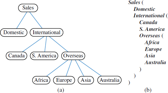
Projects
| P-8.61 | Implement the binary tree ADT using the array-based representation described in Section 8.3.2. |
| P-8.62 | Implement the tree ADT using a linked structure as described in Section 8.3.3. Provide a reasonable set of update methods for your tree. |
| P-8.63 | Implement the tree ADT using the binary tree representation described in Exercise C-8.52. You may adapt the LinkedBinaryTree implementation. |
| P-8.64 | The memory usage for the LinkedBinaryTree class can be streamlined by removing the parent reference from each node, and instead implementing a Position as an object that keeps a list of nodes representing the entire path from the root to that position. Reimplement the LinkedBinaryTree class using this strategy. |
| P-8.65 | Write a program that takes as input a fully parenthesized, arithmetic expression and converts it to a binary expression tree. Your program should display the tree in some way and also print the value associated with the root. For an additional challenge, allow the leaves to store variables of the form x1, x2, x3, and so on, which are initially 0 and which can be updated interactively by your program, with the corresponding update in the printed value of the root of the expression tree. |
| P-8.66 | A slicing floor plan divides a rectangle with horizontal and vertical sides using horizontal and vertical cuts. (See Figure 8.23a.) A slicing floor plan can be represented by a proper binary tree, called a slicing tree, whose internal nodes represent the cuts, and whose external nodes represent the basic rectangles into which the floor plan is decomposed by the cuts. (See Figure 8.23b.) The compaction problem for a slicing floor plan is defined as follows. Assume that each basic rectangle of a slicing floor plan is assigned a minimum width w and a minimum height h. The compaction problem is to find the smallest possible height and width for each rectangle of the slicing floor plan that is compatible with the minimum dimensions of the basic rectangles. Namely, this problem requires the assignment of values h(p) and w(p) to each position p of the slicing tree such that:
Figure 8.23: (a) Slicing floor plan; (b) slicing tree associated with the floor plan.
Design a data structure for slicing floor plans that supports the operations:
|
| P-8.67 | Write a program that can play Tic-Tac-Toe effectively. (See Section 3.1.5.) Todo this, you will need to create a game tree T, which is a tree where each position corresponds to a game configuration, which, in this case, is a representation of the Tic-Tac-Toe board. (See Section 8.4.2.) The root corresponds to the initial configuration. For each internal position p in T, the children of p correspond to the game states we can reach from p's game state in a single legal move for the appropriate player, A (the first player) or B (the second player). Positions at even depths correspond to moves for A and positions at odd depths correspond to moves for B. Leaves are either final game states or are at a depth beyond which we do not want to explore. We score each leaf with a value that indicates how good this state is for player A. In large games, like chess, we have to use a heuristic scoring function, but for small games, like Tic-Tac-Toe, we can construct the entire game tree and score leaves as +1, 0, −1, indicating whether player A has a win, draw, or lose in that configuration. A good algorithm for choosing moves is minimax. In this algorithm, we assign a score to each internal position p in T, such that if p represents A's turn, we compute p's score as the maximum of the scores of p's children (which corresponds to A's optimal play from p). If an internal node p represents B's turn, then we compute p's score as the minimum of the scores of p's children (which corresponds to B's optimal play from p). |
| P-8.68 | Write a program that takes as input a general tree T and a position p of T and converts T to another tree with the same set of position adjacencies, but now with p as its root. |
| P-8.69 | Write a program that draws a binary tree. |
| P-8.70 | Write a program that draws a general tree. |
| P-8.71 | Write a program that can input and display a person's family tree. |
| P-8.72 | Write a program that visualizes an Euler tour traversal of a proper binary tree, including the movements from node to node and the actions associated with visits on the left, from below, and on the right. Illustrate your program by having it compute and display preorder labels, inorder labels, postorder labels, ancestor counts, and descendant counts for each node in the tree (not necessarily all at the same time). |


Chapter Notes
Discussions of the classic preorder, inorder, and postorder tree traversal methods can be found in Knuth's Fundamental Algorithms book [60]. The Euler tour traversal technique comes from the parallel algorithms community; it is introduced by Tarjan and Vishkin [86] and is discussed by JáJá [50] and by Karp and Ramachandran [55]. The algorithm for drawing a tree is generally considered to be a part of the “folklore” of graph-drawing algorithms. The reader interested in graph drawing is referred to the book by Di Battista, Eades, Tamassia, and Tollis [29] and the survey by Tamassia and Liotta [85]. The puzzle in Exercise R-8.11 was communicated by Micha Sharir.