
Chapter Seven. Database Design Theory
The goal of data independence has the direct implication that logical and physical database design are different disciplines: logical design is concerned with what the database looks like to the user, and physical design is concerned with how the logical design maps to physical storage. The primary focus of this chapter is on logical design, and I’ll use the unqualified term design to mean logical design specifically, until further notice.
One point I want to stress right away is this. Recall that “the” relvar constraint for relvar R can be regarded as the system’s approximation to the predicate for R; recall too that the predicate for R is the intended interpretation, or meaning, for R. It follows that constraints and predicates are highly relevant to the business of logical design! Indeed, logical design is, in essence, precisely a process of pinning down the predicates as carefully as possible and then mapping those predicates to relvars and constraints. Of course, those predicates are necessarily somewhat informal (they’re what some people like to call “business rules”); by contrast, the relvar and constraint definitions are necessarily formal.
Incidentally, the foregoing state of affairs explains why I’m not much of a fan of entity/relationship (E/R) modeling and similar pictorial methodologies. The problem with E/R diagrams and similar pictures is that they’re completely incapable of representing all but a few rather specialized constraints. Thus, although it might be OK to use such diagrams to explicate the overall design at a high level of abstraction, it’s misleading, and in some respects quite dangerous, to think of such a diagram as actually being the design in its entirety. Au contraire: the design is the relvars, which the diagrams do show, together with the constraints, which they don’t.
There’s another general point I need to make up front. Recall from Chapter 4 that views are supposed to look and feel just like base relvars (I don’t mean views defined as mere shorthands, I mean views that insulate the user from the “real” database in some way). In general, in fact, any given user interacts not with a database that contains only base relvars (the “real” database), but rather with what might be called a user database that contains some mixture of base relvars and views. Of course, that user database is supposed to look and feel like the real database to that user . . . and so it follows that all of the design principles to be discussed in this chapter apply equally well to such user databases, not just to the real database.
I feel compelled to make one further introductory remark. Several reviewers of earlier drafts of this chapter seemed to assume that what I was trying to do was teach elementary database design. But I wasn’t. You’re a database professional, so you’re supposed to be familiar with design basics already. So the purpose of the chapter is not to explain the design process as it’s actually carried out in practice; rather, the purpose is to reinforce certain aspects of design that you already know, by looking at them from a possibly unfamiliar perspective, and to explore certain other aspects that you might not already know. I don’t plan to spend a lot of time covering what should be familiar territory. Thus, for example, I deliberately won’t go into a lot of detail on second and third normal forms, because they’re part of conventional design wisdom and shouldn’t need any elaboration in a book of this nature (in any case, they’re not all that important in themselves except as a stepping-stone to Boyce/Codd normal form, which I will discuss in this chapter).
The Place of Design Theory
Design theory as such isn’t part of the relational model; rather, it’s a separate theory in its own right that builds on top of that model. (It’s appropriate to think of it as part of relational theory overall, but it’s not, to repeat, part of the model as such.) However, it does rely on certain fundamental notions—for example, the operators projection and join—that are part of the model.
And another thing: the design theory I’m talking about doesn’t really tell you how to do design! Rather, it tells you what goes wrong if you don’t design the database in the “obvious” way. Consider suppliers and parts, for example. The obvious design is the one I’ve been assuming in this book all along; I mean, it’s “obvious” that three relvars are necessary, that attribute STATUS belongs in relvar S, that attribute COLOR belongs in relvar P, that attribute QTY belongs in relvar SP, and so on. But why exactly are these things obvious? Well, suppose we tried a different design; for example, suppose we moved the STATUS attribute out of relvar S and into relvar SP (intuitively the wrong place for it, since status has to do with suppliers, not shipments). Figure 7-1 shows a sample value for this revised shipments relvar (which I’ll call STP to avoid confusion).
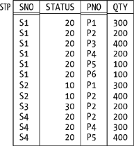
A glance at the figure is sufficient to show what’s wrong with this design: it’s redundant, in the sense that every tuple for supplier S1 tells us S1 has status 20, every tuple for supplier S2 tells us S2 has status 10, and so on. And design theory tells us that not designing the database in the obvious way will lead to such redundancy, and it also tells us the consequences of such redundancy. In other words, design theory is basically all about reducing redundancy, as we’ll soon see. For such reasons, design theory has been characterized—perhaps a little unkindly—as a good source of bad examples. What’s more, it has also been criticized on the grounds that it’s all just common sense anyway. I’ll come back to this criticism in the next section.
To put a more positive spin on matters, design theory can be useful in checking that designs produced via some other methodology don’t violate any formal design principles. Then again . . . the sad fact is, while those formal design principles do constitute the scientific part of the design discipline, there are numerous aspects of design that they simply don’t address at all. Database design is still largely subjective in nature; the formal principles I’m going to describe in this chapter represent the one small piece of science in what’s otherwise a mostly artistic endeavor.
So I want to consider the scientific part of design. To be specific, I want to examine two broad topics, normalization and orthogonality. Now, I assume you already know a lot about the first of these, at least. In particular, I assume you know that:
There are several different normal forms (first, second, third, and so on).
Loosely speaking, if relvar R is in (n+1)st normal form, then it’s certainly in n th normal form.
It’s possible for a relvar to be in n th normal form and not in (n+1)st normal form.
The higher the normal form the better, from a design point of view.
These ideas all rely on certain dependencies (in this context, just another term for integrity constraints).
I’d like to elaborate briefly on the last of these points. I’ve said that constraints in general are highly relevant to the design process. It turns out, however, that the particular constraints we’re talking about here—the so-called dependencies—enjoy certain formal properties that constraints in general don’t (so far as we know). I can’t get into this issue very deeply here; however, the basic point is that it’s possible to define certain inference rules for such dependencies, and it’s the existence of those inference rules that make it possible to develop the design theory that I’m going to describe.
To repeat, I assume you already know something about these matters. As noted in the previous section, however, I want to focus on aspects of the subject that you might not be so familiar with; I want to highlight the more important parts and downplay the others, and more generally I want to look at the whole subject from a perspective that might be a little different from what you’re used to.
Functional Dependencies and Boyce/Codd Normal Form
It’s well known that the notions of second normal form (2NF), third normal form (3NF), and Boyce/Codd normal form (BCNF) all depend on the notion of functional dependency . Here’s a precise definition:
Definition: Let A and B be subsets of the heading of relvar R. Then relvar R satisfies the functional dependency (FD) A → B if and only if, in every relation that’s a legal value for R, whenever two tuples have the same value for A, they also have the same value for B.
The FD A → B is read as "B is functionally dependent on A,” or "A functionally determines B,” or, more simply, just "A arrow B.”
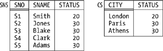
By way of example, suppose there’s an integrity constraint to the effect that if two suppliers are in the same city, then they must have the same status (see Figure 7-2, where I’ve changed the status for supplier S2 from 10 to 30 in order to conform to this hypothetical new constraint). Then the FD:
{ CITY } → { STATUS }
is satisfied by this revised form—let’s call it RS—of the suppliers relvar S. Note the braces, by the way; I use braces to stress the point that both sides of the FD are sets of attributes, even when (as in the example) the sets in question involve just a single attribute.

As the example indicates, the fact that some relvar R satisfies a given FD constitutes a database constraint in the sense of the previous chapter; more precisely, it constitutes a (single-relvar) constraint on that relvar R. For instance, the FD in the example is equivalent to the following Tutorial D constraint:
  CONSTRAINT RSC COUNT ( RS { CITY } ) =
                 COUNT ( RS { CITY, STATUS } ) ;
By the way, here’s a useful thing to remember: if relvar R satisfies the FD A → B, it necessarily satisfies the FD A’ → B’ for all supersets A’ of A and all subsets B’ of B. In other words, you can always add attributes to the left side or subtract them from the right side, and what you get will still be a valid FD.
At this point I need to introduce a couple of terms. The first is superkey . Basically, a superkey is a superset of a key (not necessarily a proper superset, of course); equivalently (with reference to the formal definition of key from Chapter 4), a subset SK of the heading of relvar R is a superkey for R if and only if it possesses the uniqueness property but not necessarily the irreducibility property. Thus, every key is a superkey, but most superkeys aren’t keys; for example, {SNO,CITY} is a superkey for relvar S but not a key. Observe in particular that the heading of relvar R is always a superkey for R.
Note
Important: If SK is a superkey for R and A is any subset of the heading of R, R necessarily satisfies the FD SK → A— because if two tuples of R have the same value for SK, then by definition they’re the very same tuple, and so they obviously have the same value for A. (I did touch on this point in Chapter 4, but there I talked in terms of keys, not superkeys.)
The other new term is trivial FD. Basically, an FD is trivial if there’s no way it can possibly be violated. For example, the following FDs are all trivially satisfied by any relvar that includes attributes called SNO, STATUS, and CITY:
  { CITY, STATUS } → { CITY }
  { SNO, CITY }    → { CITY }
  { CITY }         → { CITY }
  { SNO }          → { SNO }
In the first case, for instance, if two tuples have the same value for CITY and STATUS, they certainly have the same value for CITY. In fact, an FD is trivial if and only if the left side is a superset of the right side (again, not necessarily a proper superset). Of course, we don’t usually think about trivial FDs when we’re doing database design, because they’re, well, trivial; but when we’re trying to be formal and precise about these matters, we need to take all FDs into account, trivial ones as well as nontrivial.
Having pinned down the notion of FD precisely, I can now say that Boyce/Codd normal form (BCNF) is the normal form with respect to FDs—and, of course, I can also define it precisely:
Definition: Relvar R is in BCNF if and only if, for every nontrivial FD A → B satisfied by R, A is a superkey for R.
In other words, in a BCNF relvar, the only FDs are either trivial ones (we can’t get rid of those, obviously) or “arrows out of superkeys” (we can’t get rid of those, either). Or as some people like to say: Every fact is a fact about the key, the whole key, and nothing but the key— though I must immediately add that this informal characterization, intuitively pleasing though it is, isn’t really accurate, because it assumes among other things that there’s just one key.
I need to elaborate slightly on the previous paragraph. When I talk about “getting rid of” some FD, I fear I’m being a little sloppy once again. For example, the revised suppliers relvar RS of Figure 7-2 satisfies the FD {SNO} → {STATUS}; but if we decompose it—as we’re going to do in a moment—into relvars SNC and CS (where SNC has attributes SNO, SNAME, and CITY, and CS has attributes CITY and STATUS), that FD “disappears,” in a sense, and thus we have indeed “gotten rid of it.” But what does it mean to say the FD has disappeared? What’s happened is that it’s become a multi-relvar constraint (that is, a constraint that involves two or more relvars).[*] So the constraint certainly still exists—it just isn’t an FD any more. Similar remarks apply to all of my uses of the phrase “get rid of” in this chapter.
Finally, as I assume you know, the normalization discipline says that if relvar R is not in BCNF, it should be decomposed into smaller ones that are (where “smaller” means, basically, having fewer attributes). For example:
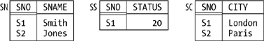
Relvar STP (see Figure 7-1) satisfies the FD {SNO} → {STATUS}, which is neither trivial nor “an arrow out of a superkey”—{SNO} isn’t a superkey for STP—and the relvar is thus not in BCNF (and of course it suffers from redundancy, as we saw earlier). So we decompose it into relvars SP and SS, say, where SP has attributes SNO, PNO, and QTY (as usual) and SS has attributes SNO and STATUS. (As an exercise, show sample values for relvars SP and SS corresponding to the STP value in Figure 7-1; convince yourself that SP and SS are in BCNF and that the decomposition eliminates the redundancy.)
Similarly, relvar RS (see Figure 7-2) satisfies the FD {CITY} → {STATUS} and should therefore be decomposed into, say, SNC (with attributes SNO, SNAME, and CITY) and CS (with attributes CITY and STATUS). (As an exercise, show sample values for SNC and CS corresponding to the RS value in Figure 7-2; convince yourself that SNC and CS are in BCNF and that the decomposition eliminates the redundancy.)
Nonloss Decomposition
We know that if some relvar isn’t in BCNF, it should be decomposed into smaller ones that are. Of course, it’s important that the decomposition be nonloss (also called lossless): we must be able to get back to where we came from—the decomposition mustn’t lose any information. Consider relvar RS once again (see Figure 7-2), with its FD {CITY} → {STATUS}. Suppose we were to decompose that relvar, not as before into relvars SNC and CS, but instead into relvars SNS and CS as illustrated in Figure 7-3. (Relvar CS is the same in both decompositions, but SNS has attributes SNO, SNAME, and STATUS instead of SNO, SNAME, and CITY.) Then I hope it’s clear that (a) SNS and CS are both in BCNF, but (b) the decomposition is not nonloss but “lossy”—for example, we can’t tell whether supplier S2 is in Paris or Athens, and so we’ve lost information.
What exactly is it that makes some decompositions nonloss and others lossy? Well, note that the decomposition process is, formally, a process of taking projections; all of the “smaller” relvars in all of our examples so far have been projections of the original relvar. In other words, the decomposition operator is, precisely, the projection operator of relational algebra.
Note
I’m being sloppy again. Like all of the algebraic operators, projection really applies to relations, not relvars. But we often say things like relvar CS is a projection of relvar RS when what we really mean is the relation that’s the value of relvar CS at any given time is a projection of the relation that’s the value of relvar RS at that time.I hope that’s clear!
Onward. When we say a certain decomposition is nonloss, what we really mean is that if we join the projections together again, we get back to the original relvar. Observe in particular that, with reference to Figure 7-3, relvar RS is not equal to the join of its projections SNS and CS, and that’s why the decomposition is lossy. With reference to Figure 7-2, by contrast, it is equal to the join of its projections SNC and CS; that decomposition is indeed nonloss.
To say it again, then, the decomposition operator is projection and the recomposition operator is join. And the formal question that lies at the heart of normalization theory is this:
Let R be a relvar and let R1, R2, . . . , Rn be projections of R. What conditions must be satisfied in order for R to be equal to the join of those projections?
An important, though partial, answer to this question was provided by Ian Heath in 1971 when he proved the following theorem:
Let A, B, and C be subsets of the heading of relvar R such that the (set-theoretic) union of A, B, and C is equal to that heading. Let AB denote the (set-theoretic) union of A and B, and similarly for AC. If R satisfies the FD A → B, then R is equal to the join of its projections on AB and AC.
By way of example, consider relvar RS once again (Figure 7-2). That relvar satisfies the FD {CITY} → {STATUS}. Thus, taking A as {CITY}, B as {STATUS}, and C as {SNO,SNAME}, Heath’s theorem tells us that RS can be nonloss-decomposed into its projections on {CITY,STATUS} and {CITY,SNO,SNAME}—as indeed we already know.
Note
In case you’re wondering why I said Heath’s theorem provides only a partial answer to the original question, let me explain in terms of the foregoing example. Basically, the theorem does tell us that the decomposition of Figure 7-2 is nonloss; however, it doesn’t tell us that the decomposition of Figure 7-3 is lossy. That is, it gives a sufficient condition, but not a necessary one, for a decomposition to be nonloss. (A stronger form of Heath’s theorem, giving both necessary and sufficient conditions, was proved by Ron Fagin in 1977, but the details are beyond the scope of the present discussion. See Exercise 7-18 at the end of the chapter.)
As an aside, I remark that in the paper in which he proved his theorem, Heath also gave a definition of what he called “third” normal form that was in fact a definition of BCNF. Since that definition predated Boyce and Codd’s own definition by some three years, it seems to me that BCNF ought by rights to be called Heath normal form. But it isn’t.
One last point: it follows from the discussions of this subsection that the constraint I showed earlier for relvar RS:
  CONSTRAINT RSC COUNT ( RS { CITY } ) =
                 COUNT ( RS { CITY, STATUS } ) ;
could alternatively be expressed thus:
  CONSTRAINT RSC
     RS = JOIN { RS { SNO, SNAME, CITY }, RS { CITY, STATUS } } ;
(“At all times, relvar RS is equal to the join of its projections on {SNO,SNAME,CITY} and {CITY,STATUS}”; I’m using the prefix version of JOIN here.)
But Isn’t It All Just Common Sense?
I noted earlier that normalization theory has been criticized on the grounds that it’s all basically just common sense. Consider relvar STP again, for example (see Figure 7-1). That relvar is obviously badly designed; the redundancies are obvious, the consequences are obvious too, and any competent human designer would “naturally” decompose that relvar into its projections SP and SS as previously discussed, even if that designer had no knowledge of BCNF whatsoever. But what does “naturally” mean here? What principles is the designer applying in opting for that “natural” design?
The answer is: they’re exactly the principles of normalization. That is, competent designers already have those principles in their brain, as it were, even if they’ve never studied them formally and can’t put a name to them. So yes, the principles are common sense—but they’re formalized common sense. (Common sense might be common, but it’s not so easy to say exactly what it is!) What normalization theory does is state in a precise way what certain aspects of common sense consist of. In my opinion, that’s the real achievement of normalization theory: it formalizes certain commonsense principles, thereby opening the door to the possibility of mechanizing those principles (that is, incorporating them into mechanical design tools). Critics of normalization usually miss this point; they claim, quite rightly, that the ideas are really just common sense, but they typically don’t realize that it’s a significant achievement to state what common sense means in a precise and formal way.
1NF, 2NF, 3NF
Normal forms below BCNF are mostly of historical interest; as noted in the introductory section, in fact, I don’t even want to bother to give the definitions here. I’ll just remind you that all relvars are at least in 1NF,[*] even ones with relation-valued attributes (RVAs). From a design point of view, however, relvars with RVAs are usually—though not invariably—contraindicated. Of course, this doesn’t mean you should never have RVAs (in particular, there’s no problem with query results that include RVAs); it just means we don’t usually want RVAs “designed into the database,” as it were (and we can always eliminate them, thanks to the availability of the UNGROUP operator of relational algebra). I don’t want to get into a lot of detail on this issue here; let me just say that relvars with RVAs look very like the hierarchies found in older, nonrelational systems like IMS, and all of the old problems that used to arise with hierarchies therefore raise their head again. Here for purposes of reference is a brief list of some of those problems:
The fundamental problem is that hierarchies are asymmetric. Thus, though they might make some tasks “easy,” they certainly make others difficult. (See Exercises 5-27, 5-29, and 5-30 at the end of Chapter 5 for some illustrations of this point.)
Queries are therefore asymmetric too, as well as being more complicated than their symmetric counterparts.
The same goes for integrity constraints.
The same goes for updates, but more so.
There’s no guidance as to how to choose the “best” hierarchy.
Even “natural” hierarchies like organization charts are still best represented, usually, by nonhierarchic designs.
To repeat, however, RVAs can occasionally be OK, even in base relvars. See Exercise 7-14 at the end of the chapter.
Join Dependencies and Fifth Normal Form
Fifth normal form (5NF) is—in a certain special sense which I’ll explain later in this section—“the final normal form.” In fact, just as BCNF is the normal form with respect to functional dependencies, so fifth normal form is the normal form with respect to what are called join dependencies:
Definition: Let A, B, . . . , Z be subsets of the heading of relvar R. Then R satisfies the join dependency (JD)
{ A, B, ..., Z }
if and only if every relation that’s a legal value for R is equal to the join of its projections on A, B, . . . , Z.
The JD ![]() {A,B, . . .
,Z} is read as “star A, B, . .
. , Z.” Points arising from this definition:
{A,B, . . .
,Z} is read as “star A, B, . .
. , Z.” Points arising from this definition:
It’s immediate that R can be nonloss-decomposed into its projections on A, B, . . . , Z if and only if it satisfies the JD
{A,B, . . .
,Z}.It’s also immediate that every FD is a JD because (as we know from the previous section) if R satisfies a certain FD, then it can be nonloss-decomposed into certain projections (in other words, it satisfies a certain JD).
As an example of this latter point, consider relvar RS once again
(Figure 7-2). That relvar
satisfies the FD {CITY} →
{STATUS} and can therefore be nonloss-decomposed into its projections
SNC (on SNO, SNAME, and CITY) and CS (on CITY and STATUS). It follows
that relvar RS satisfies the JD ![]() {SNC,CS}—if you’ll allow me to use the names SNC
and CS, just for the moment, to refer to the applicable subsets of the
heading of that relvar as well as to the projections as such.
{SNC,CS}—if you’ll allow me to use the names SNC
and CS, just for the moment, to refer to the applicable subsets of the
heading of that relvar as well as to the projections as such.
Now, we saw in the previous section that there are always “arrows
out of superkeys”; that is, certain functional dependencies are implied
by superkeys, and we can never get rid of them. More generally, in
fact, certain join dependencies are implied by
superkeys, and we can never get rid of those, either. To be specific,
the JD ![]() {A,B, . . .
,Z} is implied by superkeys if
and only if each of A, B, . . . ,
Z is a superkey for the pertinent relvar
R. For example, consider our usual suppliers relvar
S. The fact that {SNO} is a superkey (actually a key) for that relvar
implies among other things that the relvar satisfies this JD:
{A,B, . . .
,Z} is implied by superkeys if
and only if each of A, B, . . . ,
Z is a superkey for the pertinent relvar
R. For example, consider our usual suppliers relvar
S. The fact that {SNO} is a superkey (actually a key) for that relvar
implies among other things that the relvar satisfies this JD:
where SN is {SNO,SNAME}, SS is {SNO,STATUS}, and SC is {SNO,CITY} (note that each of these is a superkey for S). And it’s certainly true that we could nonloss-decompose S, if we wanted to, into its projections on SN, SS, and SC—though whether we would actually want to is another matter.
We also saw in the previous section that certain FDs are
trivial. As you’re probably expecting by now, certain JDs are
trivial too. To be specific, the JD ![]() {A,B, . . .
,Z} is trivial if and only if
at least one of A, B, . . . ,
Z is equal to the entire heading of the pertinent relvar
R. For example, here’s one of the many trivial JDs
that relvar S satisfies:
{A,B, . . .
,Z} is trivial if and only if
at least one of A, B, . . . ,
Z is equal to the entire heading of the pertinent relvar
R. For example, here’s one of the many trivial JDs
that relvar S satisfies:
I’m using the name S here, just for the moment, to refer to the set of all attributes—the heading—of relvar S (corresponding, of course, to the identity projection of the relvar S). I hope it’s obvious that any relvar can always be nonloss-decomposed into a given set of projections if one of the projections in that set is the pertinent identity projection. (Though it’s a bit of a stretch to talk about “decomposition” in such a situation, because one of the projections in that “decomposition” is identical to the original relvar; I mean, there’s not much “decomposing” going on here!)
Having pinned down the notion of JD precisely, I can now give a precise definition of 5NF:
Definition: Relvar R is in 5NF if and only if every nontrivial JD satisfied by R is implied by the superkeys of R.
In other words, the only JDs satisfied by a 5NF relvar are ones we can’t get rid of; it’s if a relvar satisfies any other JDs that it’s not in 5NF (and therefore suffers from redundancy problems), and so probably needs to be decomposed.
The Significance of 5NF
I’m sure you noticed that I didn’t show an example in the foregoing discussion of a relvar that was in BCNF but not in 5NF (and so could be nonloss-decomposed to advantage). The reason I didn’t is this: while JDs that aren’t just simple FDs do exist, (a) those JDs tend to be unusual in practice, and (b) they also tend to be a little complicated, more or less by definition. Because they’re complicated, I decided not to give an example right away (I’ll give one in the next subsection, however); because they’re unusual, they aren’t so important anyway from a practical point of view. Let me elaborate.
First of all, if you’re a database designer, you certainly do need to know about JDs and 5NF; they’re tools in your toolkit, as it were, and (other things being equal) you should generally try to ensure that all of the relvars in your database are in 5NF. But most relvars (not all) that occur in practice, if they’re at least in BCNF, are in 5NF as well; that is, it’s quite rare in practice to find a relvar that’s in BCNF and not also in 5NF. Indeed, there’s a theorem that addresses this issue:
Let R be a BCNF relvar and let R have no composite keys (that is, no keys consisting of two or more attributes). Then R is in 5NF.
This theorem is quite useful. What it says is that if you can get to BCNF (which is easy enough) and there aren’t any composite keys in your BCNF relvar (which is often but not always the case), you don’t have to worry about the complexities of general JDs and 5NF—you know without having to think about the matter any further that the relvar simply is in 5NF.
As an aside, I remark in the interests of accuracy that the foregoing theorem actually applies to 3NF, not BCNF; that is, it really says a 3NF relvar with no composite keys is necessarily in 5NF. But every BCNF relvar is in 3NF, and in any case BCNF is much more important than 3NF, pragmatically speaking.
So 5NF as a concept is perhaps not all that important from a practical point of view. But it’s very important from a theoretical one, because (as I said at the beginning of this section) it’s “the final normal form” and—what amounts to the same thing—it’s the normal form with respect to general join dependencies. For if relvar R is in 5NF, the only nontrivial JDs are ones implied by superkeys. Hence, the only nonloss decompositions are ones in which every projection is on the attributes of some superkey; in other words, every such projection includes some key of R. As a consequence, the corresponding “recomposition” joins are all one-to-one, and no redundancies are or can be eliminated by the decomposition.
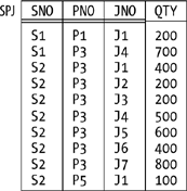
Let me put this point another way. To say that relvar R is in 5NF is to say that further nonloss decomposition of R into projections, while it might be possible, certainly won’t eliminate any redundancies. Note very carefully, however, that to say that R is in 5NF is not to say that R is redundancy-free. There are many kinds of redundancy that projection as such is powerless to remove—which is an illustration of the point I made earlier, in the section “The Place of Design Theory,” to the effect that there are numerous issues that design theory simply doesn’t address. By way of example, consider Figure 7-4, which shows a sample value for a relvar, SPJ, that’s in 5NF and yet suffers from redundancy. For example, the fact that supplier S2 supplies part P3 appears several times; so does the fact that part P3 is supplied to project J4—JNO stands for project number— and so does the fact that project J1 is supplied by supplier S2. (The relvar predicate is Supplier SNO supplies part PNO to project JNO in quantity QTY, and the sole key is {SNO,PNO,JNO}.) The only nontrivial join dependency satisfied by this relvar is this functional dependency:[*]
{ SNO, PNO, JNO } → { QTY }
which is an “arrow out of a superkey.” In other words, QTY depends on all three of SNO, PNO, and JNO, and it can’t appear in a relvar with anything less than all three. Hence, there’s no nonloss decomposition that can remove the redundancies.
There are a few further points I need to make here. First, I didn’t mention the point previously, but you probably know that 5NF is always achievable; that is, it’s always possible to decompose a non-5NF relvar into 5NF projections.
Second, every 5NF relvar is in BCNF, of course; so to say that R is in BCNF certainly doesn’t preclude the possibility that R is in 5NF as well. Informally, however, it’s very common to interpret statements to the effect that R is in BCNF as meaning that R is in BCNF and not in any higher normal form. I have not followed this practice in this chapter (and will continue not to do so).
Third, because it’s “the final normal form,” 5NF is sometimes called projection/join normal form (PJ/NF), to stress the point that it’s the normal form so long as we limit ourselves to projection as the decomposition operator and join as the recomposition operator. But I should immediately add that it’s possible to consider other operators and therefore, possibly, other normal forms. In particular, it’s possible, and desirable, to define (a) generalized versions of the projection and join operators, and hence (b) a generalized form of join dependency, and hence (c) a new “sixth” normal form, 6NF. It turns out that these developments are particularly important in connection with support for temporal data, and they’re discussed in detail in the book Temporal Data and the Relational Model by Hugh Darwen, Nikos Lorentzos, and myself (Morgan Kaufmann, 2003). However, all I want to do here is give a definition of 6NF that works for “regular” (that is, nontemporal) relvars. Here it is:
Definition: Relvar R is in 6NF if and only if it satisfies no nontrivial JDs at all.
Note in particular that a “regular” relvar is in 6NF if it consists of a single key, plus at most one additional attribute. Our usual shipments relvar SP is in 6NF, as is relvar SPJ (see Figure 7-4); by contrast, our usual suppliers and parts relvars S and P are in 5NF but not 6NF.
Note
A 6NF relvar is sometimes said to be irreducible, because it can’t be nonloss-decomposed via projection at all. Any 6NF relvar is necessarily in 5NF.
To close this subsection, observe that it follows from all of the above that any relvar that’s “all key” or consists of a key plus one additional attribute, since it’s in 6NF, is certainly in BCNF. However, it does not follow that such relvars are always well designed! For example, if relvar RS (see Figure 7-2) satisfies the FD {CITY} → {STATUS}, the projection of RS on {SNO,STATUS} is in BCNF—in fact, it’s in 6NF—but it certainly isn’t well designed. (See the discussion of dependency preservation in the section "Two Cheers for Normalization,” later, for a more detailed explanation.)
More on 5NF
Consider Figure
7-5, which shows a sample value for a simplified version of
relvar SPJ from the previous subsection. Suppose that simplified
version satisfies the join dependency ![]() {SP,PJ,SJ}, where SP, PJ, and SJ stand for
{SNO,PNO}, {PNO,JNO}, and {SNO,JNO}, respectively. What does that JD
mean from an intuitive point of view? The answer is as follows:
{SP,PJ,SJ}, where SP, PJ, and SJ stand for
{SNO,PNO}, {PNO,JNO}, and {SNO,JNO}, respectively. What does that JD
mean from an intuitive point of view? The answer is as follows:
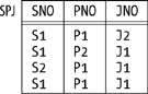
The JD means the relvar is equal to the join of, and so can be nonloss-decomposed into, its projections SP, PJ, and SJ. (Note that now I’m using the names SP, PJ, and SJ to refer to the projections as such, instead of to the corresponding subsets of the heading of relvar SPJ; I hope this kind of punning on my part doesn’t confuse you.)
It follows that the following constraint is satisfied:
  IF <
                     s,p
                     >
                     ∊ SP AND <
                     p,j
                     >
                     ∊ PJ AND <
                     s,j
                     >
                     ∊ SJ THEN <
                     s,p,j
                     >
                     ∊ SPJ
because if <s,p>, <p,j>, and <s,j> appear in SP, PJ, and SJ, respectively, then <s,p,j> certainly appears in the join of SP, PJ, and SJ, and that join is supposed to be equal to SPJ (that’s what the JD says). Given the sample value of Figure 7-5, for example, the tuples <S1,P1>, <P1,J1>, and <S1,J1> appear in SP, PJ, and SJ, respectively, and the tuple <S1,P1,J1> appears in SPJ. (I’m using what I hope is a self-explanatory shorthand notation for tuples, and I remind you that the symbol "∊" can be read as “appears in.”)
Now, the tuple <s,p> obviously appears in SP if and only if the tuple <s,p,z> appears in SPJ for some z. Likewise, the tuple <p,j> appears in PJ if and only if the tuple <x,p,j> appears in SPJ for some x, and the tuple <s,j> appears in SJ if and only if the tuple <s,y,j> appears in SPJ for some y. So the foregoing constraint is logically equivalent to this one:
  IF for some x
                     ,
                     y
                     ,
                     z
                     <s
                     ,
                     p
                     ,
                     z>
                     ∊ SPJ AND
                   <x
                     ,
                     p
                     ,
                     j>
                     ∊ SPJ AND
                   <s
                     ,
                     y
                     ,
                     j>
                     ∊ SPJ
  THEN             <s
                     ,
                     p
                     ,
                     j>
                     ∊ SPJ
With reference to Figure 7-5, for example, the tuples <S1,P1,J2>, <S2,P1,J1>, and <S1,P2,J1> all appear in SPJ, and therefore so does the tuple <S1,P1,J1>.
So the original JD is equivalent to the foregoing constraint. But what does that constraint mean in real-world terms? Well, here’s a concrete illustration. Suppose relvar SPJ contains tuples that tell us that all three of the following are true propositions:
Smith supplies monkey wrenches to some project.
Somebody supplies monkey wrenches to the Manhattan project.
Something is supplied to the Manhattan project by Smith.
Then the JD says the relvar must contain a tuple that tells us that the following is a true proposition too:
Smith supplies monkey wrenches to the Manhattan project.
Now, propositions 1, 2, and 3 together would normally not imply proposition 4. If we know only that propositions 1, 2, and 3 are true, then we know that Smith supplies monkey wrenches to some project (say, project z), that some supplier (say, supplier x) supplies monkey wrenches to the Manhattan project, and that Smith supplies some part (say, part y) to the Manhattan project—but we cannot validly infer that x is Smith or y is monkey wrenches or z is the Manhattan project. False inferences such as this one are examples of what’s sometimes called the connection trap . In the case at hand, however, the existence of the JD tells us there is no trap; that is, we can validly infer proposition 4 from propositions 1, 2, and 3 in this particular case.
Observe now the cyclic nature of the constraint (“IF s is connected to p and p is connected to j and j is connected back to s again, THEN s and p and j must all be directly connected, in the sense that they must all appear together in the same tuple”). It’s precisely if such a cyclic constraint occurs that we might have a relvar that’s in BCNF and not in 5NF. In my experience, however, such cyclic constraints are very rare in practice—which is why I said in the previous subsection that I don’t think they’re very important from a practical point of view.
I’ll close this section with a brief remark on fourth normal form (4NF). In the subsection “The Significance of 5NF,” I said that if you’re a database designer, you need to know about JDs and 5NF. In fact, you also need to know about multi-valued dependencies (MVDs) and fourth normal form. However, I mention these concepts for completeness only; like 2NF and 3NF, they’re mainly of historical interest. I’ll just note for the record that:
Details of what it means for an MVD to be trivial or implied by some superkey are beyond the scope of this discussion (see Exercise 7-19 at the end of the chapter)—but let me at least point out that it follows from these definitions that repeated nonloss-decomposition into exactly two projections is sufficient to take us at least as far as 4NF. By contrast, the JD in the previous subsection involved three projections, as I’m sure you noticed. In fact, we can say that in order to reach 5NF, decomposition into n projections (where n > 2) is necessary only if the relvar in question satisfies an n-way cyclic constraint: equivalently, only if it satisfies a JD involving n projections and not one involving fewer.
Two Cheers for Normalization
Normalization is far from being a panacea, as we can easily see by considering what its goals are and how well it measures up against them. Here are those goals:
To achieve a design that’s a “good” representation of the real world—one that’s intuitively easy to understand and is a good basis for future growth
To reduce redundancy
Thereby to avoid certain update anomalies
To simplify the statement and enforcement of certain integrity constraints
I’ll consider each in turn.
Good representation of the real world: Normalization does well on this one. I have no criticisms here.
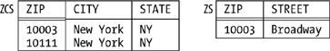
Reduce redundancy: Normalization is a good start on this problem, but it’s only a start. For one thing, it’s a process of nonloss decomposition, and (as we’ve seen) not all redundancies can be removed by nonloss decomposition; indeed, there are some kinds of redundancy, not discussed in this chapter so far, that normalization simply doesn’t address at all. For another thing, the objective of reducing redundancy can conflict with another objective, also not previously discussed—namely, the objective of dependency preservation . Let me explain. Consider the following relvar (attribute ZIP denotes ZIP Code or postcode):
ADDR { STREET, CITY, STATE, ZIP }
Assume for the sake of the example that this relvar satisfies the following FDs:
  { STREET, CITY, STATE } → { ZIP }
  { ZIP }                 → { CITY, STATE }
The second of these FDs implies that the relvar isn’t in BCNF. But if we apply Heath’s theorem and decompose it into BCNF projections as follows:
  ZCS { ZIP, CITY, STATE }
      KEY { ZIP }

  ZS { ZIP, STREET }
     KEY { ZIP, STREET }
then the FD {STREET,CITY,STATE} → {ZIP}, which was certainly satisfied by the original relvar, “disappears”! (It’s satisfied by the join of ZCS and ZS but, obviously enough, not by either of those projections alone.) As a consequence, relvars ZCS and ZS can’t be independently updated. For example, suppose those projections currently have values as shown in Figure 7-6; then an attempt to insert the tuple <10111,Broadway> into ZS will violate the “missing” FD. However, this fact can’t be determined without examining the projection ZCS as well as the projection ZS. For precisely this kind of reason, the dependency preservation objective says: Don’t split dependencies across projections.However, the ADDR example shows that, sadly, this objective and the objective of decomposing into BCNF projections can sometimes be in conflict.
Avoid update anomalies: This point is effectively just the previous one (“reduce redundancy”) by another name. It’s well known that less than fully normalized designs can be subject to certain update anomalies, precisely because of the redundancies they entail. In relvar STP, for example (see Figure 7-1 once again), supplier S1 might be shown as having status 20 in one tuple and status 25 in another. (Of course, this “update anomaly” can arise only if a less than perfect job is being done on integrity. Perhaps a better way to characterize the update anomaly issue is this: The constraints needed to prevent such anomalies are easier to state, and might be easier to enforce, if the design is fully normalized than they would be if it isn’t. See the next paragraph.)
Simplify statement and enforcement of constraints: It’s clear as a general observation that some constraints imply others. As a trivial example, if quantities must be less than or equal to 5000, they must certainly be less than or equal to 6000 (speaking a little loosely). Now, if constraint A implies constraint B, then stating and enforcing A will effectively state and enforce B “automatically” (indeed, B won’t actually need to be stated at all). And normalization to 5NF gives a very simple way of stating and enforcing certain important constraints: basically, all we have to do is define keys and enforce their uniqueness—which we’re going to do anyway—and then all JDs (and all MVDs and all FDs) will effectively be stated and enforced automatically, because they’ll all be implied by those keys. So normalization does a pretty good job in this area, too.
On the other hand . . . here are some more reasons why normalization is no panacea. First, JDs aren’t the only kind of constraint, and normalization doesn’t help with any others. Second, given a particular set of relvars, there’ll often be several possible decompositions into 5NF projections, and there’s little or no formal guidance available to tell us which one to choose in such cases. Third, there are many design issues that normalization simply doesn’t address at all. For example, what is it that tells us there should be just one suppliers relvar instead of one for London suppliers, one for Paris suppliers, and so on? It certainly isn’t normalization as classically understood.
That said, I must make it clear that I don’t want my comments in this section to be seen as an attack. I believe firmly that anything less than a fully normalized design is strongly contraindicated. In fact, I want to close this section with an argument—a logical argument, and one you might not have seen before—in support of the position that you should “denormalize” only as a last resort. That is, you should back off from a fully normalized design only if all other strategies for improving performance have somehow failed to meet requirements. By the way, note that I’m going along here with the usual assumption that normalization has performance implications. So it does, in current SQL products; but this is another topic I want to come back to later (see the section "Some Remarks on Physical Design“). Anyway, here’s the argument.
We all know that denormalization is bad for update (logically bad, I mean; it makes updates harder to formulate, and it can jeopardize the integrity of the database as well). What doesn’t seem to be so widely known is that denormalization can be bad for retrieval too; that is, it can make certain queries harder to formulate (equivalently, it can make them easier to formulate incorrectly—meaning, if they run, that you’re getting answers that might be “correct” in themselves but are answers to the wrong questions). Let me illustrate. Take another look at relvar RS (Figure 7-2), with its FD {CITY} → {STATUS}, and consider the query “Get the average city status.” Given the sample values in Figure 7-2, the status values for Athens, London, and Paris are 30, 20, and 30, respectively, and so the average is 26.667 (to three decimal places). Here are some attempts at formulating this query in SQL:
1 SELECT AVG ( RS.STATUS ) AS RESULT FROM RSResult(incorrect): 26. The problem here is that London’s status and Paris’s status have both been counted twice. Perhaps we need a DISTINCT inside the AVG invocation? Let’s try that:
2  SELECT AVG ( DISTINCT RS.STATUS ) AS RESULT
   FROM  RS
Result (incorrect): 25. No, it’s distinct cities we need to examine, not distinct status values. We can do that by grouping:
3  SELECT RS.CITY, AVG ( RS.STATUS ) AS RESULT
   FROM   RS
   GROUP  BY RS.CITY
Result (incorrect): <Athens,30>, <London,20>, <Paris,30>. This formulation gives average status per city, not the overall average. Perhaps what we want is the average of the averages?
4 SELECT RS.CITY, AVG ( AVG ( RS.STATUS ) ) AS RESULT FROM RS GROUP BY RS.CITYResult: Syntax error. The SQL standard quite rightly[*] doesn’t allow invocations of what it calls “set functions” such as AVG to be nested in this manner. One more attempt:
5  SELECT AVG ( TEMP.STATUS ) AS RESULT
   FROM ( SELECT DISTINCT RS.CITY, RS.STATUS
          FROM   RS ) AS TEMP
Result (correct at last): 26.667. As I pointed out in Chapter 5, however, not all SQL products allow nested subqueries to appear in the FROM clause in this manner.
That’s the end of normalization (for the time being, at any rate); now I want to switch to a topic that’s almost certainly less familiar to you, orthogonality , which constitutes another little piece of science in this overall business of database design.
Orthogonality
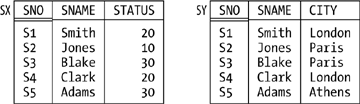
Figure 7-7 shows sample values for a possible but clearly bad design for suppliers: relvar SA is suppliers in Paris, and relvar SB is suppliers who either aren’t in Paris or have status 30. As you can see, the design leads to redundancy—to be specific, the tuple for supplier S3 appears in both relvars—and as usual such redundancies give rise to update anomalies. (Redundancy of any kind always has the potential to cause update anomalies.)

By the way, note that the tuple for supplier S3 must appear in both relvars. For suppose it appeared in SB but not SA, say. From SA, then, the Closed World Assumption would allow us to infer that it’s not the case that supplier S3 is in Paris. But SB tells us that supplier S3 is in Paris. Thus, we would have a contradiction on our hands, and the database would be inconsistent.
Well, the problem with the design of Figure 7-7 is obvious: it’s precisely the fact that the very same tuple can appear in two distinct relvars—meaning, more precisely, that it’s possible for that tuple to appear in both relvars without violating any constraint for either. So an obvious rule is:
The Principle of Orthogonal Design (first version): No two distinct relvars in the same database should be such that their relvar constraints permit the same tuple to appear in both.
The term orthogonal here derives from the fact that what the principle effectively says is that relvars should all be independent of one another—which they won’t be, if their constraints “overlap,” as it were.
Now, it should be clear that two relvars can’t possibly violate the foregoing principle if they’re of different types, and so you might be thinking the principle isn’t worth much. After all, it isn’t very usual for a database to contain two or more relvars of the same type. But consider Figure 7-8, which shows another possible but clearly bad design for suppliers. While there’s no way in that design for the same tuple to appear in both relvars, it is possible for a tuple in SX and a tuple in SY to have the same projection on {SNO,SNAME}[*]—and that fact leads to redundancy and update anomalies again. So we need to extend the design principle accordingly:
The Principle of Orthogonal Design (second and final version): Let A and B be distinct relvars in the same database. Then there must not exist nonloss decompositions of A and B into (say) A1, A2, . . . , Am and B1, B2, . . . , Bn, respectively, such that the relvar constraints for some projection Ai in the set A1, A2, . . . , Am and some projection Bj in the set B1, B2, . . . , Bn permit the same tuple to appear in both.
The term nonloss decomposition here refers to nonloss decomposition in the usual normalization sense.
Several points arise from the foregoing discussion and definition:
The second version of the principle subsumes the previous version, because one “nonloss decomposition” that’s always available for any relvar R is the one that consists of just the identity projection (the projection of R on all of its attributes).
Like the principles of normalization, The Principle of Orthogonal Design is basically just common sense—but (again like normalization) it’s formalized common sense.
The goal of orthogonal design is to reduce redundancy and thereby to avoid update anomalies (again like normalization). In fact, orthogonality complements normalization, in the sense that—loosely speaking—normalization reduces redundancy within relvars, while orthogonality reduces redundancy across relvars.
In fact, orthogonality complements normalization in another way, too. Again consider the decomposition of relvar S into its projections SX and SY, as illustrated in Figure 7-8. I now observe that that decomposition satisfies all of the usual normalization principles! Both projections are in 5NF; the decomposition is nonloss; dependencies are preserved; and both projections are needed to reconstruct the original relvar S.[*] It’s orthogonality, not normalization, that tells us the decomposition is bad.
Orthogonality might be common sense, but it’s often flouted in practice. That is, designs like this one, from a financial database, are encountered quite frequently:
  ACTIVITIES_2001 { ENTRYNO, DESCRIPTION, AMOUNT, NEW_BAL }
  ACTIVITIES_2002 { ENTRYNO, DESCRIPTION, AMOUNT, NEW_BAL }
  ACTIVITIES_2003 { ENTRYNO, DESCRIPTION, AMOUNT, NEW_BAL }
  ACTIVITIES_2004 { ENTRYNO, DESCRIPTION, AMOUNT, NEW_BAL }
  ACTIVITIES_2005 { ENTRYNO, DESCRIPTION, AMOUNT, NEW_BAL }
  ...
A better design involves just a single relvar:
ACTIVITIES { ENTRYNO, DESCRIPTION, AMOUNT, NEW_BAL, YEAR }Note
Of course, one reason why such multi-relvar designs occur in practice is because there are often good reasons for partitioning the data at the physical level, and the system in question is such that the partitioning therefore has to show through to the logical level as well. But reasons in favor of a certain physical design aren’t good reasons in favor of a bad logical design.
If A and B are relvars of the same type, adherence to the orthogonal design principle implies that:
                  A INTERSECT B
                  : is always empty
                  A UNION B
                  : is always a disjoint union

                  A MINUS B
                  : is always equal to A
Suppose we decide for some reason to decompose our usual suppliers relvar into a set of restrictions. Then orthogonality tells us those restrictions should be pairwise disjoint,in the sense that no tuple can ever appear in more than one of them. (Also, of course, the union of those restrictions must give us back the original relvar.) Such a decomposition is said to be an orthogonal decomposition .
Some Remarks on Physical Design
The relational model has nothing to say about physical design. But there are still some things that can usefully be said about physical design in a relational context—things that are at least implied by the model, even though they aren’t stated explicitly (and even though the details of physical design are, of necessity, somewhat DBMS-specific and vary from system to system).
The first point is that physical design should follow logical design. That is, the “right” approach is to do a clean logical design first, and then, as a follow-on step, to map that logical design into whatever physical structures the target DBMS happens to support. Equivalently, the physical design should be derived from the logical design and not the other way around. Ideally, in fact, the system should be able to derive an optimal physical design for itself, without any need for human involvement at all. (This goal isn’t as far-fetched as it might sound. I’ll say a little more about it later in this section.)
As for my second point: we saw in Chapter 1 that one reason for excluding physical issues of all kinds from the relational model was to give implementers the freedom to implement the model in any way they liked—and here, I think, the widespread lack of understanding of the model has really hurt us. Certainly most SQL products have failed to live up to the model’s full potential in this respect; in those products, what the user sees and what’s physically stored are essentially the same thing. In other words, what’s physically stored is effectively just a direct image of what the user logically sees, as Figure 7-9 suggests. (I realize these remarks are oversimplified, but they’re true enough for present purposes.)

Now, there are many things wrong with this direct-image style of implementation, far too many to discuss in detail here. But the overriding point is that it provides almost no data independence: if we have to change the physical design (for performance reasons, of course), we have to change the logical design too. In particular, it accounts for the argument, so often heard, to the effect that we have to “denormalize for performance.” In principle, logical design has absolutely nothing to do with performance at all; but if the logical design maps one-to-one to the physical design . . . well, the conclusion is obvious. Surely we can do better than this. Relational advocates have argued for years that the relational model doesn’t have to be implemented this way. And indeed it doesn’t; all being well, a brand-new implementation technology is due to appear soon that addresses all of the problems of the direct-image scheme. That technology is called The TransRelational? Model. Since it is an implementation technology, the details are beyond the scope of this book; you can find a preliminary description in my book An Introduction to Database Systems, Eighth Edition (Addison-Wesley, 2004). All I want to do here is point out a few desirable consequences of having an implementation that does keep the logical and physical levels rigidly and properly separate.
First, we would never need to “denormalize for performance” at all (at the logical level, I mean); all relvars could be in 5NF, or even 6NF, without any performance penalty. The logical design really would have no performance implications at all.
Second, 6NF offers a basis for a truly relational way of dealing with the problem of missing information (I mean, a way that doesn’t involve nulls and three-valued logic). If you use nulls, you’re effectively making the database state explicitly that there’s something you don’t know. But if you don’t know something, it’s much better to say nothing at all! To quote Wittgenstein: Wovon man nicht reden kann, darüber muss man schweigen (“Whereof one cannot speak, thereon one must remain silent”). For example, suppose for simplicity that there are just two suppliers right now, S1 and S2, and we know the status for S1 but not for S2. A 6NF design for this situation might look as shown in Figure 7-10.
Of course, there’s a lot more that could and should be said about this approach to missing information, but this isn’t the place. Here I just want to stress the point that with this design, we don’t have a “tuple” showing supplier S2’s status as “null”—we don’t have a tuple showing supplier S2’s status at all.
Finally, in the kind of system I’m sketching here, it really would be possible for the system to derive the optimal physical design from the logical design automatically, with little or no involvement on the part of any human designer. Space considerations among other things mean I can’t provide evidence here to support this claim, but I stand by it.
Summary
The main focus of this chapter has been on logical database design theory, by which I mean, essentially, normalization and orthogonality (the scientific part of the design discipline). The point is that logical design, unlike physical design, is or should be quite DBMS-independent, and as we’ve seen there are some solid theoretical principles that can usefully be applied to the problem.
One point I didn’t call out explicitly in the body of the chapter is that logical design should generally aim to be application-independent, too, as well as DBMS-independent. The aim is to produce a design that concentrates on what the data means, rather than on how it will be used— and I emphasized the significance of constraints and predicates (“business rules”) in this connection. The database is supposed to be a faithful representation of the semantics of the situation, and constraints are what represent semantics. Abstractly, then, the logical design process goes like this:
Pin down the relvar predicates as carefully as possible.
Map the output from Step 1 into relvars and constraints. Of course, some of those constraints will be FDs, MVDs, or JDs in particular.
Incidentally, one reason application independence is desirable is that we never know all of the uses to which the data will be put. It follows that we want a design that will be robust, one that won’t be invalidated by new processing requirements.
Much of design theory has to do with reducing redundancy: normalization reduces redundancy within relvars, orthogonality reduces it across relvars. My discussion of normalization concentrated on BCNF and 5NF, which are the normal forms with respect to FDs and JDs, respectively. (However, I did at least mention other normal forms, including 6NF in particular.) I pointed out that normalization makes certain constraints easier to state (and perhaps enforce); equivalently—this is something else I didn’t say earlier—it makes more single-tuple updates logically acceptable than would otherwise be the case (because unnormalized designs imply redundancy, and redundancy implies that sometimes we have to update several things at once). I explained that normalization is really formalized common sense. I also gave a logical and possibly unfamiliar argument, having to do with retrieval rather than update, for not denormalizing; here let me add that although the cry is always “denormalize for performance,” denormalization can actually be bad for performance (both retrieval and update performance, too), as you probably know. In fact, “denormalizing for performance” usually means improving the performance of one application at the expense of others.
I also described The Principle of Orthogonal Design (more formalized common sense), and I offered a few remarks on physical design. First, the physical design should be derived from the logical design and not the other way around. Second, it would be nice to get away from the currently ubiquitous direct-image style of implementation. Third, it would also be nice if physical design could be fully automated, and I held out some hope in this regard.
One last point: I want to stress that the principles of normalization and orthogonality are always, in a sense, optional. They aren’t hard and fast rules, never to be broken. As we know, sometimes there are sound reasons for not normalizing “all the way” (sound logical reasons, I mean; I’m not talking about “denormalizing for performance”). Well, the same is true of orthogonality—although, just as a failure to normalize all the way implies redundancy and can lead to certain anomalies, so too can a failure to adhere to orthogonality. Even with the design theory I’ve been describing in this chapter, database design usually involves trade-offs and compromises.
Exercises
Exercise 7-1
Give definitions, as precisely as you can, of functional dependency and join dependency.
Exercise 7-2
List all of the FDs, trivial as well as nontrivial, satisfied by our usual shipments relvar SP.
Exercise 7-3
The concept of FD relies on the notion of tuple equality: true or false?
Exercise 7-4
Prove Heath’s theorem. Prove also that the converse of that theorem isn’t valid.
Exercise 7-5
Nonloss decomposition means a relvar is decomposed into projections in such a way that we can recover the original relvar by joining those projections back together again. In fact, if projections r1 and r2 of relation r are such that every attribute of r appears in at least one of r1 and r2, then joining r1 and r2 will always produce every tuple of r. Prove this assertion. (It follows from the foregoing that the problem with a lossy decomposition is that the join produces additional, “spurious” tuples. Since we have no way in general of knowing which tuples in the result are spurious and which genuine, we’ve lost information.)
Exercise 7-6
What’s a superkey? What does it mean to say an FD is implied by a superkey? What does it mean to say a JD is implied by a superkey?
Exercise 7-7
Keys are supposed to be unique and irreducible. Now, the system is obviously capable of enforcing uniqueness; but what about irreducibility?
Exercise 7-8
What’s (a) a trivial FD, (b) a trivial JD? Is the former a special case of the latter?
Exercise 7-9
Let R be a relvar of degree n. What’s the maximum number of FDs that R can possibly satisfy (trivial as well as nontrivial)?
Exercise 7-10
Given that A and B in the FD A → B are both sets of attributes, what happens if either is the empty set?
Exercise 7-11
Here’s a predicate: on day d during period p, student s is attending lesson l, which is being taught by teacher t in classroom c (where d is a day of the week—Monday to Friday—and p is a period—1 to 8—within the day). Lessons are one period in duration and have a name that’s unique with respect to all lessons taught in the week. Design a set of BCNF relvars for this database. Are your relvars in 5NF? 6NF? What are the keys?
Exercise 7-12
Most of the examples of nonloss decomposition in the body of the chapter showed a relvar being decomposed into exactly two projections. Is it ever necessary to decompose into three or more?
Exercise 7-13
Many database designers recommend the use of artifical or surrogate keys in base relvars in place of what are sometimes called “natural” primary keys. For example, we might add an attribute—SPNO, say—to our usual shipments relvar (making sure it has the uniqueness property, of course) and then make {SPNO} a surrogate primary key for that relvar. (Note, however, that {SNO,PNO} would still be a key; it just wouldn’t be the primary key any longer.) Thus, surrogate keys are keys in the usual relational sense, but (a) they always involve exactly one attribute and (b) their values serve solely as surrogates for the entities they stand for (that is, they serve merely to represent the fact that those entities exist—they carry absolutely no additional meaning or baggage of any kind). Ideally, those surrogate values would be system-generated, but whether they’re system- or user-generated has nothing to do with the basic idea of surrogate keys as such. Are surrogate keys the same thing as tuple IDs? And do you think they’re a good idea?
Exercise 7-14
(With acknowledgments to Hugh Darwen.) I decided to throw a party, so I drew up a list of people I wanted to invite and made some preliminary soundings. The response was good, but several people made their acceptance conditional on the acceptance of certain other invitees. For example, Bob and Cal both said they would come if Amy came; Hal said he would come if either Don and Eve both came or Fay came; Guy said he would come anyway; Joe said he would come if Bob and Amy both came; and so on. Design a database to show whose acceptance is based on whose.
Exercise 7-15
Design a database for the following. The entities to be represented are employees and programmers. Every programmer is an employee, but some employees aren’t programmers. Employees have an employee number, name, and salary. Programmers have a (single) programming language skill. What difference would it make if programmers could have an arbitrary number of such skills?
Exercise 7-16
Let A, B,and C be subsets of the heading of relvar R such that the (set-theoretic) union of A, B, and C is equal to that heading. Let AB denote the (set-theoretic) union of A and B,and similarly for AC. Then R satisfies the multi-valued dependencies (MVDs):
  A
                  →
                  →
                  B

  A
                  →
                  →
                  C
(where A → → B is pronounced
"A double arrow B" or
"A multi-determines B" or
"B is multi-dependent on
A,” and similarly for A
→ → C) if and only if
R satisfies the JD ![]() {AB,AC}. Show that if
relvar R satisfies the MVDs
A → → B and
A → → C, then it satisfies
the property that if it includes the pair of tuples
<a,b1,c1> and
<a,b2,c2>, then it also includes the pair
of tuples <a,b1,c2> and
<a,b2,c1>.
{AB,AC}. Show that if
relvar R satisfies the MVDs
A → → B and
A → → C, then it satisfies
the property that if it includes the pair of tuples
<a,b1,c1> and
<a,b2,c2>, then it also includes the pair
of tuples <a,b1,c2> and
<a,b2,c1>.
Exercise 7-17
Show that if R satisfies the FD A → B, it also satisfies the MVD A → → B.
Exercise 7-18
(Fagin’s theorem.) Let R be as in Exercise 7-16. Show that R can be nonloss-decomposed into its projections on AB and AC if and only if it satisfies the MVDs A → → B and A → → C.
Exercise 7-19
Show that if K is a key for R, then K → → A is satisfied for all attributes A of R.
Note
Here is a convenient place to introduce some more definitions. Recall that R is in 4NF if and only if every nontrivial MVD it satisfies is implied by some superkey. The MVD A → → B is trivial if and only if AB is equal to the heading of R or A is a superset of B; it’s implied by a superkey if and only if A is a superkey.
Exercise 7-20
Give an example of a relvar that’s in BCNF and not 4NF.
Exercise 7-21
Design a database for the following. The entities to be represented are sales representatives, sales areas, and products. Each representative is responsible for sales in one or more areas; each area has one or more responsible representatives. Each representative is responsible for sales of one or more products, and each product has one or more responsible representatives. Each product is sold in each area; however, no two representatives sell the same product in the same area. Each representative sells the same set of products in each area for which that representative is responsible.
Exercise 7-22
Write a Tutorial D CONSTRAINT statement to express the JD satisfied by relvar SPJ of Figure 7-5.
Exercise 7-23
(Modified version of Exercises 7-27.) Design a database for the following. The entities to be represented are sales representatives, sales areas, and products. Each representative is responsible for sales in one or more areas; each area has one or more responsible representatives. Each representative is responsible for sales of one or more products, and each product has one or more responsible representatives. Each product is sold in one or more areas, and each area has one or more products sold in it. Finally, if representative r is responsible for area a, product p is sold in area a, and representative r sells product p, then r sells p in a.
Exercise 7-24
Which of the following are true statements?
Every “all key” relvar is in BCNF.
Every “all key” relvar is in 5NF.
Every binary relvar is in BCNF.
Exercise 7-25
There’s a lot of discussion in the industry at the time of writing about the possibility of XML databases. But XML documents are inherently hierarchic in nature. Do you think the criticisms of hierarchies in the body of the chapter apply to XML databases? Justify your answer.
Exercise 7-26
Draw E/R diagrams for the databases from Exercises 7-11,7-14 7-21, and 7-23. What do you conclude from this exercise?
Exercise 7-27
A certain database includes two base relvars that look like this:
  FATHER_OF { X NAME, Y NAME } KEY { X }
  MOTHER_OF { X NAME, Y NAME } KEY { X }
The predicates are The father of X is Y and The mother of X is Y, respectively. For simplicity, no constraints are defined, except for the two KEY constraints. Comment on this design.
Exercise 7-28
This chapter has been concerned with data design; in essence, I’ve discussed certain aspects of relational design, and there’s a strong argument that you should do a clean relational design first, even if your target DBMS isn’t relational at all. In the same kind of way, it’s sometimes suggested that transaction or query design might be done by defining the transaction or query in terms of relational algebra first, and then mapping that definition into SQL (or whatever your target language is) as a follow-on activity afterward. What do you think of this strategy?
[*] It’s also, in this particular example, an implied constraint (as it was before, in fact, since it was implied by the constraint KEY{SNO} for RS). To be specific, it’s implied by the combination of constraints KEY{SNO} (for SNC), KEY{CITY} (for CS), and the foreign key constraint from SNC to CS.
[*] In earlier chapters I said it was relations, not relvars, that were always in 1NF, but no harm is done if we extend the term to apply to relvars as well.
[*] Equivalently, using the name SPJQ to refer to the set of all
attributes of SPJ, the relvar satisfies the trivial JD
![]() {SPJQ}. (Recall from Chapter 5 that the join of a
single relation r is just
r itself.)
{SPJQ}. (Recall from Chapter 5 that the join of a
single relation r is just
r itself.)
[*] I say “quite rightly” only because we’re in the SQL context specifically; a more orthodox language would certainly let us nest such invocations. Let me explain. Consider the SQL expression SELECT SUM(SP.QTY) AS SQ FROM SP WHERE SP.QTY > 100 (I deliberately switch to a different example). The SUM argument here is really SP.QTY FROM SP WHERE SP.QTY > 100, and a more orthodox language would therefore enclose that whole expression in parentheses. But SQL doesn’t. As a consequence, an expression of the form AVG(SUM(QTY)) has to be illegal, because SQL can’t figure out which portions of the rest of the surrounding expression are part of the AVG argument and which are part of the SUM argument.
[*] Projection is a relational operator, of course, but it clearly makes sense to define a version of the operator that works for tuples instead of relations and thereby to talk of a projection of some tuple. A similar remark applies to several other relational operators, too.
[*] I said earlier that a decomposition is nonloss if, when we join the projections back together, we get back to the original relvar. That’s true, but it’s not quite enough; in practice, we surely want to impose the extra requirement that every projection is needed in that join. For example, we probably wouldn’t consider the decomposition of relvar S into its projections on {SNO}, {SNO,STATUS}, and {SNO,SNAME,CITY} as a sensible design—yet S is certainly equal to the join of those three projections.