
Chapter Five. Relational Algebra
I’ll begin this chapter by briefly reviewing a few important points from Chapter 1 . First, I remind you that each algebraic operator takes at least one relation as input and produces another relation as output. Second, I remind you that the fact that the output is the same kind of thing as the input—they’re all relations—is the closure property of the algebra, and it’s that property that lets us write nested relational expressions. Third, I gave outline descriptions in Chapter 1 of what I called "the original eight operators" (restrict, project, product, intersect, union, difference, join, and divide); now I want to define those operators, as well as a number of others, much more carefully. Before I can do so, however, I need to make a few general points:
First, the operators are generic: they apply, in effect, to all possible relations. For example, we don’t need one specific join operator to join employees and departments and another, different, join operator to join suppliers and shipments. (Incidentally, do you think an analogous observation applies to object-oriented systems?)
Second, the operators are read-only: they “read” their operands and return a result, but they don’t update anything. In other words, they operate on relations, not relvars.
Of course, the previous point doesn’t mean that relational expressions can’t refer to relvars. For example, R UNION S, where R and S are relvar names, is certainly a valid relational expression in Tutorial D. In the context of such an expression, however, a relvar name doesn’t denote the corresponding relvar as such; rather, it denotes the relation that happens to be the current value of that relvar at that time. In other words, we can certainly use a relvar name to denote a relation operand, and such a relvar reference thus constitutes a valid relational expression[*]—but in principle we could equally well denote the very same operand by means of an appropriate relation literal instead. (An analogy might help clarify this point. Suppose N is a variable of type INTEGER, and at time t it has the value 3. Then N+2 is certainly a valid expression, but at time t it means exactly the same as 3+2, no more and no less.)
Last, given that the operators of the algebra are all read-only, it follows that INSERT, DELETE, and UPDATE (and relational assignment), though they are relational operators, aren’t part of the algebra as such.
I also need to say something about the design of Tutorial D, because its support for the algebra differs in certain significant respects from that of SQL (perhaps it would be more accurate to say that its support for the algebra is—deliberately, of course—much more direct than that of SQL). The overriding point is that, in operations such as UNION or JOIN that need some correspondence to be established between operand attributes, Tutorial D does so by requiring the attributes in question to have the same names (as well as, necessarily, the same types). For example, here’s a Tutorial D expression for the join of parts and suppliers on cities:
P JOIN S
By definition, this join is performed on the basis of part and supplier cities, P and S having just the CITY attribute in common. Here by contrast is the same operation in SQL (note the last line in particular):
  SELECT P.PNO, P.PNAME, P.COLOR, P.WEIGHT, P.CITY,
       S.SNO, S.SNAME, S.STATUS
  FROM   P,S
  WHERE  P.CITY = S.CITY
Note: Actually, this example can be formulated in many different ways in SQL, and here are three more. As you’ll observe, the second and third are a little closer to the spirit of Tutorial D (note in particular that the result of the join in those two formulations has a column called just CITY and no columns called either S.CITY or P.CITY):
  SELECT P.PNO, P.PNAME, P.COLOR, P.WEIGHT, P.CITY,
       S.SNO, S.SNAME, S.STATUS
  FROM   P JOIN S
  ON   P.CITY = S.CITY

  SELECT P.PNO, P.PNAME, P.COLOR, P.WEIGHT, CITY,
       S.SNO, S.SNAME, S.STATUS
  FROM   P JOIN S
  USING  ( CITY )

  SELECT P.PNO, P.PNAME, P.COLOR, P.WEIGHT, CITY,
       S.SNO, S.SNAME, S.STATUS
  FROM   P NATURAL JOIN S
I chose the particular formulation I did partly because it was the only one supported in SQL as originally defined and partly, and more importantly, because it allows me to make a number of additional points concerning differences between SQL and the algebra (at least as realized in Tutorial D):
SQL permits (and sometimes requires) dot-qualified names. Tutorial D doesn’t.
Tutorial D sometimes needs to rename attributes in order to avoid what would otherwise be naming clashes or mismatches. SQL usually doesn’t (though it does support an analog of the RENAME operator that Tutorial D uses for the purpose, as we’ll see in the next section).
Partly as a consequence of the previous point, Tutorial D has no need for SQL’s “correlation names” (in effect, it replaces SQL’s correlation-name concept by the idea that attributes occasionally need to be renamed in order to “disambiguate” what would otherwise be a syntactically invalid expression).
In addition to either explicitly or implicitly supporting certain features of the relational algebra, SQL also explicitly supports certain features of the relational calculus (EXISTS is a case in point—see Appendix A). Tutorial D doesn’t. One consequence of this difference is that SQL tends to be a rather redundant language, in that it often provides numerous different ways of formulating the same query (a fact that can have serious negative implications for the optimizer).[*]
SQL requires most queries to conform to its SELECT - FROM - WHERE template. Tutorial D has no analogous requirement. I’ll have more to say on this particular issue in the section Extend and Summarize,” later in this chapter.
In what follows, I’ll show most examples in both Tutorial D and SQL.
More on Closure
When I say the output from each algebraic operation is another relation, I hope it’s clear that I’m talking from a conceptual point of view. I don’t mean the system actually has to materialize that output in its entirety. For example, consider the following expression (a restriction of a join—Tutorial D on the left, SQL on the right):
  ( P JOIN S )             |  SELECT P.*,
  WHERE PNAME > SNAME   |     S.SNO, S.SNAME, S.STATUS
                           |  FROM   P, S
                           |  WHERE  P.CITY = S.CITY
                           |  AND  P.PNAME > S.SNAME
Clearly, as soon as a given tuple of the join is formed, the system can test that tuple right away against the restriction condition PNAME > SNAME (P.PNAME > S.SNAME in the SQL version) to see if it belongs in the final output and discard it if not. Thus, the intermediate result that’s the output from the join might never exist as a fully materialized relation in its own right at all. (In fact, of course, the system tries very hard not to materialize intermediate results in their entirety, for obvious performance reasons.)
The foregoing example raises another important point, however. Consider the boolean expression PNAME > SNAME in the Tutorial D version. That expression applies, conceptually, to the result of P JOIN S, and the attribute names PNAME and SNAME in that expression therefore refer to attributes of that result—not to the attributes of those names in relvars P and S. But how do we know the result includes any such attributes? What is the heading of that result? More generally, how do we know what the heading is for the result of any algebraic operation? Clearly, what we need is a set of inference rules— to be more specific, relation type inference rules— such that if we know the type(s) of the input relation(s) for any given operation, we can infer the type of the output relation from that operation. In the case of join, for example, those rules say the output from P JOIN S is of this type:
  RELATION { PNO PNO, PNAME NAME, COLOR COLOR, WEIGHT WEIGHT,
             CITY CHAR, SNO SNO, SNAME NAME, STATUS INTEGER }
In fact, for join, the heading of the output is the union of the headings of the inputs—where by union I mean the regular set-theoretic union, not the special relational union I’ll be discussing later in this chapter. In other words, the output has all of the attributes of the inputs, except that common attributes—just CITY in the example—appear once, not twice. Of course, those attributes don’t have any left-to-right order, so I could equally well say that (for example) the type of the result of P JOIN S is this:
  RELATION { SNO SNO, PNO PNO, SNAME NAME, PNAME NAME, CITY CHAR,
             STATUS INTEGER, WEIGHT WEIGHT, COLOR COLOR }
Note that type inference rules of some kind are definitely needed in order to support the closure property fully. Closure says that every result is a relation, and relations have not just a body but also a heading; thus, every result must have a proper relational heading as well as a proper relational body.
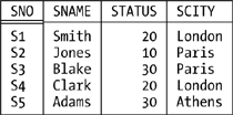
The RENAME operator mentioned in this chapter’s introduction is needed in large part to support the relational model’s type inference rules. RENAME takes one relation as input and returns another relation as output; the output relation is identical to the input relation, except that one of its attributes has a different name. For example (Tutorial D on the left and SQL on the right):
  S RENAME ( CITY AS SCITY )  | SELECT S.SNO, S.SNAME, S.STATUS,
                              |        S.CITY AS SCITY
                              | FROM   S
Given our usual sample values, the result looks like this:
(I won’t usually bother to show results explicitly in this chapter unless I think the particular operator I’m talking about might be unfamiliar to you, as in the case at hand.)
Note
Important: The foregoing example does not change relvar S in the database! RENAME isn’t like SQL’s ALTER TABLE; the RENAME invocation is only an expression (just as, for example, P JOIN S or N+2 are only expressions), and like any expression it simply denotes a certain value. What’s more, of course, since it is an expression, not a statement or “command,” it can be nested inside other expressions. We’ll see plenty of examples later.
So how does SQL handle this business of specifying result attribute names (or column names, rather)? The answer is: not very well. First of all, we saw in Chapter 3 that SQL doesn’t really have a notion of “relation type” anyway (it has row types instead). Second, it can produce results with columns that effectively have no name at all (for example, consider SELECT DISTINCT P.WEIGHT * 2 FROM P). Third, it can also produce results with duplicate column names (for example, consider SELECT DISTINCT P.CITY, S.CITY FROM P, S). Finally, let’s take another look at the example from the beginning of this section:
  ( P JOIN S )             |  SELECT P.*,
  WHERE PNAME > SNAME   |     S.SNO, S.SNAME, S.STATUS
                           |  FROM   P, S
                           |  WHERE  P.CITY = S.CITY
                           |  AND  P.PNAME > S.SNAME
As you can see, the counterpart to Tutorial D’s PNAME > SNAME in the SQL version is P.PNAME > S.SNAME—which is curious, because that expression is supposed to apply to the result of the FROM clause, and relvars P and S certainly aren’t part of that result! Indeed, it’s quite difficult to explain how something like P.PNAME in the WHERE and SELECT clauses (and possibly elsewhere in the overall expression) can make any sense at all in terms of the result of the FROM clause. The SQL standard does explain it, but the machinations it has to go through in order to do so are much more complicated than Tutorial D’s rules—so much so that I won’t even try to explain them here, but will simply rely on the fact that they can be explained if necessary. I justify the omission by appealing to the fact that this book is supposed to be about the relational model, not SQL.
Now I’d like to go on to describe some other algebraic operators. Please note that I’m not trying to be exhaustive in what follows; I won’t be covering “all known operators,” and I won’t even define all of the operators I do cover in full generality. In most cases, in fact, I’ll just give a careful but somewhat informal definition and show some simple examples.
The Original Operators
This section gives definitions for the original set of relational operators defined by Codd: restrict, project, join, intersect, union, difference, product, and divide.
Restrict
Let bx be a boolean expression involving zero or more attribute names, such that all of the attributes mentioned are attributes of the same relation r.[*] Then the restriction of r according to bx:
r WHERE bx
is a relation with a heading the same as that of r and a body consisting of all tuples of r for which bx evaluates to TRUE. For example:
  S WHERE CITY = 'Paris'  | SELECT S.*
                          | FROM   S
                          | WHERE  S.CITY = 'Paris'
As an aside, I remark that restrict is sometimes called select; I prefer not to use this term, however, because of the potential confusion with SQL’s SELECT.
Project
Let relation r have attributes X, Y,. . . , Z (and possibly others). Then the projection of r on X, Y, . . . , Z:
r { X, Y, ..., Z }
is a relation with (a) a heading derived from the heading of r by removing all attributes not mentioned in the set {X,Y, . . . ,Z} and (b) a body consisting of all tuples {X x,Y y, . . . ,Z z} such that a tuple appears in r with X value x, Y value y, . . ., and Z value z. For example:
  S { SNAME, CITY, STATUS }  | SELECT DISTINCT S.SNAME,
                             |        S.CITY, S.STATUS
                             | FROM   S
To repeat, the result is a relation; thus, “duplicates are eliminated,” to use the common phrase, and that DISTINCT in the SQL formulation is really needed, therefore.
By the way, Tutorial D also allows a projection to be expressed in terms of the attributes to be discarded instead of the ones to be kept. Thus, for example, the Tutorial D expressions:
S { SNAME, CITY, STATUS }
and:
S { ALL BUT SNO }
are equivalent. This feature can save a lot of writing (think of projecting a relation of degree 100 on 99 of its attributes). An analogous remark applies to SUMMARIZE (BY form only) and GROUP (see the later sections "Extend and Summarize" and "Group and Ungroup,” respectively).
In concrete syntax, it turns out to be convenient to assign high precedence to the projection operator. In Tutorial D, for example, we take this expression:
S JOIN P { PNO, CITY }
to mean:
S JOIN ( P { PNO, CITY } )
and not:
( S JOIN P ) { PNO, CITY }
As an exercise, show the difference between these two interpretations, given our usual sample data.
Join
Let relations r and s have attributes X1, X2, . . . , Xm, Y1, Y2, ..., Yn and Y1, Y2, . . . , Yn, Z1, Z2, . . . , Zp, respectively; in other words, the Y’s (n of them) are the common attributes, the X’s (m of them) are the other attributes of r, and the Z’s (p of them) are the other attributes of s. We can assume without loss of generality that none of the X’s has the same name as any of the Z’s, thanks to the availability of RENAME. Now let the X’s taken together be denoted just X, and similarly for the Y’s and the Z’s. Then the natural join [*] (join for short) of r and s:
r JOIN s
is a relation with (a) a heading that is the (set-theoretic) union of the headings of r and s and (b) a body consisting of the set of all tuples t such that t is the (set-theoretic) union of a tuple appearing in r and a tuple appearing in s. In other words, the heading is {X,Y,Z} and the body consists of all tuples {X x,Y y,Z z} such that a tuple appears in r with X value x and Y value y and a tuple appears in s with Y value y and Z value z. Here again is the example from the introductory section:
  P JOIN S  | SELECT P.PNO, P.PNAME, P.COLOR, P.WEIGHT, P.CITY,
            |        S.SNO, S.SNAME, S.STATUS
            | FROM   P, S
            | WHERE  P.CITY = S.CITY
Now, I’m quite sure you were already familiar with what I’ve said so far regarding join, but you might not be so familiar with the following points. First of all, I remind you that the SQL standard allows the join of parts and suppliers on cities to be expressed in an alternative style that’s a little closer to that of Tutorial D (and this time I deliberately replace that long list of column references in the SELECT clause by a simple “*”):
  SELECT *
  FROM   P NATURAL JOIN S
However, not all SQL products actually support this syntax.
Second, and more important, intersection is a special case of join. To be specific, if m = p = 0 (meaning there are no X’s and no Z’s, and r and s are thus of the same type), r JOIN s degenerates to r INTERSECT s (see the next subsection "Intersect“).
Third (also important), cartesian product is a special case of join, too: if n = 0, meaning there are no Y’s and r and s thus have no common attributes at all, r JOIN s degenerates to r TIMES s (see the later subsection "Cartesian Product“). Why? Because (a) the set of attributes common to r and s in this case is the empty set of attributes; (b) every possible tuple has the same value for the empty set of attributes (namely, the 0-tuple); thus, (c) every tuple in r joins to every tuple in s, and so we get the cartesian product as stated.
Fourth, it turns out in practice that many queries that require join really require an extended form of that operator called semijoin . (You might not have heard of semijoin before, but in fact it’s quite important.) Here’s the definition: the semijoin of r with s is the join of r and s, projected back on to the attributes of r. By way of example, consider the query “Get suppliers who supply at least one part”:
  S SEMIJOIN SP  | SELECT DISTINCT S.*
                 | FROM   S, SP
                 | WHERE  S.SNO = SP.SNO
As you can see, this query can be thought of as asking for just those suppliers that match at least one shipment. Tutorial D therefore provides a more user-friendly spelling for SEMIJOIN that allows the query to be expressed thus:
S MATCHING SP
Now observe what happens to r JOIN s if p = 0 (meaning the heading of s is a subset of that of r-- equivalently, every attribute of s is an attribute of r). As I hope you can see, r JOIN s degenerates to r MATCHING s in this case. Likewise, if m = 0, r JOIN s degenerates to s MATCHING r (note that r MATCHING s and s MATCHING r are different, in general).
Fifth, join is fundamentally a dyadic operator, meaning it takes two operands. However, it’s possible, and useful, to support an n-adic or prefix version of the operator (and Tutorial D does), according to which we can write expressions of the form:
JOIN { r, s, ..., w }
to join any number of relations r, s, . . . ,w. For example, the join of parts and suppliers could alternatively be expressed as follows:
JOIN { P, S }
What’s more, we can use this syntax to ask for “joins” of just a single relation, or even of no relations at all! The join of a single relation, JOIN{r}, is just r itself; this case is perhaps not of much practical importance. Perhaps surprisingly, however, the join of no relations at all, JOIN{}, is very important indeed!—and the result is TABLE_DEE. (Recall that TABLE_DEE is the unique relation with no attributes and one tuple.) Why is the result TABLE_DEE? Well, consider the following:
In ordinary arithmetic, 0 is the identity with respect to “+”; that is, for all numbers x, the expressions x + 0 and 0 + x are both identically equal to x. As a consequence, the sum of no numbers is 0. (To see that this claim is reasonable, consider a piece of code that computes the sum of n numbers by initializing the sum to 0 and then iterating over those n numbers. What happens if n = 0?)
In like manner, 1 is the identity with respect to “*”; that is, for all numbers x, the expressions x * 1 and 1 * x are both identically equal to x. As a consequence, the product of no numbers is 1.
In the relational algebra, TABLE_DEE is the identity with respect to JOIN; that is, the join of any relation r with TABLE_DEE is simply r. As a consequence, the join of no relations is TABLE_DEE.
If you’re having difficulty with this idea, don’t worry about it too much for now. But if you come back to reread this section later, I suggest you try to convince yourself then that r JOIN TABLE_DEE and TABLE_DEE JOIN r are indeed both identically equal to r. It might help if I point out that the joins in question are actually cartesian products (right?).
Intersect
Let relations r and s be of the same type. Then the intersection of those relations, r INTERSECT s, is a relation of the same type, with a body consisting of all tuples t such that t appears in both r and s. For example:
  S { CITY }    | SELECT DISTINCT S.CITY
    INTERSECT   | FROM   S
    P { CITY }  | INTERSECT
                | SELECT DISTINCT P.CITY
                | FROM   P
(Actually we don’t need those DISTINCTs in the SQL version, but I prefer to include them for explicitness. See the upcoming discussion of union.)
As we’ve already seen, intersect is really just a special case of join. Tutorial D and SQL both support it, however, if only for psychological reasons. Tutorial D also supports an n-adic or prefix form, but I’ll skip the details here.
Union
Again, let relations r and s be of the same type. Then the union of those relations, r UNION s, is a relation of the same type, with a body consisting of all tuples t such that t appears in r or s or both. For example:
  S { CITY } UNION P { CITY }  | SELECT DISTINCT S.CITY
                               | FROM   S
                               | UNION  DISTINCT
                               | SELECT DISTINCT P.CITY
                               | FROM   P
As with projection, it’s worth noting explicitly in connection with union that “duplicates are eliminated.” In the SQL version, however, that DISTINCT after the keyword UNION is not strictly needed; although UNION provides the same options as SELECT does (DISTINCT versus ALL), the default for UNION is DISTINCT, not ALL. (It’s the other way around for SELECT, as you’ll recall from Chapter 3.) As a consequence, the DISTINCTs following the two SELECTs aren’t needed, either, though of course they’re not wrong. Analogous remarks apply to intersection (also to difference, which we’ll get to in a moment).
Tutorial D also supports disjoint union (D_UNION), a version of union that requires its operands to be disjoint, which means they have no tuples in common. For example:
S { CITY } D_UNION P { CITY }
Given our usual sample data, this expression will produce a runtime error because supplier cities and part cities aren’t disjoint. An SQL counterpart might look like this:
  SELECT *
  FROM ( SELECT S.CITY FROM S
         UNION
         SELECT P.CITY FROM P ) AS POINTLESS
  WHERE  NOT EXISTS
       ( SELECT S.CITY FROM S
         INTERSECT
         SELECT P.CITY FROM P )
There’s a difference, though: if supplier cities and part cities aren’t disjoint, the SQL expression won’t fail at run time, but will simply return an empty result. I should also mention that not all SQL products allow subqueries (as they’re called) to be nested inside the FROM clause in the manner shown, though the SQL standard does.
Note
The correlation name POINTLESS in the foregoing expression is indeed pointless—notice that it’s never referenced!—but it’s required by the standard’s syntax rules.
Tutorial D also supports n-adic or prefix forms of both UNION and D_UNION. I’ll skip the details here.
Difference
Again let relations r and s be of the same type. Then the difference between those relations, r MINUS s (in that order), is a relation of the same type, with a body consisting of all tuples t such that t appears in r and not s. For example:
  S { CITY } MINUS P { CITY }  | SELECT S.CITY
                               | FROM   S
                               | EXCEPT
                               | SELECT P.CITY
                               | FROM   P
Recall now that there’s an operator related to join called semijoin. Well, it turns out there’s a semidifference operator, too, but in this case the operators aren’t simply “related”—rather, regular difference is a special case of semidifference (“all differences are semidifferences,” you might say). And if semijoin is in some ways more important than join, a similar remark applies here also, but with even more force—in practice, most queries that require difference really require semidifference. Here’s the definition: the semidifference between r and s is the difference between r and r MATCHING s; that is, r SEMIMINUS s is equivalent to r MINUS (r MATCHING s). By way of example, consider the query “Get suppliers who supply no parts at all”:
  S SEMIMINUS SP  | SELECT S.*
                  | FROM   S
                  | EXCEPT
                  | SELECT S.*
                  | FROM   S, SP
                  | WHERE  S.SNO = SP.SNO
Tutorial D also provides a more user-friendly spelling that allows this query to be expressed thus:
S NOT MATCHING SP
To see that regular difference is a special case of semidifference, consider what happens if r and s are of the same type (I’ll leave the details as an exercise).
Cartesian Product
I include this operator mainly for completeness; as we’ve seen, it’s really just a special case of join, and as a matter of fact Tutorial D doesn’t support it directly—but let’s suppose it did, just for the sake of discussion. Clearly, then, the operands must have no common attribute names (what would happen otherwise?), and the result heading is the set-theoretic union of the input headings. Here’s an example:
  ( S RENAME ( CITY AS SCITY ) )
  TIMES
  ( P RENAME ( CITY AS PCITY ) )
SQL analog:
  SELECT S.SNO, S.SNAME, S.STATUS, S.CITY AS SCITY
       P.PNO, P.PNAME, P.COLOR, P.WEIGHT, P.CITY AS PCITY
  FROM   S, P
Divide
As promised in the introduction to this chapter, I’ll give a precise definition of this operator here, but for several reasons I don’t want to discuss it in much detail. The most important of those reasons is that any query that can be formulated in terms of divide can alternatively, and I think more simply, be formulated in terms of relational comparisons (I’ll discuss relational comparisons later in this chapter). You might therefore want to skip the following discussion, at least on a first reading.
Another reason I don’t want to get into too much detail is that there are several different “divide” operators anyway! That is, there are, unfortunately, several different operators all called “divide,” and I certainly don’t want to explain all of them. Instead, I’ll limit my attention here to the original and simplest one, which can be defined as follows. Let relations r and s be such that the heading of s is a subset of the heading of r. Then the division of r by s, r DIVIDEBY s,[*] is shorthand for the following:
r { X } MINUS ( ( r { X } TIMES s ) MINUS r ) { X }
X here is the (set-theoretic) difference between the heading of r and that of s. Thus, for example, the expression:
SP { SNO, PNO } DIVIDEBY P { PNO }
(given our usual sample data values) yields:
(loosely, supplier numbers for suppliers who supply all parts; I’ll explain the reason for that qualifier “loosely” in the section "Relational Comparisons,” later in this chapter). Here’s an SQL analog:
  SELECT DISTINCT SPX.SNO
  FROM   SP AS SPX
  WHERE  NOT EXISTS
     ( SELECT P.PNO
       FROM   P
       WHERE  NOT EXISTS
        ( SELECT SPY.SNO
          FROM   SP AS SPY
          WHERE  SPY.SNO = SPX.SNO
          AND  SPY.PNO = P.PNO ) )
By the way, have you ever wondered why divide is called divide? The reason is that if r and s are relations with no common attributes, and we form the cartesian product r TIMES s and then divide the result by s, we get back to r;[*] in other words, cartesian product and divide are inverses of each other, in a sense.
Which Operators Are Primitive?
As I’ve more or less said already, not all of the operators we’ve been discussing are primitive—several of them can be defined in terms of others. One possible primitive set (not the only one) is that consisting of restrict, project, join, union, and semidifference. Note: You might be surprised not to see rename in this list. In fact, however, rename isn’t primitive, though I haven’t covered enough groundwork yet to show why not. What this example shows, however, is that there’s a difference between being primitive and being useful! I certainly wouldn’t want to be without our useful rename operator, even if it isn’t primitive.
Evaluating SQL Expressions
In addition to natural join, Codd originally defined an operator he called theta-join, where theta denoted any of the usual scalar comparison operators (“=”, “≠”, “<”, and so on). The operator isn’t primitive; in fact, it’s equivalent to a restriction of a cartesian product. Here by way of example is a Tutorial D formulation of the “not equals"-join of suppliers and parts on cities (so theta here is “≠”):
  ( ( S RENAME ( CITY AS SCITY )
    TIMES
    ( P RENAME ( CITY AS PCITY ) )
  WHERE SCITY ≠ PCITY
Note that the result has two “city” attributes, SCITY and PCITY. An SQL analog:
  SELECT S.SNO, S.SNAME, S.STATUS, S.CITY AS SCITY,
       P.PNO, P.PNAME, P.COLOR, P.WEIGHT, P.CITY AS PCITY
  FROM   S, P
  WHERE  S.CITY <> P.CITY
We can think of this SQL expression as being implemented in three steps, as follows:
The FROM clause is executed and yields the cartesian product of tables S and P. (If we were doing this relationally, we would have to rename the city attributes before that cartesian product is computed. SQL gets away with renaming them afterward because its tables have a left-to-right ordering to their columns, meaning it can distinguish the two city columns by their ordinal position. For simplicity, let’s ignore this detail.)
Next, the WHERE clause is executed and yields a restriction of that cartesian product by eliminating rows in which the two city values are equal.[*]
Finally, the SELECT clause is executed and yields a projection of that restriction on the columns specified in the SELECT clause. (Of course, the SELECT clause is doing some renaming as well in this particular example—and later we’ll see that it also provides functionality similar to that of the relational extend operator. What’s more, it generally doesn’t eliminate duplicates, unless DISTINCT is specified. But I want to ignore all of these details too, for simplicity.)
At least to a first approximation, then, the FROM clause corresponds to a cartesian product, the WHERE clause to a restriction, and the SELECT clause to a projection, and the overall SELECT - FROM - WHERE expression represents a projection of a restriction of a cartesian product. It follows that I’ve just given a loose, but reasonably formal, definition of the semantics of SQL’s SELECT - FROM - WHERE expressions; equivalently, I’ve given a conceptual algorithm for evaluating such expressions. Of course, there’s no implication that the implementation has to use exactly that algorithm in order to implement such expressions; au contraire, it can use any algorithm it likes, just so long as whatever algorithm it does use is guaranteed to give the same result as the conceptual one. And there are often good reasons—usually performance reasons—for using a different algorithm, thereby (for example) executing the clauses in a different order or otherwise rewriting the original query. However, the implementation is free to do such things only if it can be proved that the algorithm it does use is logically equivalent to the conceptual one. Indeed, one way to characterize the job of the system optimizer is to find an algorithm that’s guaranteed to be equivalent to the conceptual one but performs better.
Extend and Summarize
As you might have noticed, the algebra as I’ve described it so far has no conventional computational capabilities. Now, SQL does; for example, we can write queries along the lines of SELECT A+B AS . . . or SELECT SUM(C) AS . . . (and so on). However, as soon as we write that “+” or that SUM, we’ve gone beyond the bounds of the relational algebra as originally defined. So we need to add some new operators to the algebra in order to provide this kind of functionality. That’s what extend and summarize are for. Loosely, extend supports computation “across tuples,” and summarize supports computation “down attributes.” Let’s take a closer look.
Extend
I’ll start with an example, since this operator might be new to you. Suppose part weights are given in pounds, and we want to see those weights in grams. There are 454 grams to a pound, and so we can write:
  EXTEND P ADD              | SELECT P.*,
  ( WEIGHT * 454 AS GMWT )  |    ( P.WEIGHT * 454 ) AS GMWT
                            | FROM   P
Given our usual sample values, the result looks like this:

Note
Important: Relvar P is not changed in the database! EXTEND is not an SQL-style ALTER TABLE; the EXTEND expression is just an expression, and like any expression it simply denotes a value.
To continue with the example, consider now the query “Get part number and gram weight for parts with gram weight greater than 7000 grams.” Here’s a Tutorial D formulation:
  ( ( EXTEND P
       ADD ( WEIGHT * 454 AS GMWT ) )
         WHERE GMWT > 7000.0 ) { PNO, GMWT }
SQL analog:
  SELECT P.*, ( P.WEIGHT * 454 ) AS GMWT
  FROM   P
  WHERE  ( P.WEIGHT * 454 ) > 7000.0
As you can see, the expression P.WEIGHT * 454 appears twice in the SQL formulation, and we have to hope the implementation will be smart enough to recognize that it need evaluate that expression just once per tuple instead of twice. In Tutorial D, by contrast, the expression appears only once.
The problem this example illustrates is that SQL’s SELECT - FROM - WHERE template is simply too rigid. What we need to do, as the Tutorial D formulation makes clear, is perform a restriction of an extension; in SQL terms, we need to apply the WHERE clause to the result of the SELECT clause, as it were. But the SELECT - FROM - WHERE template forces the WHERE clause to apply to the result of the FROM clause, not the SELECT clause. To put it another way: in many respects, it’s the whole point of the algebra that (thanks to closure) relational operations can be combined in arbitrary ways; but SQL’s SELECT - FROM - WHERE template effectively means that queries must be expressed as a cartesian product,[*] followed by a restrict, followed by some combination of project and/or extend and/or rename—and many queries just don’t fit this pattern.
Incidentally, you might be wondering why I didn’t formulate the SQL query like this:
  SELECT P.*, ( P.WEIGHT * 454 ) AS GMWT
  FROM   P
  WHERE  GMWT > 7000.0
(The change is in the last line.) The reason is that GMWT is the name of a column of the final result; table P has no such column, the WHERE clause thus makes no sense, and the expression fails on a syntax error.
Actually, the SQL standard does allow the query under discussion to be formulated in a style that’s a little closer to that of Tutorial D:
  SELECT TEMP.PNO, TEMP.GMWT
  FROM ( SELECT P.PNO, ( P.WEIGHT * 454 ) AS GMWT
         FROM P ) AS TEMP
  WHERE  TEMP.GMWT > 7000.0
As noted earlier, however, not all SQL products allow nested subqueries to appear in the FROM clause in this manner.
Here now is a definition. Let r be a relation. Then the extension:
EXTEND r ADD ( exp AS X )
is a relation with (a) heading equal to the heading of r extended with attribute X, and (b) body consisting of all tuples t such that t is a tuple of r extended with a value for attribute X that is computed by evaluating exp on that tuple of r. Relation r must not have an attribute called X, and exp must not refer to X. Observe that the result has cardinality equal to that of r and degree equal to that of r plus one. The type of X in that result is the type of exp.
Summarize
Again I’ll start with an example (the query is “For each supplier, get the supplier number and a count of the number of parts that supplier supplies”):
SUMMARIZE SP PER ( S { SNO } ) ADD ( COUNT () AS P_COUNT )
Given our usual sample values, the result looks like this:
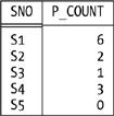
Note the tuple for supplier S5 in particular; the PER specification indicates that the summarizing is to be done “per the projection of S on SNO,” which means it produces a result with five tuples (one for each tuple in that projection). By contrast, the following SQL expression (which might be thought to be equivalent to the Tutorial D formulation):
  SELECT SP.SNO, COUNT(*) AS P_COUNT
  FROM   SP
  GROUP  BY SP.SNO
produces a result containing tuples for suppliers S1, S2, S3, and S4 only. The reason is, of course, that it extracts supplier numbers from SP, and supplier S5 doesn’t appear in SP at all. An SQL expression that is equivalent to the Tutorial D formulation is:
  SELECT S.SNO, TEMP.P_COUNT
  FROM   S, LATERAL ( SELECT COUNT(*) AS P_COUNT
            FROM   SP
            WHERE  SP.SNO = S.SNO ) AS TEMP
As I’ve already pointed out, however, not all SQL products support this kind of expression.
Note
The standard requires the keyword LATERAL here because the subquery refers “laterally” to another element in the same FROM clause.
Here now is the definition. Let r and s be relations such that s is of the same type as some projection of r, and let the attributes of s be A1, A2, . . ., An. Then the summarization:
SUMMARIZE r PER ( s ) ADD ( summary AS X )
is a relation with (a) heading equal to the heading of s extended with attribute X, and (b) body consisting of all tuples t such that t is a tuple of s extended with a value for attribute X. That X value is computed by evaluating summary over all tuples of r that have the same value for attributes A1, A2, . . . , An as tuple t does. Relation s must not have an attribute called X, and summary must not refer to X. Observe that the result has cardinality equal to that of s and degree equal to that of s plus one. The type of X in that result is the type of summary.
What “summaries” are supported? Well, the set is open-ended but certainly includes the usual COUNT, SUM, AVG, MAX, and MIN. Here’s an example involving MAX and MIN:
  SUMMARIZE SP PER ( SP { SNO } ) ADD ( MAX ( QTY ) AS MAXQ ,
                                        MIN ( QTY ) AS MINQ )
This example illustrates two further points:
It’s possible to perform “multiple summarizations” within a single SUMMARIZE. (I didn’t mention the point earlier, but analogous remarks apply to RENAME and EXTEND as well.)
The PER operand in this example isn’t just “of the same type as” some projection of the relation to be summarized, it actually is such a projection. In such cases the expression can be simplified slightly, as here:
  SUMMARIZE SP BY { SNO } ADD ( MAX ( QTY ) AS MAXQ ,
                                MIN ( QTY ) AS MINQ )
Other legal “summaries” include COUNTD, SUMD, and AVGD (where “D” stands for “distinct” and means “eliminate redundant duplicate values before summarizing”); AND, OR, and XOR (for attributes of type BOOLEAN); INTERSECT, UNION, and D_UNION (for relation-valued attributes); and so on.
By the way, COUNT and the rest here are not aggregate operators, though most of them do have the same names as aggregate operators (SQL confuses these two notions, with unfortunate results). An aggregate operator invocation is a scalar expression, and it returns a scalar value.[*] Here’s an example:
  VAR N INTEGER ;

  N := COUNT ( S WHERE CITY = 'London' ) ;
Summaries, by contrast, are merely operands to SUMMARIZE invocations; they have no meaning outside that context, and in fact can’t be used outside that context.
Here’s one more SUMMARIZE example (“How many suppliers are there in London?”):
SUMMARIZE ( S WHERE CITY = 'London' ) ADD ( COUNT () AS N )
Again, this example illustrates two points:
This SUMMARIZE has no PER specification. By default, therefore, the summarizing is done per TABLE_DEE— that is, the expression shown is shorthand for:
  SUMMARIZE ( S WHERE CITY = 'London' )
            PER ( TABLE_DEE ) ADD ( COUNT () AS N )
I remind you again that TABLE_DEE is the relation that has no attributes and one tuple (and is thus certainly of the same type as “some projection of” every possible relation!—namely, the projection of the relation in question on the empty set of attributes). The output from this SUMMARIZE therefore has one attribute and one tuple, and given our usual sample data values it looks like this:[*]
I said a moment ago that aggregate operator invocations and summaries were different things, and you might be wondering what the difference is between the SUMMARIZE example under discussion and the COUNT operator invocation we saw a few paragraphs back:
COUNT ( S WHERE CITY = 'London' )
The overriding difference is, of course, that SUMMARIZE returns a relation and aggregate operators return a scalar. For further discussion, see Exercise 5-11 at the end of this chapter.
Group and Ungroup
Recall from Chapter 2 that relations with relation-valued attributes (RVAs for short) are legal. Figure 5-1 shows relations R1 and R4 from Figures 2-1and 2-2 in that chapter; R4 has an RVA and R1 doesn’t, but the two relations clearly convey the same information.

Of course, we need a way to map between relations without RVAs and relations with them, and that’s the purpose of the GROUP and UNGROUP operators. I don’t want to go into a lot of detail on those operators here; let me just say that, given relations R1 and R4 as shown in Figure 5-1, respectively, the expression:
R1 GROUP ( { PNO } AS PNO_REL )
will produce R4, and the expression:
R4 UNGROUP ( PNO_REL )
will produce R1. SQL has no direct counterpart to these operators.
By the way: if R4 includes exactly one tuple for supplier number S x, say, and if the PNO_REL value in that tuple is empty, then the result of the foregoing UNGROUP will contain no tuple at all for supplier number S x. For further details, I refer you to my book An Introduction to Database Systems, Eighth Edition (Addison-Wesley, 2004) or the book Databases, Types, and the Relational Model: The Third Manifesto, Third Edition (Addison-Wesley, 2006), by Hugh Darwen and myself.
And by the way again: you might be wondering what operations on relations with RVAs look like. Well, operations on any relation, when they refer to some attribute A of that relation of type T, say, typically involve what we might call “suboperations” on values of that attribute A that are, precisely, operations that have been defined in connection with that type T. So if T is a relation type, those “suboperations” are operations that have been defined in connection with relation types—which is to say, they’re essentially the relational operations (join and the rest) described in the present chapter! See Exercises 5-27 through 5-30 at the end of this chapter.
Expression Transformation
I’ve now covered all of the algebraic operators I want to discuss in any detail, but there are some related topics that merit attention in this chapter. The first is the possibility of transforming a given relational expression into another, logically equivalent expression. I mentioned this possibility in Chapter 3, in the section "Why Duplicate Tuples Are Prohibited,” where I explained that such transformations are one of the things the optimizer does; in fact, such transformations constitute one of the two great ideas at the heart of relational optimization (the other, beyond the scope of this book, is the use of “database statistics" to do what’s called cost-based optimizing ). In this section, I want to say a little more about the process of expression transformation (or query rewrite , as it’s sometimes called). I’ll start with a trivial example. Consider the following expression (the query is “Get suppliers who supply part P2, together with the corresponding quantities”):
( ( S JOIN SP ) WHERE PNO = PNO('P2') ) { ALL BUT PNO }
Suppose there are 100 suppliers and 1,000,000 shipments, of which 500 are for part P2. If the expression is simply evaluated by brute force, as it were, without any optimization at all, the sequence of events is:
Join S and SP: This step involves reading the 100 supplier tuples; reading the 1,000,000 shipment tuples 100 times each, once for each of the 100 suppliers; constructing an intermediate result consisting of 1,000,000 tuples; and writing those 1,000,000 tuples back out to the disk. (I’m assuming for simplicity that tuples are physically stored as such, and I’m also assuming I can take “number of tuple I/O’s” as a reasonable measure of performance. Neither of these assumptions is realistic, but this fact doesn’t materially affect my argument.)
Restrict the result of Step 1: This step involves reading 1,000,000 tuples but produces a result containing only 500 tuples, which I’ll assume can be kept in main memory.
Project the result of Step 2: This step involves no tuple I/O’s at all, so we can ignore it.
The following procedure is equivalent to the one just described, in the sense that it produces the same final result, but is obviously much more efficient:
Restrict SP to just the tuples for part P2: This step involves reading 1,000,000 shipment tuples but produces a result containing only 500 tuples, which can be kept in main memory.
Join S and the result of Step 1: This step involves reading 100 supplier tuples (once only, not once per P2 shipment, because all the P2 shipments are in memory). The result contains 500 tuples (still in main memory).
Project the result of Step 2: Again we can ignore this step.
The first of these two procedures involves a total of 102,000,100 tuple I/O’s, whereas the second involves only 1,000,100; thus, it’s clear that the second procedure is over 100 times faster than the first. It’s also clear that we’d like the implementation to use the second procedure rather than the first! If it does, then it is (in effect) transforming the original expression:
( S JOIN SP ) WHERE PNO = PNO('P2')
(I’m ignoring the final projection now, since it isn’t really relevant to the argument) into the expression:
S JOIN ( SP WHERE PNO = PNO('P2') )
These two expressions are logically equivalent, but they have very different performance characteristics, as we’ve seen. If the system is presented with the first expression, therefore, we’d like it to transform it into the second before evaluating it—and of course it can. The point is that the relational algebra, being a high-level formalism, is subject to various formal transformation laws; for example, there’s a law that says a join followed by a restriction can be transformed into a restriction followed by a join (I was using that particular law in the example). And a good optimizer will know those laws, and will apply them—because, of course, the performance of a query shouldn’t depend on the specific syntax used to express that query in the first place. (Of course, it’s an immediate consequence of the fact that not all of the algebraic operators are primitive that certain expressions can be transformed into others—for example, an expression involving intersect can be transformed into one involving join instead—but there’s much more to it than that, as we’ll quickly see.)
Now, there are many possible transformation laws, and this isn’t the place for an exhaustive discussion. All I want to do is highlight a few important cases and key points. First, the law mentioned in the previous paragraph is actually a special case of a more general law, called the distributive law. In general, the monadic operator f distributes over the dyadic operator g if f(g(a,b)) = g(f(a),f(b)) for all a and b. In ordinary arithmetic, for example, SQRT (square root) distributes over multiplication, because:
SQRT ( a * b ) = SQRT ( a ) * SQRT ( b)
for all a and b (take f as SQRT and g as “*”); thus, a numeric expression optimizer can always replace either of these expressions by the other when doing numeric expression transformation. As a counterexample, SQRT does not distribute over addition, because the square root of a+b is not equal to the sum of the square roots of a and b, in general.
In relational algebra, restrict distributes over intersect, union, and difference. It also distributes over join, provided the restriction condition consists at its most complex of the AND of two separate conditions, one for each of the two join operands. In the case of the example discussed above, this requirement was satisfied—in fact, the restriction condition was very simple and applied to just one of the operands—and so we were able to use the distributive law to replace the expression with a more efficient equivalent. The net effect was that we were able to “do the restriction early.” Doing restrictions early is almost always a good idea, because it serves to reduce the number of tuples to be scanned in the next operation in sequence, and probably reduces the number of tuples in the output from that operation too.
Here are some other specific cases of the distributive law, this time involving projection. First, project distributes over intersect and union, though not difference. Second, it also distributes over join, so long as all of the joining attributes are included in the projection. These laws can be used to “do projections early,” which again is usually a good idea, for reasons similar to those given earlier for restrictions.
Two more important general laws are the laws of commutativity and associativity:
The dyadic operator g is commutative if g(a,b) = g(b,a) for all a and b. In ordinary arithmetic, for example, addition and multiplication are commutative, but division and subtraction aren’t. In relational algebra, intersect, union, and join are all commutative,[*] but difference and division aren’t. So, for example, if a query involves a join of two relations r and s,the commutative law tells us it doesn’t matter which of r and s is taken as the “outer” relation and which the “inner.” The system is therefore free to choose (say) the smaller relation as the “outer” one in computing the join.
The dyadic operator g is associative if g(a,g(b,c)) = g(g(a,b),c) for all a, b, c. In arithmetic, addition and multiplication are associative, but subtraction and division aren’t. In relational algebra, intersect, union, and join are all associative, but difference and division aren’t. So, for example, if a query involves a join of three relations r, s, and u, the associative and commutative laws together tell us we can join the relations pairwise in any order we like. (They also tell us it’s legitimate to define an n-adic or prefix version of the operator, as Tutorial D does.) The system is thus free to decide which of the various possible sequences is most efficient.
Observe that all of these transformations can be performed without any regard for either actual data values or actual storage structures (indexes and the like) in the database as physically stored. In other words, such transformations represent optimizations that are virtually guaranteed to be good, regardless of what the database looks like physically.
Relational Comparisons
In Chapter 2, I mentioned the fact that the equality comparison operator “=” applies to every type. In particular, therefore, it applies to relation types; that is, given two relations r and s of the same relation type T, we must at least be able to test whether those two relations are equal. Other comparisons might be useful, too; for example, we might want to test whether r is a subset of s (meaning every tuple in r is also in s), or whether r is a proper subset of s (meaning every tuple in r is also in s, but s contains at least one tuple that isn’t in r).
Now, I must immediately explain that these operators aren’t relational operators as such—that is, they’re not part of the relational algebra—because their result is a truth value, not a relation. But it’s convenient to discuss them in this chapter, and I will. Here’s a simple example:
S { CITY } = P { CITY }
The left comparand is the projection of suppliers on CITY, the right comparand is the projection of parts on CITY, and the comparison returns TRUE if these two projections are equal, FALSE otherwise. In other words, the comparison (which is, of course, a boolean expression) means: “Is the set of supplier cities equal to the set of part cities?”
Here’s another example:
S { SNO } ⊃ SP { SNO }
Explanation: The symbol "⊃" here means “is a proper superset of.” The meaning of this comparison (considerably paraphrased) is: “Are there any suppliers who supply no parts at all?”
Other useful relational comparison operators include "⊇" (“is a superset of”), "⊆" (“is a subset of”), and "⊂" (“is a proper subset of”).
The obvious place where relational comparisons are useful is in connection with restrictions.[*] Let’s look at some examples. Consider first the query “Get suppliers who supply all parts.” Here’s a possible formulation:
  WITH ( SP RENAME ( SNO AS X ) ) AS R :
       S WHERE ( R WHERE X = SNO ) { PNO } = P { PNO }
Explanation: The expression WITH . . . AS R is effectively equivalent to an assignment that assigns the value of the expression SP RENAME (SNO AS X) to some temporary, system-generated relvar R; after that assignment, the value of R is a relation that’s identical to the current value of relvar SP, except that attribute SNO has been renamed as X.[†] (The purpose of introducing the names R and X is simply to avoid a naming conflict that would subsequently arise otherwise.) Then, for a given supplier S x,say, in relvar S, the expression:
( R WHERE X = SNO ) { PNO }
evaluates to a relation with one attribute (PNO), giving part numbers for all parts supplied by supplier S x. Note in particular that if supplier S x supplies no parts, that relation will contain no tuples. Finally, that degree-one relation is tested for equality with the relation that’s the projection of P on PNO. Clearly, that test will give TRUE if and only if the set of part numbers for parts supplied by S x is equal to the set of part numbers in relvar P. The overall result thus contains precisely those tuples from relvar S that represent suppliers who supply all of the parts mentioned in relvar P.
Of course, we can write the entire query as a single expression if we like:
S WHERE ( ( SP RENAME ( SNO AS X ) ) WHERE X = SNO ) { PNO } = P { PNO }
But using WITH to introduce names for the results of subexpressions often helps to simplify the job of formulating complicated queries. Here’s a definition: if rx is a relational expression that mentions some relvar R, then WITH ry AS R: rx, where ry is another relational expression, is also a relational expression. Of course, rx might be a WITH expression, too, like this:
WITH ry AS R1 : WITH rz AS R2 : rx
This latter expression can be abbreviated to just:
WITH ry AS R1, rz AS R2 : rx
We’ll see plenty of examples of this abbreviated form later.
By the way, the foregoing example (“Get suppliers who supply all parts”) is very similar to one that’s often used to illustrate the use of the relational divide operator. To be specific, the expression:
SP { SNO, PNO } DIVIDEBY P { PNO }
(which I gave as an example of divide in the earlier section "The Original Operators“) is often characterized as a relational formulation of the query “Get supplier numbers for suppliers who supply all parts.” But it isn’t! Rather, it is a relational formulation of the query “Get supplier numbers for suppliers who supply at least one part and in fact supply all parts.” (If you’re wondering what the logical difference is here, see Exercise 5-25 at the end of this chapter.) In my opinion, the formulation involving a relational comparison is not only easier to understand than the divide formulation—it also has the advantage of being correct.
Here’s another example. The query is: “Get pairs of supplier numbers, S x and S y say, such that S x and S y supply exactly the same set of parts each.” This query is very difficult without relational comparisons! Here it is:
  WITH ( SP RENAME ( SNO AS SX ) ) { SX, PNO } AS R1 ,
     ( SP RENAME ( SNO AS SY ) ) { SY, PNO } AS R2 ,
     R1 { SX } AS R3 ,
     R2 { SY } AS R4 ,
     ( R1 JOIN R4 ) AS R5 ,
     ( R2 JOIN R3 ) AS R6 ,
     ( R1 JOIN R2 ) AS R7 ,
     ( R3 JOIN R4 ) AS R8 ,
     SP { PNO } AS R9 ,
     ( R8 JOIN R9 ) AS R10 ,
     ( R10 MINUS R7 ) AS R11 ,
     ( R6 JOIN R11 ) AS R12 ,
     ( R5 JOIN R11 ) AS R13 ,
     R12 { SX, SY } AS R14 ,
     R13 { SX, SY } AS R15 ,
     ( R14 UNION R15 ) AS R16 ,
     R7 { SX, SY } AS R17 :
  R17 MINUS R16
But with relational comparisons it’s fairly straightforward:
  WITH ( S RENAME ( SNO AS SX ) ) { SX } AS RX ,
     ( S RENAME ( SNO AS SY ) ) { SY } AS RY :
  ( RX JOIN RY ) WHERE ( SP WHERE SNO = SX ) { PNO } =
             ( SP WHERE SNO = SY ) { PNO }
As an aside, I remark that appending “AND SX < SY” to the WHERE clause here would produce a slightly tidier result; to be specific, it would (a) eliminate pairs of the form (S x,Sx) and (b) ensure that the pairs (Sx,Sy) and (Sy,Sx) don’t both appear.
One particular comparison that’s often needed in practice is an “=” comparison between a given relation r and an empty relation of the same type—in other words, a test to see whether r is empty. So let me introduce the following shorthand:
IS_EMPTY ( rx )
This expression is defined to return TRUE if the relation r denoted by the relational expression rx is empty and FALSE otherwise. I’ll be relying heavily on this construct in the next chapter.
Another common requirement is to be able to test whether a given tuple t appears in a given relation r:
  t
            ∊
            rx
This expression is defined to be shorthand for the relational comparison:
  RELATION { t } ⊆
            rx
The left operand here is a relation selector invocation, and it returns a relation containing just the specified tuple t. The comparison thus returns TRUE if t appears in the relation r denoted by the relational expression rx and FALSE otherwise (”∊" is the set membership operator; the expression t ∊ r can be read as "t[appears] in r“). In fact, as you’ve probably realized, the "∊" operator is essentially SQL’s IN operator—except that the left operand of SQL’s IN is usually a scalar, not a row, which means there’s some kind of coercion going on. Be that as it may, SQL certainly doesn’t support any relational comparisons apart from this rather special one. (Well, it does support NOT IN; so does Tutorial D, in the form of "∉“.)
More on Relational Assignment
The assignment operator “:=” resembles the equality comparison operator “=” in that it applies to every type, and relation types are no exception. Relational assignment in particular resembles “=” and the other comparison operators from the previous section in another respect as well: it isn’t part of the relational algebra. Why not? Because its target must be, very specifically, a relvar, not a relation (relvars aren’t part of the relational algebra either—there’s no notion of updating in the relational algebra as such, and “variable” means “updatable”). Nevertheless, I want to say a little more about relational assignment in this chapter; to be specific, I want to examine the INSERT, DELETE, and UPDATE shorthands a little more closely. As you know, these operators are just shorthand for certain relational assignments—but now I’m in a position to explain just what the “longhand” versions look like, in terms of appropriate algebraic operators. I’ll do this by showing some simple examples.
First, relational assignment in general looks like this:
R := rx
R here is a relvar and rx is a relational expression of the same type as R. The effect is to assign the relation r that’s denoted by the expression rx to the relvar R (and I remind you from the exercises in Chapter 2 that after the assignment, the boolean expression R = r is required to evaluate to TRUE: The Assignment Principle). Here’s a simple example:
  S := RELATION { TUPLE { SNO SNO('S1'), SNAME NAME('Smith'),
                                  STATUS 20, CITY 'London' } ,
                  TUPLE { SNO SNO('S2'), SNAME NAME('Jones'),
                                  STATUS 10, CITY 'Paris'  } ,
                  TUPLE { SNO SNO('S3'), SNAME NAME('Blake'),
                                  STATUS 30, CITY 'Paris'  } ,
                  TUPLE { SNO SNO('S4'), SNAME NAME('Clark'),
                                  STATUS 20, CITY 'London' } ,
                  TUPLE { SNO SNO('S5'), SNAME NAME('Adams'),
                                  STATUS 30, CITY 'Athens' } } ;
(As we saw in Chapter 3, the expression on the right here is another relation selector invocation; in fact, it’s a relation literal.)
Now I can turn to INSERT, DELETE, and UPDATE. Let relvar PQ be defined as follows:
VAR PQ BASE RELATION { PNO PNO, QTY QTY } KEY { PNO } ;
Here’s a possible INSERT on this relvar:
  INSERT PQ ( SUMMARIZE SP PER ( P { PNO } )
              ADD ( SUM ( QTY ) AS QTY ) ) ;
And here’s the “longhand” assignment equivalent:
  PQ := PQ UNION ( SUMMARIZE SP PER ( P { PNO } )
                 ADD ( SUM ( QTY ) AS QTY ) ) ;
In other words, the INSERT works by forming the union, pq say, of the old value of relvar PQ and the relation denoted by the SUMMARIZE invocation, and then assigning that relation pq to relvar PQ. (By the way, I’m assuming here that it’s not an error to insert a tuple that already exists in the target. If it is, that UNION in the expansion should be replaced by D_UNION.)
Next, a DELETE example:
DELETE S WHERE CITY = 'Athens' ;
Longhand equivalent:
S := S WHERE NOT ( CITY = 'Athens' ) ;
Finally, an UPDATE example:
  UPDATE P WHERE CITY = 'London'
       ( WEIGHT := 2 * WEIGHT , CITY := 'Oslo' ) ;
Longhand equivalent:
  P := WITH ( P WHERE CITY = 'London' ) AS R1 ,
            ( EXTEND R1 ADD ( 2 * WEIGHT AS NEW_WEIGHT,
                             'Oslo' AS NEW_CITY ) ) AS R2 ,
            R2 { ALL BUT WEIGHT, CITY } AS R3,
            R3 RENAME { NEW_WEIGHT AS WEIGHT, NEW_CITY AS CITY } AS R4,
            P MINUS R1 AS R5 :
            R5 UNION R4;
This one needs a little more explanation. First, R1 is the set of tuples to be updated (loosely speaking—see the section Chapter 4). Next, we extend each tuple in R1 with the applicable new WEIGHT and CITY values; that’s R2. Then we throw away the old WEIGHT and CITY values (that’s R3). Finally, we rename NEW_WEIGHT and NEW_CITY as WEIGHT and CITY, respectively (that’s R4); then we identify the set of tuples not to be updated (that’s R5), and assign the union of R5 and R4 to relvar P. Notice the use of the “multiple” forms of EXTEND and RENAME in this example.
The ORDER BY Operator
The last topic I want to address in this chapter is ORDER BY. ORDER BY is yet another operator that’s not part of the relational algebra; as I pointed out in Chapter 1, in fact, it isn’t a relational operator at all, because it produces a result that isn’t a relation (it does take a relation as input, but it produces something else—namely, a sequence of tuples— as output). Of course, I’m not saying ORDER BY isn’t useful; however, I am saying it can’t legally or sensibly appear in a relational expression.[*] By definition, therefore, the following expressions, though legal, aren’t relational expressions as such:
  S MATCHING SP        | SELECT DISTINCT S.*
    ORDER ( ASC SNO )  | FROM   S, SP
                       | WHERE  S.SNO = SP.SNO
                       | ORDER  BY S.SNO ASC
That said, I’d like to point out that for a couple of reasons ORDER BY (just ORDER, in Tutorial D) is actually a rather strange operator. First, it effectively works by sorting tuples into some specified sequence—and yet “<” and “>” aren’t defined for tuples (see Exercise 3-11 in Chapter 3). Second, it’s not a function. All of the operators of the relational algebra—in fact, all read-only operators, in the usual sense of that term—are functions, meaning there’s always just one possible output for any given input. By contrast, ORDER BY can produce several different outputs from the same input. As an illustration of this point, consider the effect of the operation ORDER BY CITY on our usual suppliers relation. Clearly, this operation can return any of four distinct results, corresponding to the following sequences (I’ll show just the supplier numbers, for simplicity):
  S5, S1, S4, S2, S3

  S5, S4, S1, S2, S3

  S5, S1, S4, S3, S2

  S5, S4, S1, S3, S2
A note on SQL: It would be remiss of me not to mention in passing that most of the algebraic operators have analogs in SQL that also aren’t functions. This state of affairs is due to the fact that, as indicated in the exercises in Chapter 2, SQL allows the comparison v1 = v2 to evaluate to TRUE even if v1 and v2 are distinct. For example, consider the character strings ‘Paris’ and ‘Paris ', respectively (note the trailing space in the latter); these values are clearly distinct, and yet SQL sometimes regards them as equal. As a consequence, certain queries give what the standard calls “possibly nondeterministic results.” Here’s a simple example:
SELECT DISTINCT S.CITY FROM S
If one supplier has CITY value ‘Paris’ and Paris ‘another ', then the result will include either or both of ‘Paris’ and ‘Paris ', but which result we get might be undefined. We could even legitimately get one result on one day and another on another, even if the database hasn’t changed at all in the interim. You might like to meditate on some of the implications of this state of affairs.
Summary
Almost inevitably, this has been the longest chapter in the book. Even so, I haven’t covered “all known” algebraic operators, nor have I explained every last detail of the ones I did cover; but I hope I have covered enough to give you a good sense of what the algebra is all about. To review briefly, here’s a list of the operators I did discuss: rename, restrict, project (including the ALL BUT form), join, semijoin (MATCHING), intersection, union, disjoint union (D_UNION), difference, semidifference (NOT MATCHING), product, divide, theta-join (including equijoin), extend, summarize, group, and ungroup. I also discussed certain nonalgebraic operators: relational comparisons, INSERT, DELETE, and UPDATE (and relational assignment), and ORDER BY. Other topics I covered include:
Closure: I explained the need for a set of relation type inference rules, so that we always know the type of the result of any given relational expression.
Primitive operators: I showed that many of the operators are in fact shorthand for certain combinations of others. In particular, intersect and product are special cases of join, and difference is a special case of semidifference.
Join: I also showed that—thanks to the fact that join is both commutative and associative—it was possible to define an n-adic or prefix version of the operator (where n is any integer greater than or equal to zero). The join of no relations at all is TABLE_DEE.
SQL expressions: I gave a conceptual algorithm for evaluating SQL SELECT - FROM - WHERE expressions. I also suggested that the SELECT - FROM - WHERE template is sometimes too rigid.
Summaries versus aggregate operators: I stressed the point (without getting into too much detail) that these are logically distinct constructs.
Expression transformation: I briefly explained the distributive, commutative, and associative laws and described their role in optimization (“query rewrite”).
WITH: I discussed the use of WITH in simplifying expression formulation by allowing names to be introduced for the results of subexpressions.
Exercises
Exercise 5-1.
From a relational perspective, what’s wrong (if anything) with the following SQL expressions?
  a. SELECT * FROM S, SP
  b. SELECT S.SNO, S.CITY FROM S
  c. SELECT SP.SNO, SP.PNO, 2 * SP.QTY FROM SP
  d. SELECT P.PNO FROM P
  e. SELECT S.SNO FROM S, SP
  f. SELECT S.SNO FROM S ORDER BY S.CITY DESC
Exercise 5-2.
Closure is important in the relational model for the same kind of reason that numeric closure is important in ordinary arithmetic. In arithmetic, however, there’s one situation where the closure property breaks down, in a sense—namely, division by zero. Is there any analogous situation in the relational algebra?
Exercise 5-3.
Given the usual suppliers-and-parts database, what’s the value of the expression JOIN{S,SP,P}? What’s the corresponding predicate? Warning: There’s a trap here; in fact, some might even argue that the trap is such that it makes join (as I’ve defined it in the body of this chapter) a rather dangerous operation. What do you think of that argument?
Exercise 5-4.
Why do you think the project operator is so called?
Exercise 5-5.
Given our usual sample values for the suppliers-and-parts database, what values do the following expressions denote? In each case, give an informal interpretation of the expression in natural language.
  a. S SEMIJOIN ( SP WHERE PNO = PNO('P2') )
  b. P NOT MATCHING ( SP WHERE SNO = SNO('S2') )
  c. S { CITY } MINUS P { CITY }
  d. ( S { SNO, CITY } JOIN P { PNO, CITY } ) { ALL BUT CITY }
  e. JOIN { ( S RENAME ( CITY AS SC ) ) { SC } ,
        ( P RENAME ( CITY AS PC ) ) { PC } }
Exercise 5-6.
Union, intersection, product, and join are all both commutative and associative. Verify these claims. Also verify that semijoin is associative but not commutative.
Exercise 5-7.
In what circumstances (if any) are r SEMIJOIN s and s SEMIJOIN r equivalent?
Exercise 5-8.
Which of the algebraic operators (if any) have a definition that doesn’t rely on tuple equality?
Exercise 5-9.
The SQL FROM clause FROM t1, t2, . . . , tn (where each ti is an expression denoting a table) returns the cartesian product of its arguments. But what if n = 1? What’s the cartesian product of just one table? And by the way, what’s the product of t1 and t2 if t1 and t2 both contain duplicate rows?
Exercise 5-10.
Show that rename isn’t primitive.
Exercise 5-11.
Distinguish between a “summary” and an aggregate operator. What do the SQL analogs of these constructs look like?
Exercise 5-12.
Give an expression involving EXTEND instead of SUMMARIZE that’s logically equivalent to the following:
SUMMARIZE SP PER ( S { SNO } ) ADD ( COUNT () AS NP )
Exercise 5-13.
Given our usual sample values for the suppliers-and-parts database, what values do the following expressions denote? In each case, give an informal interpretation of the expression in natural language.
  a. EXTEND S ADD ( 'Supplier' AS TAG )
  b. EXTEND ( P JOIN SP ) ADD ( WEIGHT * QTY AS SHIPWT )
  c. EXTEND P ADD ( WEIGHT * 454 AS GMWT, WEIGHT * 16 AS OZWT )
  d. EXTEND S
      ADD ( COUNT ( ( SP RENAME ( SNO AS X ) ) WHERE X = SNO )
        AS NP )
  e. SUMMARIZE S BY { CITY } ADD ( AVG ( STATUS ) AS AVG_STATUS )
Exercise 5-14.
Which of the following expressions are equivalent?
  a. SUMMARIZE r PER ( r { } ) ADD ( COUNT () AS CT )
  b. SUMMARIZE r ADD ( COUNT () AS CT )
  c. SUMMARIZE r BY { } ADD ( COUNT () AS CT )
  d. EXTEND TABLE_DEE ADD ( COUNT ( r ) AS CT )
Exercise 5-15.
Simplifying just slightly, an aggregate operator invocation in Tutorial D takes the form:
<agg op name> ( <relation exp> [, <attribute name> ] )
If the <agg op name> is COUNT, the <attribute name> is irrelevant and must be omitted; otherwise, it can be omitted if and only if the <relation exp> denotes a relation of degree one, in which case the sole attribute of the result of that <relation exp> is assumed by default. Here are a couple of examples:
  SUM ( SP WHERE SNO = SNO('S1'), QTY )
  SUM ( ( SP WHERE SNO = SNO('S1') ) { QTY } )
Note the difference between these two expressions: the first gives the total of all shipment quantities for supplier S1, and the second gives the total of all distinct shipment quantities for supplier S1. How does the scheme just outlined differ from its SQL counterpart?
Exercise 5-16.
In Tutorial D, if the argument to an aggregate operator invocation happens to be an empty set, COUNT returns zero and so does SUM; MAX and MIN return, respectively, the lowest and the highest value of the applicable type; AND and OR return TRUE and FALSE, respectively; and AVG raises an exception (I ignore Tutorial D’s other aggregate operators here deliberately). What does SQL do in these circumstances and why?
Exercise 5-17.
Let relation R4 from Figure 5-1 denote the current value of some relvar R. If R4 has the meaning described in Chapter 2, give the predicate for that relvar R.
Exercise 5-18.
Let r be the relation denoted by the following expression:
SP GROUP ( { } AS X )
What does r look like, given our usual sample value for SP? Also, what does the following expression yield?
r UNGROUP ( X )
Exercise 5-19.
Without using the IS_EMPTY shorthand, write a Tutorial D expression that returns TRUE if the current value of the parts relvar P is empty and FALSE otherwise. Also show an SQL analog of that expression.
Exercise 5-20.
Write Tutorial D and/or SQL expressions for the following queries on the suppliers-and-parts database:
Get all shipments.
Get supplier numbers for suppliers who supply part P1.
Get suppliers with status in the range 15 to 25 inclusive.
Get part numbers for parts supplied by a supplier in London.
Get part numbers for parts not supplied by any supplier in London.
Get city names for cities in which at least two suppliers are located.
Get all pairs of part numbers such that some supplier supplies both of the indicated parts.
Get the total number of parts supplied by supplier S1.
Get supplier numbers for suppliers with a status lower than that of supplier S1.
Get supplier numbers for suppliers whose city is first in the alphabetic list of such cities.
Get part numbers for parts supplied by all suppliers in London.
Get supplier-number/part-number pairs such that the indicated supplier does not supply the indicated part.
Get suppliers who supply at least all parts supplied by supplier S2.
Get supplier numbers for suppliers who supply at least all parts supplied by at least one supplier who supplies at least one London part.
Exercise 5-21.
Prove the following statements (making them more precise, where necessary):
A sequence of restrictions against a given relation can be transformed into a single restriction.
A sequence of projections against a given relation can be transformed into a single projection.
A restriction of a projection can be transformed into a projection of a restriction.
Exercise 5-22.
Union is said to be idempotent, because r UNION r is identically equal to r for all r. (Is this true in SQL?) As you might expect, idempotence can be useful in expression transformation. Which other relational operators (if any) are idempotent?
Exercise 5-24.
The following boolean expression:
x > y AND y > 3
(which might be part of a query) is clearly equivalent to—and can therefore be transformed into—the following:
x > y AND y > 3 AND x > 3
The equivalence is based on the fact that the comparison operator “>” is transitive. The transformation is worth making if x and y are from different relations, because it enables the system to perform an additional restriction (using x > 3) before doing the greater-than join implied by x > y. As we saw in the body of the chapter, doing restrictions early is generally a good idea; having the system infer additional “early” restrictions, as here, is also a good idea. Do you know of any commercial products that actually perform this kind of optimization?
Exercise 5-25.
Consider the following expressions:
  a. WITH ( P WHERE COLOR = 'Purple' ) AS PP ,
      ( SP RENAME ( SNO AS X ) ) AS T :
     S WHERE ( T WHERE X = SNO ) { PNO } ⊇ PP { PNO }

  b. WITH ( P WHERE COLOR = 'Purple' ) AS PP :
     S JOIN ( SP { SNO, PNO } DIVIDEBY PP { PNO } )
These are both attempts at formulating the query “Get suppliers who supply every purple part.” Given our usual sample data values, show the result returned in each case. Which result (and which formulation), if either, do you regard as correct? Justify your answer.
Exercise 5-26.
Consider the restriction r WHERE bx. In the body of the chapter, I said that every attribute mentioned in the restriction condition bx must be an attribute of r, but I also mentioned that bx was subject to certain further limitations. One of those limitations[*] is that, strictly speaking, bx is supposed to consist of just a single term of the form x Op y,where each of x and y is either an attribute of r or a literal and Op is a comparison operator that makes sense for x and y. But a real language will allow WHERE clauses to contain boolean expressions of arbitrary complexity, just as long as the only “free variables” (see Appendix A) in that expression are attributes of r. Show that it’s legitimate to extend the definition of restrict in such ways—that is, show that such extensions are really just shorthand for something we already know is legitimate.
Exercise 5-27.
Here are two simple expressions involving relation R4 from Figure 5-1 in the body of the chapter. What queries do they represent?
  ( R4 WHERE TUPLE { PNO PNO('P2') } ∊PNO_REL ) { SNO }

  ( ( R4 WHERE SNO = SNO('S2') ) UNGROUP ( PNO_REL ) ) { PNO }
Exercise 5-28.
Given our usual sample values for the suppliers-and-parts database, what does the following expression denote?
  EXTEND S
     ADD ( ( ( SP RENAME ( SNO AS X ) ) WHERE X = SNO ) { PNO }
      AS PNO_REL )
Exercise 5-29.
Let the relation returned by the expression in the previous exercise be kept as a relvar called SSP. What do the following updates do?
  INSERT SSP RELATION
    { TUPLE { SNO SNO('S6'),
        PNO_REL RELATION { TUPLE { PNO PNO('P5') } } } } ;

  UPDATE SSP WHERE SNO = SNO('S2')
    ( INSERT PNO_REL RELATION { TUPLE { PNO PNO('P5') } } ) ;
Exercise 5-30.
Using relvar SSP from the previous exercise, write expressions for the following queries:
Get pairs of supplier numbers for suppliers who supply exactly the same set of parts.
Get pairs of part numbers for parts supplied by exactly the same set of supliers.
[*] Not in SQL, though! For example, if R and S are SQL table names, we typically can’t write things like R UNION S; instead, we have to write something like SELECT R.* FROM R UNION SELECT S.* FROM S.
[*] I once wrote a paper on this topic called “Fifty Ways to Quote Your Query” (www.dbpd.com, July 1998), in which I showed that even a query as simple as “Get names of suppliers who supply part P2” can be expressed in well over 50 different ways in SQL.
[*] The boolean expression is subject to certain other limitations as well. See Exercise 5-6 at the end of the chapter.
[*] I’ll discuss other kinds of joins in the next section.
[*] Tutorial D doesn’t directly support “the original and simplest” divide, and this is thus not valid Tutorial D syntax.
[*] So long as s isn’t empty. What happens if it is?
[*] If theta had been “=” instead of “≠”, Step 2 would have been: Restrict the cartesian product by retaining just the rows in which the two city values are equal—in which case we would now have formed what’s called the equijoin of suppliers and parts on cities. In other words, an equijoin is a theta-join for which theta is “=”. Exercise: What’s the difference between an equijoin and a natural join?
[*] It’s true—thanks to, among other things, the ability to nest subqueries in the FROM clause—that the operands to that cartesian product aren’t limited to being named tables (base tables or views), but the FROM clause as such still basically means cartesian product.
[*] Nonscalar aggregate operators can be defined too, but they’re beyond the scope of this book.
[*] The fact that the picture involves no double underlining is not a mistake. See Exercise 4-28 in Chapter 4.
[*] Strictly speaking, join is not commutative in SQL, because SQL attaches significance to the left-to-right ordering of columns, and r JOIN s and s JOIN r thus differ in their result column orderings.
[*] But see Exercise 5-26 at the end of the chapter.
[†] SQL supports WITH too, though it writes the operands the other way around: WITH name AS expression.
[*] In particular, therefore, it can’t appear in a view definition—despite the fact that at least one well-known product allows it to!
[*] Another is that bx mustn’t involve any quantifiers, nor must it be equivalent to an expression that does (see Appendix A).