
17
COMMUNICATIONS THROUGH BANDLIMITED TIME‐INVARIANT LINEAR CHANNELS
17.1 INTRODUCTION
In this chapter, the analysis and simulation of bandlimited time‐invariant linear communication channels is discussed. The channel is viewed in broad terms and may include the transmitter and receiver filtering as well as the transmission medium. The linear time‐invariant channel is frequently encountered in practice and is relatively easy to analyze and simulate. Since these channels are often related to classical filter theory, the analysis and application of linear filters draw on the abundance of time‐tested work related to filter theory and design.
In communication systems, the channel distortion manifests itself in two distinct ways: the transmitted waveform is distorted in such a way that the received symbol energy within the symbol interval is reduced leading to a loss in signal‐to‐noise ratio (SNR); the channel distortion results in dispersion of the symbol energy into adjacent symbols resulting in noise‐like terms referred to as intersymbol interference (ISI). The channel distortion results from the amplitude and phase responses of the channel that becomes increasingly severe as the waveform bandwidth approaches the channel bandwidth. The ISI results in the closing of the demodulator eye‐opening at the sampled matched filter output that reduces the probability of a correct decision. It also impacts the symbol timing and carrier phase tracking functions of the demodulator that often take advantage of distinct spectral properties of the modulated waveform.
Because the ISI under consideration results from a linear time‐invariant channel, it is deterministic with respect to a known symbol; however, it appears to be random because of the randomly modulated stream of contiguous symbols. ISI cancellation is embodied in the subject of equalization that is based upon this deterministic nature of the ISI. Although the statistical distribution characterizing the ISI is not generally known by the demodulator, estimates, based on the demodulated data,* are formed to cancel the ISI, thereby, improving the system’s performance [1].
In this chapter, the channels are characterized in the frequency domain in terms of amplitude and phase responses that can be arbitrarily specified. Typical channel characterizations include classical filters like the Butterworth and Chebyshev designs and dial‐up wireline channels [2, 3] with or without various degrees of conditioning, for example, C1 and C2 designated conditioning. The phase response can be specified independently of the amplitude response and transmissions through phase‐equalized channels demonstrate a marked improvement in performance. Although the analysis permits applying arbitrarily specified modulation functions, examples involving rectangular modulated waveforms applied to channels with quadratic and cubic phase responses are examined to demonstrate the effects of channel distortion. The analysis is based on the work of Sunde [4] and Urkowitz [5]; in that, the inphase and quadrature (I/Q) responses of the low‐pass equivalents of bandpass filters are developed. With digital signal processing, the lowpass filter is a computationally efficient way to perform bandpass filtering; however, in most applications, the lowpass or baseband filtered output is used directly for subsequent signal processing and matched filter detection. The analysis also highlights the use of complex notations, in which the I/Q components are the real and imaginary parts of complex functions referred to as pre‐envelopes [6].
In Section 17.2, some basic filter concepts are established to generate real carrier and baseband modulated outputs based on an arbitrary input signal. In Section 17.3, an input carrier modulated signal is filtered using a baseband filter with appropriate frequency heterodyning. Sections 17.4 and 17.5 characterize a rect(t/T) input signal and develops the output response for an arbitrarily specified filter. The filter is expressed in terms of the I/Q amplitude and phase impulse responses. The parameters of the signal and filter response functions are then conveniently normalized for computer evaluation. In Sections 17.6 and 17.7, the responses of an ideal rect(u/B)/B filter and a single‐pole bandpass filter are examined using the computer model. The chapter concludes with computer simulated examples relating the characteristics of the ISI to various channel phase and amplitude characteristics.
17.2 INPHASE AND QUADRATURE CHANNEL RESPONSE
In this section, generalized expressions for the bandpass channel impulse response are developed in terms of the I/Q responses of the equivalent lowpass filter. Expressing a bandlimited channel impulse response in this form provides considerable insight into the channel characteristics. Consider the time‐invariant linear channel having a transfer function or frequency response given by H(ω). Because only real impulse responses are of interest, the transfer function exhibits an even real part and odd imaginary part in frequency.2 The channel transfer function, expressed in terms of real and imaginary parts, is
and the impulse response is defined as the inverse Fourier transform, expressed as

Because only real impulse responses are of interest, the functions Hr(ω) and Hi(ω) must be, respectively, even and odd functions of frequency. Expressing H(ω) in terms of positive and negative frequency functions, (17.1) is rewritten as

where ωc is any convenient reference frequency for H(ω); usually ωc is chosen as the mid‐band or the arithmetic mean of the upper and lower channel cutoff frequencies. Defining the lowpass frequency as ![]() , the positive and negative frequency functions in (17.3) have equivalent lowpass functions centered at ±ωc as depicted in Figure 17.1.
, the positive and negative frequency functions in (17.3) have equivalent lowpass functions centered at ±ωc as depicted in Figure 17.1.

FIGURE 17.1 Channel filter characteristics.
Rewriting (17.2) in terms of the lowpass frequency ![]() with
with ![]() results in
results in

Equating the equivalent lowpass expressions for the real and imaginary parts Hr(u) and Hi(u) of (17.3) results in ![]() and
and ![]() . Upon using the even or odd symmetry property then either Hr(u) = 2Hc(u) or Hi(u) = 2Hs(u), so that (17.4) becomes
. Upon using the even or odd symmetry property then either Hr(u) = 2Hc(u) or Hi(u) = 2Hs(u), so that (17.4) becomes

where

and

The functions hc(t) and hs(t) are, respectively, the lowpass I/Q impulse responses of the bandpass channel filter H(ω). In general, Hc(u) and Hs(u) will not possess either even or odd symmetry; however, if even or odd symmetry does exist, then either hc(t) or hs(t) will be zero.
The magnitude and phase functions of the baseband filter output are computed, respectively, as
and
Using (17.8) and (17.9), the lowpass frequency response is expressed as
Substituting (17.10) into (17.5), the quadrature responses in (17.6) and (17.7) are evaluated as

and

The lowpass equivalent filter, characterized in this section, is used in Section 17.3 to describe the lowpass filtering of an arbitrary carrier modulated input signal.
17.3 INPHASE AND QUADRATURE CHANNEL RESPONSE TO ARBITRARY SIGNAL
In Section 17.2, the impulse response of a bandpass channel, centered at an angular frequency of ωc, is expressed in terms of I/Q lowpass channel functions. In this section, the lowpass channel response is examined for an arbitrary real input signal in terms of the equivalent lowpass filter functions. Figure 17.2 shows the functional implementation with the channel’s lowpass impulse response functions, hc(t) and hs(t), developed in Section 17.2.

FIGURE 17.2 Lowpass filtering of carrier modulated signal.
The arbitrary carrier modulated input signal s(t) is expressed as
where ωs is the signal angular carrier frequency and sc(t) and ss(t) are the quadrature components that characterize the baseband modulation. The input carrier frequency is intentionally offset from the channel frequency so that the impact of the frequency error ![]() can be examined in the subsequent example applications.
can be examined in the subsequent example applications.
A completely analogous but considerably easier implementation to analyze and less prone to analysis errors is based on the analytic or complex signal representations shown in Figure 17.3. The input carrier frequency of ωs is offset from the channel filter’s center frequency by Δω and must be considered in evaluating the output of the lowpass filter, defined by the convolution integral


FIGURE 17.3 Analytic lowpass filtering of carrier modulated signal.
The integral in the second equality of (17.14) is defined as ![]() , such that,
, such that,

Using these relationships, the composite lowpass filter is described as shown in Figure 17.3.
The final up‐conversion to the output frequency ωo may represent an intermediate frequency (IF) of a linear heterodyning receiver. In this case, all of the intervening filtering of the linear receiver must be included in the lowpass filter function ![]() . If the lowpass channel filter includes the entire receiver and demodulator filtering prior to the baseband conversion in the demodulator, then no up‐conversion is necessary. However, the coherent demodulator Costas phaselock loop must remove the frequency error Δω. On the other hand, if the receiver expects the received signal frequency to be ωs, using the up‐conversion frequency ωs, instead of ωo − Δω, results in the receiver input frequency ωs + Δω, in which case, the frequency error must be removed by the coherent demodulator phaselock loop.
. If the lowpass channel filter includes the entire receiver and demodulator filtering prior to the baseband conversion in the demodulator, then no up‐conversion is necessary. However, the coherent demodulator Costas phaselock loop must remove the frequency error Δω. On the other hand, if the receiver expects the received signal frequency to be ωs, using the up‐conversion frequency ωs, instead of ωo − Δω, results in the receiver input frequency ωs + Δω, in which case, the frequency error must be removed by the coherent demodulator phaselock loop.
In the following evaluation of the filter output, the analytic functions ![]() and
and ![]() are defined as
are defined as
and
where the asterisk denotes the convolution of ![]() and
and ![]() that follows directly from (17.14) with
that follows directly from (17.14) with ![]() defined in (17.15).
defined in (17.15).
Therefore, expressing the analytic functions ![]() , and
, and ![]() in terms of their respective quadrature components, having the form
in terms of their respective quadrature components, having the form ![]() , the analytic lowpass filter output function,
, the analytic lowpass filter output function, ![]() , is evaluated using (17.14) and (17.15), and the result is expressed as
, is evaluated using (17.14) and (17.15), and the result is expressed as

The second and fourth terms in (17.18), that is, the terms involving sin(Δωλ), correspond, respectively, to the quadrature components of the third and first terms. For coherent demodulation, these terms are eliminated by the demodulator phaselock loop tracking prior to data detection. The quadrature components, ![]() and
and ![]() , correspond, respectively, to the real and imaginary parts of
, correspond, respectively, to the real and imaginary parts of ![]() and, upon substitution into (17.18), the complex lowpass filter output is expressed as
and, upon substitution into (17.18), the complex lowpass filter output is expressed as

The real part of (17.19) simplifies to
and, when the transmitted signal carrier frequency is equal to ωc with Δω = 0, (17.20) simplifies to

However, when the output is mixed to the carrier frequency ωo, as shown in Figure 17.3, the received signal is characterized as the real signal given by
where

and

17.3.1 Frequency Domain Characterization of Lowpass Filter Output
In this section, the lowpass channel filter response is described in terms of the frequency domain representation of the lowpass signal and the channel filter. The simulation processing discussed in Section 17.5 and the simulation results discussed in Sections 17.6 and 17.7 use the frequency response functions. In this description, the signal phase ϕ and the frequency error ∆ω are introduced to characterize the rect(t/T) modulated signal phase at the input to the channel filter. This signal phase and frequency error are used in Section 17.4 in describing the signal.
For the linear filtering operations being considered, the spectrum of the lowpass filter output (![]() ) is the product of the signal and channel filter spectrums, expressed as
) is the product of the signal and channel filter spectrums, expressed as
where the signal spectrum is based on the Fourier transform of ![]() expressed as
expressed as

Substituting (17.26) into (17.25) with the channel filter spectrum equal to ![]() , as developed in Section 17.2, results in the channel filter spectrum
, as developed in Section 17.2, results in the channel filter spectrum

The channel output is evaluated as the inverse Fourier transform of (17.27) and is expressed as
where

and

17.4 PULSE MODULATED CARRIER SIGNAL CHARACTERISTICS
In this section, a binary phase shift keying (BPSK) modulated carrier signal is characterized by the rect(t/T) modulation function with amplitude A volts, binary data dc = ±1, and angular carrier frequency ωs. An isolated symbol is expressed as

Because BPSK modulation is being considered, the quadrature data ds = 0, so the quadrature signal term ss(t) in (17.31) corresponds to the quadrature component of the inphase modulated symbol resulting from the signal phase error ϕ.
When the signal s(t) is mixed to baseband, using the channel carrier frequency, ωc, the resulting baseband symbol is expressed as

The spectrum of the baseband signal ![]() is evaluated using the Fourier transform and is expressed as
is evaluated using the Fourier transform and is expressed as

and is shown in Figure 17.4.

FIGURE 17.4 BPSK symbol baseband spectral characteristics (ϕ > 0).
Using this ideal, infinite bandwidth, form of the transmitted symbol does not detract from the generality of a performance simulation because the bandwidth limiting characteristics of a practical transmit filter can often be included as part of the underlying channel filter. However, without a transmit filter to contain the transmitted signal spectrum, the time–frequency product fsT would have to meet the condition fsT ≫ 1 in order to contain the signal spectrum fold‐over about the zero‐frequency axis.3
In Section 17.5, these relationships, describing the signal, are combined with those describing the channel to characterize the channel output response under a variety of conditions.
17.5 CHANNEL RESPONSE TO A PULSED MODULATED WAVEFORM
The channel response to the pulse modulated carrier signal described in Section 17.4 is characterized in this section. If the receiver filtering functions are included in the channel description along with the transmitter filtering functions, as mentioned in Section 17.1, then the response can be viewed as the input to the demodulator detection filter. If the demodulator matched filter response is also included in the channel description, then the response to the modulated waveform can be optimally sampled for subsequent data decision processing. The lowpass channel output is evaluated using (17.28), repeated here as
For the BPSK modulated signal described in Section 17.4, the quadrature components of (17.34) are evaluated using (17.29) and (17.30) with Ss(u) = 0. The resulting expressions are

and

These relationships are evaluated in Sections 17.6 and 17.7 to characterize the channel output for the pulse modulated symbol spectrum as described in Section 17.4. The amplitude and phase descriptions of the channel, as described by (17.8) and (17.9), respectively, are useful; in that, the magnitude and phase responses can be independently changed to examine the response under various channel conditions. When applied to the signal spectrum, the phase response can be altered to examine the effect of frequency errors and signal delays.
17.5.1 Normalized Channel Impulse Response
There are a number of advantages to normalize the channel response expressions for computer simulations. For example, the normalized expressions often apply to any system regardless of the carrier frequency or bandwidth.4 The use of very large or small numbers is avoided making input easier and less prone to errors, and the parameters are combined resulting in fewer parametric results required to characterize the system performance. For these reasons, the preceding relationships involving the channel response are evaluated in normalized form for subsequent computer programming and performance evaluation.
In this section, the channel impulse responses expressed by (17.5), (17.6), and (17.7) are normalized for computer simulation. The signal sampling rate must be selected to satisfy the Nyquist sampling criteria, so it is necessary to integrate the frequency over an adequate number of channel bandwidths relative to the center frequency. Although the baseband channel simulation is the primary interest, the simulation also characterizes the carrier modulated input and output signals which require satisfying the Nyquist bandpass sampling criterion. Defining the lowpass or one‐sided baseband channel bandwidth as B, the normalized frequency variable is defined as ![]() ; the normalized dependent variable is defined as Y = tB. With these normalizations the differential of u is
; the normalized dependent variable is defined as Y = tB. With these normalizations the differential of u is ![]() . The normalized parameters Fk and ρ are defined as Fk = fc/B and ρ = BT. Substituting these parameters into the impulse response expression given by (17.5) results in
. The normalized parameters Fk and ρ are defined as Fk = fc/B and ρ = BT. Substituting these parameters into the impulse response expression given by (17.5) results in
where

and

17.5.2 Normalized Symbol Pulse Response
The parameter normalization is the same as for the channel filter defined in Section 17.5.1; however, in this case, there are two additional normalizations to consider. The normalized signal delay is defined as Yd = τ/T and the normalized signal frequency shift is defined as Xd = (fs − fc)/B. The isolated symbol pulse is considered to have a positive amplitude with dc = 1. The parameter normalizations are summarized in Table 17.1.
TABLE 17.1 Normalized Parameter Definitions
| Parameter | Definition | Normalized Description |
| Y | t/T | Time |
| Yd | τ/T | Symbol delay |
| X | (f − fc)/B | Frequency, u/2πB |
| Xd | (fs − fc)/B | Signal frequency shift |
| dX | Δf/B | Differential frequency, Δu/2πB |
| Fk | fc/B | Channel frequency |
| fs/B | Signal frequency | |
| ϕ′(X) | — | Frequency‐dependent phase |
| ρ | BT | Channel‐to‐signal bandwidth |
For the pulsed carrier modulated signal, the channel responses in (17.34), (17.35), and (17.36) are expressed in normalized form as

where

and

with
Defining the lowpass frequency variable ![]() with respect to the signal frequency, the translation between the channel and signal frequencies is simply
with respect to the signal frequency, the translation between the channel and signal frequencies is simply ![]() or, in normalized form,
or, in normalized form, ![]() .
.
17.6 EXAMPLE PERFORMANCE SIMULATIONS
In this section, the channel output is examined under several conditions using computer simulations and the normalized parameters defined in Table 17.1. Figure 17.5 shows the various parameters relative to the signal and channel implementation. The signal delay τ results in a propagation phase of φ = −2πfsτ radians that is included in the signal phase ϕ. In the frequency domain, the delay is evident as a linear phase function with frequency. In these evaluations, the simulation program performs a numerical integration over a finite number of channel bandwidths covering the frequency range kB. Since the signal bandwidth is less than the channel bandwidth, the frequency sampling resolution of δf = 1/k1T is used. The total number of frequency samples is ![]() where ρ = BT is the number of signal bandwidths contained in the bandwidth of the filter. The sampling resolution and the total number of samples are chosen simply to provide for a high fidelity plot of the respective signal and filter spectrums and generally exceed the minimum sample rate required by the Nyquist criterion. If the carrier frequency is under sampled, because the time sample increment Δt is too large for the specified carrier frequency, the simulation outputs only the baseband responses gc(Y) and gs(Y).
where ρ = BT is the number of signal bandwidths contained in the bandwidth of the filter. The sampling resolution and the total number of samples are chosen simply to provide for a high fidelity plot of the respective signal and filter spectrums and generally exceed the minimum sample rate required by the Nyquist criterion. If the carrier frequency is under sampled, because the time sample increment Δt is too large for the specified carrier frequency, the simulation outputs only the baseband responses gc(Y) and gs(Y).

FIGURE 17.5 Signal and channel parameter descriptions.
17.7 EXAMPLE OF CHANNEL AMPLITUDE AND PHASE RESPONSES
In this section, several channel amplitude and phase functions are considered and example responses for the pulse modulated carrier input are examined. First, an ideal bandpass channel having constant amplitude and linear phase is considered, and the Gibbs phenomenon [7] is demonstrated in the computer simulation results. The Gaussian channel is then examined followed by a single‐pole bandpass filter representation of the channel. The single‐pole filter is representative of the antenna response for very‐low‐frequency (VLF) through high‐frequency (HF) systems, and the resulting ISI is characterized for various filter (antenna) bandwidths. The final simulation examines the amplitude and phase response of a dial‐up voice grade telephone circuit with and without delay equalization. In this case, several interesting characteristics of the ISI are examined. An example list of simulation conditions is provided in Table 17.2.
TABLE 17.2 Example Conditions for Channel Response
| Parameter | Value | Description |
| fc | 2.4 | kHz |
| B | 1.2 | kHz |
| Yd | 1.5 | Signal delay |
| fs | 2.4 | kHz |
| Rs | 0.15 | ksps |
| Fd | 0.075 | Constant delay |
| ϕ′(X) | — | Frequency‐dependent phasea |
| ϕc | 0.0 | Carrier phase (degrees) |
| Fd1 | 0.0 | Linear delay coefficienta |
| Fd2 | ±5.0 | Quadratic delay coefficienta |
aSee Sections 17.8.2 and 17.8.3.
17.7.1 Ideal Bandpass Channel
The ideal bandpass channel is examined to demonstrate the nature of channel distortion under ideal conditions. The ideal bandpass channel is characterized as having a constant amplitude over the entire bandwidth with zero response otherwise. The phase function of the ideal bandpass channel is linear and results in a constant signal delay. In terms of the lowpass frequency variable u = ω − ωc the amplitude and phase responses are expressed as
and
where ϕc is the channel phase shift at the channel frequency and the frequency dependent phase function, previously defined as ϕ′(u), is given by ![]() . The normalized expressions used in the simulation are
. The normalized expressions used in the simulation are

and
where Yd = τ/T is the normalized channel delay.
The response to a pulse modulated carrier is shown in Figure 17.6 for the conditions listed in Table 17.2. Figure 17.6a shows the channel and signal spectral characteristics, and Figure 17.6b and c shows the respective carrier and baseband responses. The oscillations in the responses about the pulse edges result from the Gibbs phenomenon and are caused by the finite number of terms in the Fourier expansion of the output resulting from the finite channel bandwidth. The normalized signal delay of 1.5 will normally center the response about Y = 1.5. However, the normalized channel delay of 0.075 associated with the slope of the phase functions results in the center of the response corresponding to Y = 1.575. The quadrature response in Figure 17.6c is zero because the channel is symmetrical with respect to the signal spectrum.

FIGURE 17.6 Response to ideal bandlimited channel.
17.7.2 Single‐Pole Channel Filter
Amplitude functions characterized as single‐pole filters are often useful in characterizing channels modeled as VLF antennas. The response for a single‐pole filter with a zero at the origin of the s‐plane is given by

where the poles are located at ![]() . By letting
. By letting ![]() , the positive frequency spectrum, expressed in terms of the lowpass frequency u = ω − ωc, is evaluated as
, the positive frequency spectrum, expressed in terms of the lowpass frequency u = ω − ωc, is evaluated as
where the frequency‐dependent phase is ![]() and the channel constant phase shift is
and the channel constant phase shift is ![]() . The 3 dB bandwidth is readily evaluated as B = α/2π and the resulting normalized form of the amplitude and phase responses are given by
. The 3 dB bandwidth is readily evaluated as B = α/2π and the resulting normalized form of the amplitude and phase responses are given by
and


The normalized channel delay is defined as the slope of the phase function at u = 0 and is evaluated as

Various responses to the single‐pole channel model are shown in Figure 17.7 for the conditions listed in Table 17.2 with the following exceptions: the channel phase ϕc is computed using (17.51), ϕ′(X) is computed using (17.52), and the channel bandwidth is B = 150 Hz so the BT product is unity. Figure 17.7a shows the channel and signal spectral characteristics, and Figure 17.7b and c show the carrier and baseband responses, respectively. Under ideal conditions, the channel responses are symmetrical about Y = 1.5 with the energy essentially confined to the interval |Y − 1.5| < 0.5. However, because of the channel amplitude and phase functions, the responses are asymmetrically distorted with considerable signal energy exceeding Y = 2. In the case of a continuous stream of information symbols this distortion or dispersion results in predominately postsymbol interference and degraded performance in the information recovery process because of the ISI. In Section 17.8.2 the channel characteristics resulting in predominately pre‐ and postsymbol interference are examined. As in the case of the ideal channel, the quadrature response in Figure 17.7c is zero because the channel is symmetrical with respect to the signal spectrum.

FIGURE 17.7 Response to single‐pole channel model (BT = 1).
The demodulator matched filter response can also be included in the channel characterization. In an additive white Gaussian noise (AWGN) environment, the frequency response of the matched filter is the amplitude scaled complex conjugate of the transmitted signal spectrum with an associated arbitrary delay. Considering the transmitted signal described in Section 17.4, the demodulator matched filer is characterized as
where K is an arbitrary scale factor and To is an arbitrary filter delay. Incorporating this matched filter response as part of the overall channel response, the demodulator baseband output for BT = 0.5 is shown in Figure 17.8. Aside from these changes, the channel conditions used in Figure 17.7 are identical. The optimally sampled matched filter output in Figure 17.8 corresponds to Y = 1.715. In a sequence of contiguous received symbols, the demodulator symbol synchronization processing must sample the matched filter at 1.715 ± n, for n = 0, 1,…. The sampled output for BT = 0.5 is 0.788, which represents a loss in the SNR of 2.07 dB relative to the sampled matched filter output with an ideal channel. In addition to a loss of symbol energy, the channel distortion also results in a loss because of the ISI that appears as an interference noise source in random data. For the isolated symbol shown in Figure 17.8, the ISI level for values of n ≠ 0 are listed in Table 17.3 for several values of the BT parameter. These results indicate that the pre‐ and postsymbol ISI, corresponding to n = −1 and 1, respectively, are appreciable but diminish as the channel bandwidth is increased. As BT → ∞, the ideal matched filter response to an isolated symbol is a triangular function with a maximum value at n = 0 and zero response for n ≠ 0.

FIGURE 17.8 Response to single‐pole channel and matched filter (BT = 0.5).
TABLE 17.3 Sampled Matched Filter Output Results for the Single‐Pole Channel
| n | |||||||
| BT | −1 | 1 | 2 | 3 | 4 | 0 | Loss (dB)a |
| 0.25 | 0.093 | 0.217 | 0.044 | 0.010 | 0.003 | 0.632 | 3.98 |
| 0.5 | 0.058 | 0.147 | 0.007 | — | — | 0.788 | 2.07 |
| 1.0 | 0.032 | 0.077 | — | — | — | 0.891 | 1.00 |
| 1.5 | 0.021 | 0.052 | — | — | — | 0.927 | 0.65 |
aLoss in the symbol interval T excluding ISI.
17.8 EXAMPLE CHANNEL AMPLITUDE, PHASE, AND DELAY FUNCTIONS
17.8.1 Dial‐Up Telephone Channel
The dial‐up telephone channel5 of interest is the former Bell Telephone Company’s 3002 channel [8, 9] which is characterized by prescribed boundaries for the amplitude and delay responses. The 3002 channel is also provided with various amounts of amplitude and delay conditioning denoted as C1, C2, and C4. The line conditioning allows the channel, originally designed for voice grade communications, to be used for data rates up to 9600 bps. However, equalization is generally required for good performance above 2400 bps. An arbitrarily accessed dial‐up channel will have a one‐sigma attenuation response and a two‐sigma delay response roughly equivalent to the respective 3002 line specifications. The response specifications are usually normalized to a 1700 Hz carrier and the total dial‐up connection, including the local loops, can be modeled as a bandpass filter with a 5 dB bandwidth ranging between 300 and 2800 Hz. Usually, the modulated data is applied to carriers ranging between 1600 and 1800 Hz.
The amplitude and delay responses are of special interest for two reasons: they always exist to some extent on all connections, and therefore must be dealt with in one way or another. Because the amplitude and delay functions are time invariant for a given connection, the degradation caused by ISI can be minimized using fixed or adaptive equalizers. Medium‐speed modems operating between 1200 and 2400 bps can use fixed or statistical equalizers, also called compromise equalizers, to compensate for the mean channel distortion. For these lower data rates, fixed equalizers operate quite well over the dial‐up channel. On the other hand, high‐speed modems operating greater than 2400 bps must look to more sophisticated adaptive equalization techniques to preserve the performance over the dial‐up channel.
In this section, the response of a typical 3002 channel to a pulse modulated carrier is examined and the resulting ISI is quantified. The amplitude and delay boundaries for the basic 3002 dial‐up line are shown in Figures 17.9 and 17.10, respectively. The C1 and C2 line conditioning specifications are also indicated in these figures.
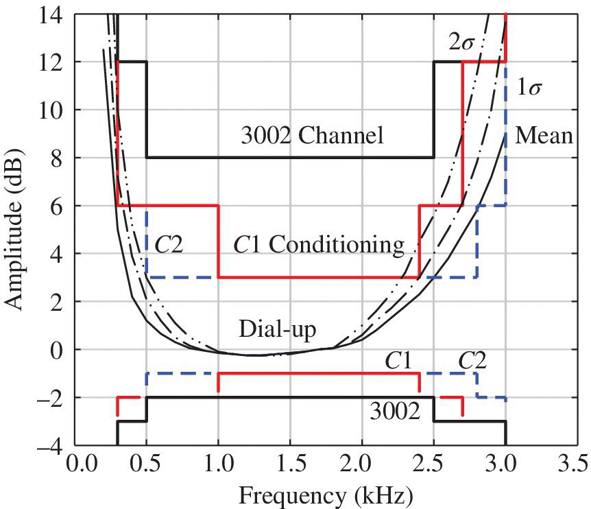
FIGURE 17.9 Dial‐up line amplitude characteristics for 3002 connection with C1 and C2 conditioning.

FIGURE 17.10 Dial‐up line delay characteristics for 3002 connection with C1 and C2 conditioning.
The one‐sigma amplitude and delay for the dial‐up channel corresponds approximately to the 3002 channel so that about 84% for the dial‐up connections are within the 3002 channel boundaries. In the following computer simulation examples, a fifth degree polynomial is curve‐fit to the C1‐conditioned amplitude boundaries and the resulting response is considered to be representative of a randomly selected C1‐conditioned channel. The phase response used in the simulations is based on a quadratic delay characteristic as discussed in Section 17.8.2.
17.8.2 Quadratic Delay (Cubic Phase) Function
The expression for the cubic phase function centered about the center frequency of the channel is given by
and the corresponding quadratic delay function is given by

The constants ![]() and
and ![]() are defined in terms of a specified delay at the channel band edge, B, so that
are defined in terms of a specified delay at the channel band edge, B, so that
and

where Fd1 and Fd2 are the normalized delays at the band edge for the quadratic and cubic phase terms, respectively. Substituting these results into the channel phase and delay functions and recalling that ![]() , results in the following normalized expressions
, results in the following normalized expressions


Computer simulations are used to demonstrate the distortion associated with the C1 line characteristic, using the pulsed modulated carrier input signal. The conditions are identified in Table 17.2 with the following exceptions: fc = fs = 1.7 kHz, Fd = 0, and Rs = 1.0 ksps. The signal distortion through an all‐pass filter with a linear phase response is examined in Problem 4. The various responses to the pulse modulated carrier are shown in Figure 17.11. Figure 17.11a shows the curve‐fit amplitude and the quadratic channel delay responses relative to the signal spectrum. Figure 17.11b shows the carrier modulated response and the corresponding magnitude function, and Figure 17.11c shows the I/Q responses. The concave upward, or smiling, characteristic of the quadratic delay distortion results in predominately post ISI terms. Figure 17.12 shows the same sequence of plots for a concave downward, or frowning, quadratic delay distortion. It is seen that the frowning quadratic delay distortion simply flips the response in time with the distortion appearing as mostly presymbol interference. Channel equalizers must be capable of equalizing both presymbol and postsymbol interference.

FIGURE 17.11 Response to C1 conditioned channel (Fd2 = 5.0).

FIGURE 17.12 Response to C1 conditioned channel (Fd2 = −5.0).
17.8.3 Practical Interpretation of the Phase Function
The phase functions used for the dial‐up channels are representative of the physical channels over certain regions of the frequency response. Suppose, for example, the actual phase function of the channel is similar to that shown in Figure 17.13. This satisfies the condition that the phase function has odd symmetry in frequency.

FIGURE 17.13 Example channel phase response.
Suppose now that this phase function is expressed as
Expanding (17.62) in a Taylor series about ωc gives
where
and
and
and
When these results are expressed in terms of the lowpass argument u = ω − ωc the phase function becomes
with
and
Upon substituting (17.64) through (17.67) into (17.70), the phase function is expressed as

and the corresponding delay function is

As an example of the cubic phase function, let ![]() and neglect powers of u greater than three so that (17.71) becomes
and neglect powers of u greater than three so that (17.71) becomes

Upon equating coefficients and considering Fd1 = 0, this result is identical to the cubic phase function used in Section 17.8.2. In a similar manner, the quadratic phase function is obtained when ![]() . Therefore, the phase characteristics outlined in Section 17.8.2 can be approximated by considering selected regions of a realizable channel phase function. In general, more complex phase functions can be realized using a Fourier series representation involving more terms.
. Therefore, the phase characteristics outlined in Section 17.8.2 can be approximated by considering selected regions of a realizable channel phase function. In general, more complex phase functions can be realized using a Fourier series representation involving more terms.
ACRONYMS
- AWGN
- Additive white Gaussian noise
- BPSK
- Binary phase shift keying
- HF
- High frequency
- I/Q
- Inphase and quadrature phase
- ISI
- Intersymbol interference
- VLF
- Very low frequency
PROBLEMS
- Referring to (17.4), show that Hr(ω) and Hi(ω) must be, respectively, even and odd functions of ω for h(t) to be a real function.
- Referring to (17.6) and (17.7) show the even and odd conditions of Hc(u) and Hs(u) with respect to their arguments that result in either hc(t) = 0 or hs(t) = 0.
- Show that the integration in (17.5) results in the I/Q lowpass filter functions hc(t) and hs(t) as expressed in (17.6) and (17.7). Then, using these results, show that the second equality in (17.5) applies.
- For a pulse signal input expressed as s(t) = Arect(t/T), compute the output response of a unit‐gain all‐pass filter with a linear phase response
 . Does the out signal experience any distortion?
 - Part 1: Derive the expression for the spectrum of the signal in (17.31) at the output of a unit‐gain all‐pass channel with the phase function expressed as
 .
.
Part 2: Sketch the three‐dimensional spectrum (see Figure 17.4) of the filtered signal obtained in Part 1. Show the horizontal ω axis and the orthogonal axes Re{S(ω)} and Im{S(ω)}. Label all pertinent parameters including A, T, ωs, τ, and ϕ.
Part 3: Evaluate the expression for the equivalent lowpass signal sc(t).
- Given the complex frequency translation of the channel input shown in Figure 17.3, express the frequency translated baseband signal
 in terms of the quadrature components sc(t) and ss(t) for the BPSK modulated input signal s(t) expressed in (17.31). Using the expression for
  in terms of sc(t) and ss(t) that you have just developed, show that the first equally in (17.32) applies.
 - Repeat Problem 5 for the QPSK modulated signal using the isolated symbol with ds = 1.
REFERENCES
- 1. R.W. Lucky, J. Salz, E.J. Weldon, Principles of Data Communication, McGraw Hill Book Company, New York, 1968.
- 2. A.A. Alexander, R.M. Gryb, D.W. Nast, “Capabilities of the Telephone Network for Data Transmission,” Bell System Technical Journal, Vol. 39, p. 431, 1960.
- 3. Bell System Technical Journals on Conditioned Lines, American Telephone and Telegraph Company, Bedminster, NJ, June 1969–1971.
- 4. E.D. Sunde, “Theoretical Fundamentals of Pulse Transmission‐I,” Bell System Technical Journal, Vol. XXXIII, No. 3, pp. 721–788, May 1954.
- 5. H. Urkowitz, “Bandpass Filtering with Lowpass Filters,” Journal of the Franklin Institute, Vol. 276, No. 1, July 1963.
- 6. J. Dugundji, “Envelopes and Pre‐Envelopes of Real Waveforms,” IRE Transactions on Information Theory, Vol. IT‐4, pp. 53–57, March 1958.
- 7. H.H. Skilling, Electrical Engineering Circuits, John Wiley & Sons, Inc., New York, 1958.
- 8. “1969–1970 Switched Telecommunications Networks Connector Survey (Reprints of Bell System Technical Journal Articles),” Bell System Technical Reference, PUB‐41007, April 1971.
- 9. “Data Communications Using the Switched Telecommunications Network,” Bell System Technical Reference, PUB‐41005, May 1971.