
3
DIGITAL COMMUNICATIONS
3.1 INTRODUCTION
A functional description of a communication system is shown in Figure 3.1. Generally the information source data is represented by discrete‐time and discrete‐amplitude digital data; however, if the information source is represented by continuous‐time and continuous‐amplitude analog data, then the source encoder includes time‐domain sampling and amplitude quantization. The resulting data is referred to as the source or user bit of duration Tb. Depending upon the nature of the data and the system performance requirements, the resulting digital information sequence may then undergo data compression. For example, if the information source is a facsimile system, then data compression is applied to eliminate redundant or unnecessary data or, in the case of voice data, the sampled voice signal is typically processed using a voice‐coding algorithm to minimize the required amount of data to be transmitted. The resulting source coded data sequence ![]() undergoes channel coding to mitigate impact of distortion on the received signal. Examples of channel coding are forward error correction (FEC) coding, data interleaving, and pseudo‐noise (PN) spread‐spectrum encoding. The FEC‐coded output consists of one digit per Tcb seconds where Tcb is the code‐bit duration. When direct‐sequence spread‐spectrum (DSSS) is applied each interval of duration Tc seconds is referred to as a chip. The channel coded data is then applied to the data modulator that assigns the resulting bits or chips to an amplitude and/or phase constellation that characterizes the transmitted symbol of duration T seconds.1 The modulator may interface at baseband with the transmitter; however, the interface commonly follows digital‐to‐analog conversion (DAC) and up‐conversion to an intermediate frequency (IF) on the order of 70 MHz. The functions of the transmitter provide frequency up‐conversion commensurate with the communication channel, power amplification, and spectral control; however, the more advanced waveform modulators include spectrally efficient waveforms that inherently satisfy specific transmit spectral masks. The transmit antenna plays a central role in establishing the directive power to establish the communication link. The functions following the channel perform the inverse of those just described, starting with the receiver antenna and ending with user data estimates provided to the information sink. However, these inverse functions are generally more complex and, in the case of the demodulator, more processing intense. The receive antenna interfaces with the receiver input low‐noise power amplifier (LNPA) and the subsequent frequency down‐conversion to the demodulator IF includes filtering for interference rejection and automatic gain control (AGC).2 Typically, the first tasks of the demodulator are to convert the IF input to baseband and provide analog‐to‐digital conversion (ADC) in preparation for the various functions of digital signal processing to accomplish signal acquisition, frequency, phase and symbol tracking, message synchronization, optimum symbol detection, and channel and source decoding to provide the best estimates of the source information.
undergoes channel coding to mitigate impact of distortion on the received signal. Examples of channel coding are forward error correction (FEC) coding, data interleaving, and pseudo‐noise (PN) spread‐spectrum encoding. The FEC‐coded output consists of one digit per Tcb seconds where Tcb is the code‐bit duration. When direct‐sequence spread‐spectrum (DSSS) is applied each interval of duration Tc seconds is referred to as a chip. The channel coded data is then applied to the data modulator that assigns the resulting bits or chips to an amplitude and/or phase constellation that characterizes the transmitted symbol of duration T seconds.1 The modulator may interface at baseband with the transmitter; however, the interface commonly follows digital‐to‐analog conversion (DAC) and up‐conversion to an intermediate frequency (IF) on the order of 70 MHz. The functions of the transmitter provide frequency up‐conversion commensurate with the communication channel, power amplification, and spectral control; however, the more advanced waveform modulators include spectrally efficient waveforms that inherently satisfy specific transmit spectral masks. The transmit antenna plays a central role in establishing the directive power to establish the communication link. The functions following the channel perform the inverse of those just described, starting with the receiver antenna and ending with user data estimates provided to the information sink. However, these inverse functions are generally more complex and, in the case of the demodulator, more processing intense. The receive antenna interfaces with the receiver input low‐noise power amplifier (LNPA) and the subsequent frequency down‐conversion to the demodulator IF includes filtering for interference rejection and automatic gain control (AGC).2 Typically, the first tasks of the demodulator are to convert the IF input to baseband and provide analog‐to‐digital conversion (ADC) in preparation for the various functions of digital signal processing to accomplish signal acquisition, frequency, phase and symbol tracking, message synchronization, optimum symbol detection, and channel and source decoding to provide the best estimates of the source information.

FIGURE 3.1 General functional diagram of a communication system.
Figure 3.1 serves as an outline of the subjects covered in this book. For example, a number of techniques for channel coding and decoding are discussed including the block and convolutional coding and their utility in different applications. Code concatenation, involving the application of several codes, has culminated in the powerful turbo codes (TCs) that perform very close to the theoretical coding limit introduced by Shannon [1] in 1948. The choice of waveform modulation is extremely important and establishes the transmission efficiency in terms of the number of bits/hertz and the spectral containment of the transmitter emission. A variety of digitally modulated waveforms are considered with applications to radio frequency (RF) transmission as in satellite communications and noncarrier or baseband transmission as used between many computer systems. The waveform demodulator is driven by the modulator selection and must perform a variety of functions for optimally detecting the received signal. In this regard, demodulator optimum filtering, carrier frequency and phase acquisition, and symbol synchronization and tracking are discussed in considerable detail. The ubiquitous channel is extremely important to understand and characterize to accurately design and predict the performance of communication systems. The channel characteristics and behavior are determined largely by the carrier frequency selection and channels ranging from very low frequency (VLF) to extremely high frequency (EHF) and optical frequencies are discussed and characterized. The waveform selection is also driven by the expected channel conditions. The most benign channel, and the easiest one to characterize, is the additive white Gaussian noise (AWGN) channel. In addition to its frequent occurrence in many applications, the AWGN channel forms the basis for comparing the performance of systems under more severe channel conditions. For example, the performance with selective and nonselective frequency fading is discussed, along with mitigation techniques, and compared to that of the AWGN channel.
In addition to the functional considerations of the system design as outlined in Figure 3.1, a heavy emphasis is placed on computer simulation results to characterize the communication systems performance. Computer simulations serve several essential functions: they provide a basis for the system performance evaluation in applications which defy detailed analysis, for example, evaluation of an entire communication link including complex channels and nonlinear acquisition and tracking functions; they provide a direct method for generating code for firmware and digital signal processor (DSP) implementations; they provide design and evaluation flexibility by means of relatively simple code changes; and, if properly written, they provide a form of self‐documentation throughout the code development.
Figure 3.2 shows a simplified application involving binary data from the information source occurring at a rate Rb = 1/Tb where Tb is the bit duration of the source information. In this example, the source data undergoes rate rc =1/2 FEC encoding resulting in a code‐bit rate of Rcb = Rb/rc = 2Rb. Assuming that a quadrature phase shift keying (QPSK) waveform is used to transmit the data over the channel, the function of the channel encoder is to map two consecutive code bits into one of four carrier phases resulting in a transmitted symbol rate of Rs = Rcb/2 = Rb. The symbol rate is important in that it must be compatible with the channel bandwidth requirements so as not to significantly distort the received signal and thereby degrade the detection performance.

FIGURE 3.2 A simplified example of source and channel encoding.
3.2 DIGITAL DATA MODULATION AND OPTIMUM DEMODULATION CRITERIA
Establishing an optimum decision rule involves multiple hypotheses testing of a statistical event given various statistical characteristics of the system model. The statistics generally involves a priori probabilities, transition probabilities, and a posteriori probabilities and the decision test involves minimizing the risk in the decision that involves choosing the event m given that the event m actually occurred. For example, if the decision is based on some measurement y, and the estimate of the actual event is characterized as ![]() , then it is desired to minimize the risk in saying that
, then it is desired to minimize the risk in saying that ![]() = m. This concept is shown in Figure 3.3 that depicts a space containing all possible hypotheses Hm of the events m: m = 0, …, M − 1 in the source. When the source events undergo a transformation to the decision space, the outcomes of the decisions represent estimates of the source events with associated probabilities of error. The transformation from the source to decision spaces can be viewed as source messages undergoing transmission over a noisy channel and, after some manipulation, interpreted by the receiver as to what message was sent. The receiver must have a priori knowledge, that is, know in advance that the messages will occupy unique decision regions in a noise‐free or deterministic transformation. The probabilities
= m. This concept is shown in Figure 3.3 that depicts a space containing all possible hypotheses Hm of the events m: m = 0, …, M − 1 in the source. When the source events undergo a transformation to the decision space, the outcomes of the decisions represent estimates of the source events with associated probabilities of error. The transformation from the source to decision spaces can be viewed as source messages undergoing transmission over a noisy channel and, after some manipulation, interpreted by the receiver as to what message was sent. The receiver must have a priori knowledge, that is, know in advance that the messages will occupy unique decision regions in a noise‐free or deterministic transformation. The probabilities ![]() are referred to as transition probabilities and represent the transformation from the source to the decision space as shown in Figure 3.3. Associated with each hypothesis there is also a probability P(Hi) representing the probability that the source event Hi will occur among all of the possible events; this probability is called the a priori probability of the source event.
are referred to as transition probabilities and represent the transformation from the source to the decision space as shown in Figure 3.3. Associated with each hypothesis there is also a probability P(Hi) representing the probability that the source event Hi will occur among all of the possible events; this probability is called the a priori probability of the source event.

FIGURE 3.3 M‐ary hypothesis testing.
For the M‐ary hypotheses the risk of a decision is defined as the weighted summation of probabilities, expressed as
where P(i|j) are the transition probabilities and represent the probability of event i when event j actually occurred. The transition probabilities correspond to an error event when i ≠ j and a correct decision is made when i = j. The probabilities P(j) represent the a priori probabilities of the individual events. The weights Cij represent costs associated with the corresponding decisions. In communication systems the emphasis is placed on minimizing errors so an error event is given the highest cost corresponding to Cij = 1 when i ≠ j and Cij = 0 when i = j. Under these conditions, the risk represents the overall system error probability and is expressed by the total probability law,
In the following analysis, the multiple hypothesis error criteria are applied to a communication system and, in the process, the requirements for making a decision that minimizes the overall error, as expressed by (3.2), are established. Consider, for example, that the source information has undergone source and channel coding resulting in contiguous M‐ary symbol messages νi = m as shown in Figure 3.4. Based on the earlier discussion, the a priori probability of a message is defined as
and the system error probability is characterized as

FIGURE 3.4 Waveform transmission with AWGN channel.
Applying the total probability law, the error is expressed as

The probability that ![]() is simply the integral of the probability density function (pdf) of the received signal taken over the decision region for the message event m and is expressed as
is simply the integral of the probability density function (pdf) of the received signal taken over the decision region for the message event m and is expressed as

so the error becomes

The error is minimized by maximizing the integrand, or the summation under the integral, and is expressed as

Therefore, the optimum decision rule is simply
This rule states that given the message m was transmitted the correct decision is made by choosing the message estimate ![]() that minimizes the error. However, at the demodulator the test statistic y is available, so the optimum decision must be based on y alone. To facilitate the use y, the decision rule can be reformulated into the desired result by applying a mixed form of Bayes rule to obtain the a posteriori probability of message m given by
that minimizes the error. However, at the demodulator the test statistic y is available, so the optimum decision must be based on y alone. To facilitate the use y, the decision rule can be reformulated into the desired result by applying a mixed form of Bayes rule to obtain the a posteriori probability of message m given by

This result states that the probability of declaring message m, given the test statistic y, can be accomplished through the demodulator processing by substituting (3.10) into the decision rule (3.9) resulting in the reformulated decision rule

The second equality in (3.11) is the formal characterization of the maximum a posteriori (MAP) decision rule; however, because p(y) is simply a constant, independent of the message, it does not influence the selection of the maximum value so the second equality corresponds to the decision rule given by (3.9), thus confirming that y is a sufficient statistic for making an optimal decision.
The MAP decision rule explicitly involves the a priori probabilities Pm; however, if the messages are equally likely, so that ![]() for all m, the decision rule is referred to as the maximum‐likelihood (ML) rule. The ML decision rule is expressed as
for all m, the decision rule is referred to as the maximum‐likelihood (ML) rule. The ML decision rule is expressed as

The decision rules can be formulated in terms of the likelihood ratio test (LRT) defined as

for which the MAP decision rule is
The logarithm is a monotonically increasing function of its argument and because the logarithm of the likelihood ratio often leads to a more intuitive result, the decision rule is also conveniently characterized in terms of the log‐likelihood ratio test (LLRT) as

3.2.1 Example Using Binary Data Messages
As an example of the application of the decision rules, consider the binary hypothesis test defined as
- H0: message m = 0, with a priori probability P(H0) = P0
- H1: message m = 1, with a priori probability P(H1) = P1
The message is transmitted over an AWGN channel as indicated in Figure 3.5.

FIGURE 3.5 Binary message with AWGN channel.
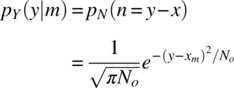
In this description, the channel is formulated as a simple vector channel and does not refer to a waveform type. For this characterization of the channel, the noise power is specified in terms of the one‐sided noise spectral density No (watts/hertz) and is consistent with the vector characterization of the signal in terms of the signal energy‐per‐symbol E (watt‐second). Because of the zero‐mean additive Gaussian noise channel, the pdf of the received vector is3
Based on the MAP decision rule, ![]() is chosen iff
is chosen iff ![]() and, using the likelihood ratio
and, using the likelihood ratio ![]() , the optimum decision is formulated as
, the optimum decision is formulated as

Therefore, using the pdf for Y, the LRT becomes

The utility of the log‐likelihood ratio (LLR) is evident in forming the LLRT test for the AWGN channel that results in the optimum decision rule

Solving (3.19) in terms of the test statistic y gives the useful result for the MAP decision rule, with respect to the threshold yt, expressed as

With equally probable messages and antipodal signaling, that is, with P0 = P1 and X0 = −X1, the decision threshold with respect to the origin of the x,y plane is shown in Figure 3.6a. The effect of different a priori probabilities tends to bias the threshold away from the message with the higher probability of occurrence.

FIGURE 3.6 Optimum decision boundary for binary detection processing.
For this example involving binary messages, the error probability is expressed as
Using the decision threshold yt, the individual error probabilities are evaluated as

and

Changing variables in these integrals by letting ![]() and recognizing that the integral is simply the probability integral4 for the Gaussian pdf results in the expressions
and recognizing that the integral is simply the probability integral4 for the Gaussian pdf results in the expressions


Upon evaluating ![]() for each message state, it is found that
for each message state, it is found that


and substituting these results into (3.24) and (3.25) gives


Defining the distance between the two modulated signals as ![]() these results simplify to
these results simplify to


A particularly simple expression results for the ML detection case with P1 = P0 = 1/2. In this case, the conditional‐error probabilities given by (3.30) and (3.31) are equal and the total‐error probability becomes

where Pbe denotes the bit‐error probability resulting from the binary message source, that is, each message represents a sequence of binary information bits. Recall that the modulator being considered in this example corresponds to ![]() and
and ![]() so the squared distance is
so the squared distance is ![]() , where the energy represents the energy‐per‐bit (Eb), and (3.32) is expressed as
, where the energy represents the energy‐per‐bit (Eb), and (3.32) is expressed as

The relationship to the complementary error function erfc(•) is discussed in Section 3.5. The argument Eb/No is the signal‐to‐noise ratio measured in a bandwidth equal to the data rate Rb = 1/Tb.
An interesting variation of the modulator can be examined by representing the squared distance in terms of the normalized correlation coefficient (ρ) between the two modulated messages as [2]
where ![]() and ρ is defined as
and ρ is defined as
Upon using these results with ![]() the bit‐error probability becomes
the bit‐error probability becomes

When ![]() the modulated signals are antipodal as in the preceding example; however, for
the modulated signals are antipodal as in the preceding example; however, for ![]() the signals are orthogonal and the bit‐error probability is degraded by 3 dB as seen from
the signals are orthogonal and the bit‐error probability is degraded by 3 dB as seen from

The bit‐error probability is plotted in Figure 3.7 as a function of the signal‐to‐noise ratio Eb/No, expressed in dB, for antipodal and orthogonal signaling.

FIGURE 3.7 Bit‐error performance for antipodal and orthogonal binary signaling.
3.3 INFORMATION AND CHANNEL CAPACITY
In this section a quantitative definition of information is introduced [1] and applied to a data source and, after passing through a discrete memoryless channel (DMC), the information content at a data sink is evaluated. The DMC channel is shown in Figure 3.8 and is characterized as having a fixed number of input and output letters Xi and Yi: i = 0, …, I − 1; j = 0, …, J – 1 with source probabilities PX(xi) and transitions from xi to yi defined in terms of the conditional probabilities PY|X(yj|xi). The conditional probabilities of the source data given the sink data are the a posteriori probabilities, denoted as PX|Y(xi|yj); these a posteriori probabilities are the performance measures to be optimized for i = j. The sink probabilities PY(yi) are of ancillary interest in the application of Bayes rule.

FIGURE 3.8 Discrete memoryless channel.
With the information content of the source data characterized in terms of the self‐information and average self‐information or source entropy, the remaining task is to define and characterize similar measures of information at the communication receiver or data sink when the source data is passed through the channel. The DMC channel is memoryless, in that, each channel use of a source letter xi is statistically independent of all the source letter uses. An example application of a DMC channel is the time and amplitude sampling of an analog signal s(t) such that t = iΔT where ΔT represents the discrete channel‐use interval and the finite number of discrete amplitudes samples, ΔAi, are represented by source letters xi = f(ΔAi).
The binary symmetric channel (BSC) channel, shown in Figure 3.9, is a special case of the DMC channel that uses binary input and output data, that is, the discrete amplitudes during each channel use have the form xi = {bi}: i = 0,1 with the natural bit mapping (b0, b1) = (0,1). In this case, the conditional probabilities PY|X(yi|xi) represent the channel transition probability defined as PY|X (yi|xi) = ε when j ≠ i and 1 − ε when j = i.

FIGURE 3.9 Binary symmetric channel.
The discrete‐time and amplitude analog signal samples, described earlier, can be applied to the BSC channel by quantizing the source samples into M = 2K discrete binary levels every ΔT seconds and then mapping each of the binary digits into a serial binary data sequence representing all of the discrete‐time source data samples. This technique is referred to a pulse code modulation (PCM) and the resulting bits are applied to the BSC channel as though originating from a binary data source.
The BSC channel capacity is defined as the maximum average mutual information between the source and sink data maximized over the a priori probabilities, PX(xi). In Section 3.3.1 the capacity of the BSC channel is evaluated using a binary source, and in Section 3.3.2 the results are extended to include an M‐ary source data. This section concludes by examining Shannon’s capacity limit for coded and uncoded waveforms using the Gaussian channel model.
3.3.1 Binary Symmetric Channel with Binary Data Source
Consider a binary data source X(xi) consisting of one information bit‐per‐channel use corresponding to K = 1 and M = 2. In the case xi = {bi}: i = 0,1 with the natural bit mapping (b0, b1) = (0,1). The self‐information contained in each bit is defined as

where the base‐2 logarithm is used specifically to denote binary data in bits of information,5 that is, K = 1 binary bit corresponds to M = 2K = 2 bit combinations giving rise to log2(2) = 1 bit of information. Note that (3.38) expresses the uncertainty of the source data, in that, for P(xi) approaching 1 the uncertainty, IX(xi), is nearly 1 and as P(xi) approaches 0 IX(xi) increases indicating more uncertainty. Because the source will generate either a binary 0 or 1, it follows from the total probability law that P(x0 = 0) + P(x1 = 1) = 1 so P(x0 = 1) = 1 − P(x1 = 0). Figure 3.10 shows the self‐information associated with each bit for 0 ≤ P(x1 = 1) ≤ 1, and it is seen that each source‐bit conveys one bit of information when each source‐bit is equally probable, that is, when P(x0 = 1) = P(x1 = 0) = 1/2.

FIGURE 3.10 Self‐information associated with one source bit.
The average self‐information is defined as the entropy of the source and is given by

As an example, suppose that a binary source generates the binary sequence xi = {0,1) and that it is required to evaluate the entropy of the source data for P(x1) = q: 0 ≤ q ≤ 1. In this case, M = 2 so (3.39) is evaluated as
This result is shown in Figure 3.11 and verifies that the maximum average self‐information or maximum entropy is one bit and occurs when the source bits are equally probable, that is, when q = 1/2.

FIGURE 3.11 Source entropy or average self‐information of Figure 3.10.
The mutual information corresponding to the source data xi and channel output or sink data yj is defined as

The mutual information can also be expressed in terms of the channel conditional transition probabilities between the sink and source data with the result

Because ![]() the probability space notation in (3.42) is changed to be consistent with the conditioning. The average mutual information is defined as
the probability space notation in (3.42) is changed to be consistent with the conditioning. The average mutual information is defined as

where the subscript ranges are i, j = 0,1. Substituting (3.42) into (3.43) with the change in notation gives

where
An alternate solution, and an easier solution to evaluate, is obtained by conditioning the mutual information, expressed by (3.41), on the sink data with the result

Using this result the average mutual information becomes
where the average self‐information of the source or the source entropy is given by (3.39) and the conditional entropy of the source given the sink data is evaluated as

Evaluation of (3.48) in terms of the source probability q and the BSC channel transition error probability ε results in
This result shows that, for binary source data, the conditional entropy of the BSC is independent of the a priori probabilities P(xi).6 The channel capacity is defined as the maximum average mutual information between the source and sink data maximized with respect to the a priori source data probabilities and is expressed as

Referring to Figure 3.11, the maximum source entropy, HX, corresponds to PX(xi) = 1/2 ∀ i and, using (3.49) for the conditional entropy, the capacity of the BSC channel is evaluated as
This result is plotted in Figure 3.12 as a function of the channel error. Referring to Figure 3.11 the maximum conditional entropy occurs under the condition ε = 1/2 corresponding to the most uncertainty in the received data. Not surprisingly, this also corresponds to condition for the least amount of information through the channel giving rise to the minimum channel capacity. The conditions corresponding to the minimum conditional entropy, that is, ε = 0 and 1, also correspond to the maximum channel capacity. While the definition of capacity does not distinguish between correct and incorrect data, if the data is known to be completely incorrect, ε = 1, then a correct decision can be made with certainty by simply reversing the decision. In practice, the bit‐error probability of an uncoded waveform will range between 1/2 and 1.0 as the signal‐to‐noise ratio increases from −∞ to ∞, thus limiting the practical range of the abscissas in Figure 3.12.

FIGURE 3.12 Channel capacity of BSC (K = 1, PX(xi) = 1/2).
3.3.2 Binary Symmetric Channel with M‐ary Data Source
In this section the channel capacity is evaluated when K binary digits of source data are transmitted during each channel use. For an arbitrary integer K this corresponds to xi = {biK−1, …, bi1, bi0}: bik ∈ (1, 0), k = 0, …, K − 1 where i = 0, …, M − 1 and M = 2K. By convention the least significant bit, b0, is on right‐hand side with the index i corresponding to the natural order of the binary bits, that is, x0 corresponds to = {0,…,0, 0), x1 corresponds to (0,…,0,1), and so on. The average self‐information of the M‐ary source data involves averaging over all of the M source data sequences and is computed as

Equation (3.52) is evaluated in terms of the source‐bit probabilities ![]() and
and ![]() with
with

It is easy to show (see Problem 4a and 4b) that the a priori probabilities of the M source sequences P(xi) are not all equal and that the summation of P(xi): i = 0, … < M − 1 is unity, that is,

so that each channel use necessarily corresponds to one of the source sequences. The thrust of this analysis and Problem 4 is to demonstrate that when the binary (1,0) source data probabilities are equal, that is, when q = 1 − q = 1/2 the source probabilities are identical and equal to P(xi) = 1/M ∀ i and that this condition results in the maximum source entropy.
Substituting (3.53) into (3.52) and summing over the M source sequences using the source bit probabilities q and 1 − q results in the following expression for the source entropy:

where the first term in the brackets denotes the binomial coefficients. By differentiating (3.55) with respect to q and setting the result equal to zero, the maximum source entropy is found to occur when q = 1/2 and the result is

From (3.55), the unique source bit a priori probabilities are
and the number of sources with probability P(xℓ) corresponds to the value of the binomial coefficient given in (3.56). With q = 1/2, (3.57) is ![]() and, considering the duplicated occurrences, this corresponds to
and, considering the duplicated occurrences, this corresponds to ![]() .
.
The conditional entropy of the source data, given the sink data, is evaluated using (3.48) by summing over the M source and sink sequences so that

The conditional entropy is evaluated using the same rationale as in the evaluation of the source entropy with the source‐bit probabilities P(![]() = 1) = q and P(
= 1) = q and P(![]() = 0) = 1 – q and the transition probabilities ε and (1 − ε) corresponding the BSC channel. Performing the summations in (3.58) with the appropriate source and sink sequences xi and yj the conditional entropy is evaluated as
= 0) = 1 – q and the transition probabilities ε and (1 − ε) corresponding the BSC channel. Performing the summations in (3.58) with the appropriate source and sink sequences xi and yj the conditional entropy is evaluated as

The final expression in (3.59) uses (3.54) so the condition entropy is independent of the a priori probabilities; this is explicit in (3.49) for the binary source case. Using (3.56) and (3.59) the average mutual information becomes

The capacity over the BSC with an M‐ary data source is evaluated as

Evaluation of (3.61) for ε = 1 and 0 using the limiting value xlog2(x) = 0: lim x → 0 results in the channel capacity C = K bits/use and the capacity at ε = 1/2 is found to be zero.
As an example application, consider the BSC channel with PX(xi) = 1/M: i = 0,…,M − 1. In this case the conditional entropy HX|Y and the capacity are plotted in Figures 3.13 and 3.14, respectively. The maximum conditional entropy occurs under the condition ε = 1/2 corresponding to the most uncertainty in the received data. Not surprisingly, this also corresponds to the condition for the least amount of information through the channel giving rise to the minimum channel capacity. The conditions corresponding to the minimum conditional entropy are ε = 0 and 1 that also correspond to the maximum channel capacity. Although the definition of capacity does not distinguish between correct and incorrect data, if the data is known to be completely incorrect, ε = 1, then a correct decision can be made with certainty by simply reversing the results. In practice, the bit‐error probability will range between 1/2 and 1.0 as the signal‐to‐noise ratio increases from −∞ to ∞, thus limiting the practical range of the abscissas in Figures 3.13 and 3.14.

FIGURE 3.13 Conditional entropy of BSC for K = 1, …, 4 (PX(xki) = 1/M).

FIGURE 3.14 Channel capacity of BSC for K = 1, …, 4 (PX(xi) = 1/M).
3.3.3 Converse to the Noisy‐Channel Coding Theorem
The converse to the noisy‐channel coding theorem has a very practical application that will be developed in Section 3.3.5. The application of interest is the characterization of the channel capacity for constrained data sources. That is, unlike Shannon’s unconstrained capacity limit, in this section, the channel capacity for a specified waveform modulation and coding is developed for the BSC channel. The converse to the coding theorem is related to concepts involving rate‐distortion theory and this introductory description focuses exclusively on the BSC channel and follows the more general and thorough description by Gallager [3].
The distortion measure for the BSC channel with source i = 0, …, M − 1 and sink j = 0, …, M − 1 is denoted as d(i,j) and is assigned a numerical value depending on the cost of the association between source xi and sink yj. For example, on the BSC channel with transition probability PY|X(yi|xi), the distortion measure assignment d(i,j) = 0 if i = j and =1 if i ≠ j. This notation indicates that the cost is zero for a correct decision and 1 for each incorrect decision. Assigning costs to various statistical decisions is a common practice in the performance optimization of both communications and radar system designs [4, 5]. The average distortion is defined as

and the rate‐distortion function of the source relative to a given distortion measure d′ is defined as
where IY,X is the average mutual information given by (3.60) for the BSC and R(d′) is the source rate relative to d′ with
The rate‐distortion function is a measure of the source capacity and, after considerable manipulations, is evaluated by Gallager (Reference 3, pp. 457–469) for a discrete memoryless source as

where d′ is the lower bound on the M‐ary source bit‐error to achieve the capacity C′. Equation (3.65) represents the converse to the channel coding theorem for a discrete memoryless source and the equality condition applies when
As stated previously, (3.65) and (3.66) will be applied in Section 3.3.5 to evaluate the theoretical capacity limits for multilevel pulse amplitude modulation (MPAM) and multilevel quadrature amplitude modulation (MQAM) modulated waveforms.
3.3.4 Shannon’s Channel Capacity Limit
The communications capacity through an AWGN channel is established by Shannon’s classical formula [6]

where W is the one‐sided bandwidth of the channel, Ps is the signal power, N = NoW is the total noise power, and No is the one‐sided noise power spectral density. Shannon’s capacity theorem states that, through proper coding and decoding design, error‐free transmission can be achieved through the AWGN channel for a communication source data rate Rb < C where C is the capacity of the channel in bits/second and that error‐free transmission cannot be achieved for Rb > C.
Shannon’s capacity limit applies to an unconstrained channel use, that is, it is not constrained by a particular type of waveform modulation. Although this channel capacity is unattainable in practice, except under the most ideal of circumstances,7 there are a number of coding techniques that are used together with waveform modulations that come very close to Shannon’s limit. For example, M‐ary coded waveforms and waveforms employing convolutional and block coding demonstrate the trend toward Shannon’s capacity limit. However, the most notable advances toward Shannon’s capacity limit have been in the area of TCs, turbo‐like codes, and low‐density parity‐check (LDPC) coding techniques; TC and LDPC codes are discussed in Sections 8.12 and 8.13. Shannon’s formula is used in Section 3.3.5, together with the converse to the coding theorem, to establish the capacity limit for various types of waveform modulations with coding.
Shannon’s capacity limit is interpreted in two distinct ways: the bandwidth limited interpretation and the power limited interpretation. In the bandwidth limited regime, the available channel bandwidth W is fixed and the capacity increases logarithmically with an increase in the signal power Ps, that is, the signal power must increase exponentially with the channel capacity. In this regime, the channel bandwidth is on the order of the information rate so improvements in the bit‐error probability is limited to increasing the signal power, providing waveform coding, within the confines of the channel bandwidth, and demodulator equalization; the wire‐line telephone channels are classical examples of fixed bandwidth channels. In the power limited regime, the signal power is a premium commodity and bandwidth abounds, that is, W ≫ Rb. In this case, the available bandwidth is used to provide M‐ary waveform coding and FEC coding to improve the bit‐error probability. The satellite communication channel is a classic example of operating in the power limited regime where power is very costly. Although Shannon’s capacity theorem provides performance limits in both regimes, in the power limited regime error‐free communications is approached with increasing bandwidth.
Shannon’s capacity in the bandwidth‐limited region is evaluated by normalizing (3.67), by the bandwidth W to obtain a measure of the channel efficiency expressed as

where γW = Ps/NoW is the signal‐to‐noise ratio measured in a bandwidth of W hertz. In this regime, the bandwidth W is fixed and the signal‐to‐noise ratio is increased by increasing the signal power Ps. Figure 3.15 shows the channel efficiency as defined by C/W as a function of γW. In this case, the number of degrees of freedom, based on the Nyquist bandwidth, is Nd = 2WT where T is the duration of the channel use. Shannon’s theoretical capacity, expressed by (3.67), applies for Nd = 2 degrees of freedom so W = 1/T is the bandwidth occupied by each channel use. For example, to transmit 4 bits/s/Hz through an AWGN channel requires a minimum signal‐to‐noise ratio of 12 dB using 2 degrees of freedom.

FIGURE 3.15 Shannon’s theoretical channel efficiency limit.
The BSC channel capacity can be applied when the channel errors result from AWGN simply by substituting ε = Pbe where

The solid line plots in Figure 3.16 show the results for K = 1, 2, and 3 bits‐per‐use (or bits‐per‐symbol) when plotted as a function of the signal‐to‐noise ratio Eb/No and interpreted as representing binary phase shift keying (BPSK), QPSK, and 8PSK waveform modulations, respectively. BPSK modulation uses only one of the two orthogonal dimensions in phase space, that is, only one channel of the in‐phase and quadrature (I/Q) baseband channels. Therefore, the fundamental capacity is limited to one half that of higher order phase modulated waveforms like QPSK and 8PSK that use both quadrature channels. The dashed curves in Figure 3.16 represent Shannon’s modulation independent or unconstrained maximum capacity for one‐ and two‐dimensional (1D and 2D) systems; Shannon’s capacity limit for coded modulation waveforms is discussed in Section 3.3.5. The detection loss of the M‐ary channel capacity relative to Shannon’s capacity measured at Eb/No = 2 dB is about 2.2 dB for each dimension. With multiphase shift keying (MPSK) modulation, prior to saturation at the capacity limit, the parameter K corresponds to a relatively high bit‐error probability condition so the gray and random decoding formulas8 for converting symbol errors to bit errors are not accurate. Consequently, the bit‐error performance results are obtained using Monte Carlo simulations to determine the 8PSK capacity performance in Figure 3.16.

FIGURE 3.16 MPSK capacity of AWGN channel for K = 1, 2, 3 (PX(xi) = 1/M).
In the power‐limited regime, the signal power is held constant and the bandwidth W is allowed to increase without limit. In this case, carrier‐to‐noise power density ratio, Ps/No, is constant and the capacity is evaluated as

This approximation requires that ![]() 9 so the communication is in a very low signal‐to‐noise environment. In this case, as the modulation coding uses more and more bandwidth the capacity increases linearly with the carrier‐to‐noise density ratio so bandwidth expansion through the use of coding is an effective way to approach the channel capacity limit. This result is based on a value of signal‐to‐noise ratio less than unity which is the case in a jamming environment so spread‐spectrum is an efficient use of bandwidth when the communication is being jammed.
9 so the communication is in a very low signal‐to‐noise environment. In this case, as the modulation coding uses more and more bandwidth the capacity increases linearly with the carrier‐to‐noise density ratio so bandwidth expansion through the use of coding is an effective way to approach the channel capacity limit. This result is based on a value of signal‐to‐noise ratio less than unity which is the case in a jamming environment so spread‐spectrum is an efficient use of bandwidth when the communication is being jammed.
In a period of time equal to T seconds, the maximum number of information bits that can be communicated under low signal‐to‐noise conditions is given by

where ![]() is the signal‐to‐noise ratio in the source information or bit bandwidth 1/Tb. Equation (3.71) can be viewed as having dimensions of bits/second/hertz in a bandwidth of W ≅ 1/T Hz so CT is also a measure of bandwidth efficiency. The rate of the coding, including the waveform symbol mapping, is defined as r = T/Tb ≅ Rb/W ≪ 1.
is the signal‐to‐noise ratio in the source information or bit bandwidth 1/Tb. Equation (3.71) can be viewed as having dimensions of bits/second/hertz in a bandwidth of W ≅ 1/T Hz so CT is also a measure of bandwidth efficiency. The rate of the coding, including the waveform symbol mapping, is defined as r = T/Tb ≅ Rb/W ≪ 1.
A commonly used performance measure is the ratio of the energy per information bit to the noise density, Eb/No, required to achieve a specified bit‐error probability Pbe. Upon letting C = Rb, the channel efficiency is expressed as

Defining the channel coding rate as10 r = Rb/W and solving (3.72) for Eb/No results in
This result is plotted in Figure 3.17 with Eb/No as the independent variable. The region r ≥ 1 represents the bandwidth‐limited region corresponding to modulation waveforms without coding like MPSK, MPAM, and MQAM. Typically M = 2K where K is the number of source bits mapped into an M‐ary signal amplitude and phase constellations. The channel efficiency of these modulated waveforms is included in Figure 3.17 corresponding a bit‐error probability of Pbe = 10−5; these performance data points are established in Chapters 4 and 6. On the other hand, the region corresponding to r < 1 represents the power‐limited region. Modulated waveforms having high coding gains and bandwidth requirements apply to this region.

FIGURE 3.17 Theoretical channel efficiency limit at Pbe = 10−5 (MQAM (squares), MPAM (circles), MPSK (triangles), M‐ary coded BPSK (diamonds)).
The Eb/No asymptote in the power‐limited region is determined by letting r → 0 in (3.73). Because the limit is indeterminate, the application of L’Hospital’s rule results in
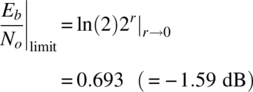
This is the theoretical limit in Eb/No for error‐free communications and is the target performance limit for coded waveforms. For example, for Eb/No > −1.59 dB there exists a coded waveform that will result in an arbitrarily small error probability. Conversely, for Eb/No < −1.59 dB there is no coding structure that will provide for an arbitrarily small error probability. Until the discovery of TCs [7] in 1993 the practical limit was on the order of 2–3 dB; however, with turbo coding Eb/No ratios below 0 dB have been achieved. Shannon’s capacity limit does not address the complexity associated with the decoding of low‐rate codes; however, prior to 1993 it was thought to be prohibitive; this notion was also overturned through iterative decoding, a hallmark of turbo decoding, resulting in reasonable computational complexity. As mentioned previously, TC, TC‐like codes, and LDPC codes are discussed in Chapter 8.
3.3.5 Capacity of Coded Modulated Waveforms
The channel capacity of an M‐ary data source with constrained waveform modulation, for example, MPAM, and MQAM, with coding over the BSC channel is evaluated using the rate‐distortion function characterized by (3.65) with source bit‐error probability corresponding the channel capacity given by (3.66). For the BSC channel, the maximum capacity occurs when PX(xi) = 1/M ∀ i so that the equality condition of (3.65) applies when ![]() . Therefore, using d′ = Pbe where Pbe is the bit‐error probability of the waveform modulation of interest corresponding to a prescribed signal‐to‐noise ratio Eb/No. With these conditions C′ is expressed as
. Therefore, using d′ = Pbe where Pbe is the bit‐error probability of the waveform modulation of interest corresponding to a prescribed signal‐to‐noise ratio Eb/No. With these conditions C′ is expressed as
The overall source rate r is defined as the ratio of the symbol rate (Rs) to the source bit‐rate (Rb) to the transmitted, that is,
The second equality includes the FEC coding rate rc = Rcb/Rb where Rcb is the rate of the FEC code bits and K = Rs/Rcb is number of code bits mapped into a transmitted symbol.11 Figure 3.18 shows the relationship between the source coding functions.

FIGURE 3.18 Source data coding rates.
For this evaluation Shannon’s capacity, expressed in terms of Eb/No, r, Nd and normalized by the bandwidth W = Rb/r, becomes

where Nd = 1 and 2 corresponding to the degrees of freedom. For example, in phase space, Nd = 1 corresponds using one of the quadrature phase channels as in BPSK modulation and Nd = 2 corresponds to using both the I and Q channels as in QPSK modulation.
For reliable communication, the code rate rc must satisfy the condition

where C′ is given by (3.65). Solving (3.78) for Eb/No under the equality condition results in
This result is plotted in Figure 3.19a for coded binary PAM (2PAM) with K = 1, M = 2 and, because pulse amplitude modulation (PAM) only uses one dimension of the carrier phase, Nd = 1. In this figure, and the following figures, the performance is plotted using the FEC code rate rc = r/K. The uncoded performance, shown as the dashed curves in the following figures, is included for comparison and is evaluated in Chapter 6. The results show the minimum Eb/No that can be obtained for a given code rate r and when r = 0 the FEC coding bandwidth is infinite and corresponds to Shannon’s limit of −1.59 dB. For this special case, the performance is identical to BPSK. Figure 3.19b shows the performance results using 4PAM with K = 2, M = 4, and Nd = 1. In this case, the theoretical limiting Eb/No values are considerably higher than with 2PAM coded modulation.

FIGURE 3.19 Performance limits of PAM with FEC coding.
Figure 3.20 shows the performance of coded 4QAM and 8QAM with K = 2 and 3 and the limiting performance with r = 0 corresponds to the Shannon limit. The 4QAM case is unique, in that, it also corresponds to the performance of coded QPSK modulation. The uncoded 8QAM performance curve, shown dashed, is based on a rectangular rest‐point constellation that is not an optimum configuration.

FIGURE 3.20 Performance limits of QAM with FEC coding.
Figure 3.21 is a summary of the minimum Eb/No as a function of the codulator rate r = Krc with modulation waveforms using Nd = 1 and 2 degrees of freedom. These maximum values correspond to Pbe = 0 so that C′ = K in (3.79). The limiting performance for r = 0 is Shannon’s limit of −1.59 dB. Because rc ≤ 1, values of r > 1 correspond to M‐ary modulated waveforms with M > 2.

FIGURE 3.21 Performance summary for Pbe = 0 (r = Krc).
3.4 BIT‐ERROR PROBABILITY BOUND ON MEMORYLESS CHANNEL
The analysis in Sections 3.3.1 and 3.3.2 characterizes the theoretical channel capacity of memoryless BSC channels in terms of the average mutual information as expressed in (3.61) for M‐ary modulated waveforms. In Section 3.3.5 the theoretical limit on Eb/No as a function of the code rate (rc) is examined for coded PAM and quadrature amplitude modulation (QAM) modulated waveforms. The results indicate that as rc approaches zero the limiting Eb/No approaches Shannon’s limit of −1.59 dB. However, these results do not establish the practical issue regarding the achievable capacity of a particular modulated waveform. An approach involving the computational cutoff rate (Ro) [8–11], defined in terms of the memoryless channel transition probabilities pY|X(yj|xi) introduced in Section 3.3, is used to examine this question.12 For example, using a n‐bit block coded waveform with n′ information bits with code rate Rc = rc = n′/n, the upper bound on the bit‐error probability for maximum‐likelihood decoding is expressed as
Equation (3.80) indicates that if Rc < Ro the bit‐error probability can be made arbitrarily small by increasing the code block size, otherwise an irreducible error event occurs.
The value of Ro for the BSC channel is listed in Table 3.1 [12] for hard‐ and soft‐decision detection of coherent BPSK and for binary, constraint length K, convolutional coding; this convolutional coded case requires that Ro/Rc > 1 to achieve an arbitrarily small bit‐error probability with increasing constraint length.
TABLE 3.1 Computation Cutoff Rate for Selected Waveforms.
| Waveform | Ro (Bits/Channel Use) | Comments |
| Coherent BPSK | Hard‐decision detectiona | |
| Coherent BPSK |  |
Soft‐decision detectionb |
a![]() for BSC channel with AWGN.
for BSC channel with AWGN.
bIn general, the exponent is Es/No where Es = kEb with k bits/symbol or channel use.
The computational cutoff rate is also applied in the design and evaluation of antijam (AJ) waveforms to counter jamming strategies [13–16]. In these descriptions the computational cutoff rate is conveniently characterized, in terms of the decoding metric D, M = 2k the modulation symbol states, and the code sequences of length n bits. The average bit‐error bound for pairs of code sequences of length n with randomly selected symbols is expressed as [17]

For (3.81) to conform to (3.80), such that ![]() , the computational code rate is defined as
, the computational code rate is defined as

Upon solving (3.82) for D results in
The upper bound on the bit‐error probability is defined in terms of parameter D as

For coherent BPSK modulation, corresponding to M = 2, with the AWGN channel and hard‐decision detection, the decoding metric is computed as [17]

Similarly, with soft‐decision detection,

For these binary cases, Ro is computed as

and (3.85) and (3.86) correspond to the respective conditions in Table 3.1.
The upper bound on the decoded bit‐error probability of the constraint length K, convolutional codes is expressed in terms of Ro as [11, 16]

Equation (3.88) applies for Ro > Rc. A more general bound, based on the channel coding and demodulator decision metric parameter D, is expressed as
where
The factor of 1/2 in (3.89) applies to all ML demodulation detection processing; typically this applies to antipodal and orthogonal modulated waveforms. The convolutional decoding function F′(D) is expressed as a polynomial in D, with ![]() . The polynomials in D are listed for constraint lengths 3 through 7 in Tables 8.29 and 8.30 for binary convolutional codes with rates 1/2 and 1/3 and in Tables 8.31 and 8.32 for rate 1/2 convolutional codes with 4‐ary and 8‐ary coding, respectively.
. The polynomials in D are listed for constraint lengths 3 through 7 in Tables 8.29 and 8.30 for binary convolutional codes with rates 1/2 and 1/3 and in Tables 8.31 and 8.32 for rate 1/2 convolutional codes with 4‐ary and 8‐ary coding, respectively.
Wozencraft and Jacobs [18] apply the computational cutoff rate as a measure to determine the bit‐error performance degradation with receiver quantization. In this case, a memoryless transition probability diagram is used to characterize L matched filter output levels and Q quantizer levels (Q > L) defining the transition probabilities ![]() ; q = 1, …, Q from which
; q = 1, …, Q from which ![]() is computed.
is computed.
3.5 PROBABILITY INTEGRAL AND THE ERROR FUNCTION
Evaluation of the bit‐error probability for a communication system in an AWGN channel is essential in determining the performance in the most basic of environments. One of the most important measures of the system performance is the signal‐to‐noise ratio Eb/No required to achieve a specified bit‐error probability. This performance measure is applied to most systems early in the design process even though the systems are ultimately to be used in vastly different environments like band‐limited channels and fading or impulsive noise channels. One reason for the characterization of the system performance in the AWGN channel is the simplicity associated with mathematical evaluations and the fidelity with which the channel noise can be implemented in the laboratory or modeled in computer simulations. Another reason is that AWGN is an underlying source of noise in almost all systems and must, therefore, be addressed at some point in the evaluation process. In this section various mathematical techniques are examined for describing the integral of the Gaussian pdf and clarifying various relationships between them and their application to system performance evaluations.
The Gaussian pdf is completely characterized by two parameters: the mean value (m) and standard deviation (σ) and is expressed as
A normalized form with zero mean and unit variance is obtained by letting y = (x − m)/σ for which p(y) is evaluated as

The probability integral is defined as

The complement ![]() is defined as
is defined as

The use of Q(Y) to denote the complement of the probability integral13 is used by Wozencraft and Jacobs [19] to characterize the bit‐error probability of a communication demodulator operating in an AWGN environment.
The error function [20, 21] and its complement are often used in place of Q(Y) to describe the bit‐error probability performance. These functions are defined as

and are depicted in Figure 3.22 in the context of the Gaussian pdf pY(y).

FIGURE 3.22 Depiction of error notations.
Unfortunately, there are several other definitions used for Q(Y), erf(Y), and erfc(Y). For example, Van Trees [22] uses the notation erf*(•) for P(Y) and erfc*(•) for Q(Y) and the error function and its complement are alternately defined as

In the literature these alternate definitions use identical notations; however, to avoid confusion they are distinguished in this text using the primed notation as in (3.96).
Using a simple substitution of variables these definitions are found to be related as

The error functions erf(Y) and erf′(Y) represent the area under the Gaussian pdf over the interval (−Y < y ≤ Y) about the mean value so that one half of the complementary error function corresponds to the complement of the probability integral, that is,

and it follows that

A polynomial approximation to the error function erf(Y), defined by (3.95), is attributed to Hastings [23], and expressed (Reference 20, Equation 7.1.26, p. 299) as

where p = 0.3275911, a1 = 0.254829592, a2 = −0.284496736, a3 = 1.421413741, a4 = −1.453152027, and a5 = 1.061405429. Over the indicated range of Y the approximation error is |ε(Y)| ≤ 1.5 × 10⁻⁷. Although (3.100) is used extensively in this book to compute the error function, more current applications use the VAX/IBM© intrinsic functions erf(x) and erfc(x) available with 32‐, 64‐, and 128‐bit precision [24].
ACRONYMS
- ADC
- Analog‐to‐digital conversion
- AGC
- Automatic gain control
- AJ
- Antijam (waveform)
- AWGN
- Additive white Gaussian noise
- BPSK
- Binary phase shift keying
- BSC
- Binary symmetric channel
- DAC
- Digital‐to‐analog conversion (or converter)
- DMC
- Discrete memoryless channel
- DSP
- Digital signal processor
- DSSS
- Direct‐sequence spread‐spectrum (waveform)
- EHF
- Extremely high frequency
- FEC
- Forward error correction
- I/Q
- Inphase and quadrature (channels or rails)
- IF
- Intermediate frequency
- LDPC
- Low‐density parity‐check (code)
- LLRT
- Log‐likelihood ratio test
- LNPA
- Low‐noise power amplifier
- LRT
- Likelihood ratio test
- MAP
- Maximum a posteriori (decision rule)
- ML
- Maximum likelihood (decision rule)
- MPAM
- Multilevel pulse amplitude modulation
- MPSK
- Multiphase shift keying
- MQAM
- Multilevel quadrature amplitude modulation
- PAM
- Pulse amplitude modulation
- PCM
- Pulse code modulation (baseband)
- PN
- Pseudo‐noise
- PSK
- Phase shift keying
- QAM
- Quadrature amplitude modulation
- QPSK
- Quadrature phase shift keying
- RF
- Radio frequency
- TC
- Turbo code
- VLF
- Very low frequency
PROBLEMS
- Show that the average conditional information or conditional entropy for the BSC with binary source data given by of (3.48) is independent of the source a priori probabilities. Using this result verify mathematically that the maximum capacity, shown in Figure 3.12, occurs when the source a priori probabilities are equal.
- Determine the self‐information and entropy for the source data sequences consisting of all possible combinations of K = 2 bits of binary data xi = {b1,b2}: bℓ ∈ {1,0}, ℓ = 1,2 when each bit bℓ occurs with equal probability. Express the results in both bits and nats. When each bit bℓ occurs with equal probability, and for any positive integer K, show that the source entropy is equal to K bits.
- Consider that 8‐bit ASCII characters are randomly generated with equal probabilities for 1 and 0 bits. Furthermore, each 8‐bit character is preceded with a mark (b1 = 1) start bit and is terminated with a space (b10 = 0) stop bit. Determine the self‐information associated with each bit and the average self‐information of the 10‐bit sequence.
- Suppose that a data source associates two bits‐per‐symbol, that is, K = 2, M = 4, and xi = {b1,b2}: bℓ ∈ {1,0}, ℓ = 1,2 with the probability of each mark bit equal to P(bℓ = 1) = q: 0 ≤ q ≤ 1.
- Determine the probability of P(xi): i = 1, …, M in terms of q for all 2K combinations of xi.
- Show that
 .
. - Express the average self‐information in terms of q.
- Plot a graph of HX(q) for 0 ≤ q ≤ 1.
- What is the maximum entropy of the source data bits and at what value of q does the maximum occur?
- Show that
 .
. - For the BSC shown in Figure 3.9, express the sink state probabilities P(yj): j = 1,2 in terms of the source bit or a priori probabilities P(xi): i = 1,2 and the channel error ε. Sketch P(y1) as a function of P(x1) for ε = 0, 1/2, and 1. Under what condition is P(yj) = P(xi)? What is the relationship between the channel transition probability and the a posteriori probability P(xi|yj) under these conditions?
- Referring to (3.73) derive Shannon’s limit for the power‐limited channel, that is, shown that Eb/No = −1.59 dB as r → 0.
- Derive the relationship between erf′(Y) and erf(Y) given by (3.97).
- Derive the relationship between erf(Y) and erf(−Y) and plot or sketch erf(Y) for all Y.
- Repeat Problem 9 for erfc(Y) and erfc(−Y).
REFERENCES
- 1. C.E. Shannon, “A Mathematical Theory of Communication,” Bell System Technical Journal, Part I & II, Vol. 27, No. 7, pp. 379–423, July 1948 and Part III, Vol. 27, No. 10, pp. 623–656, October 1948.
- 2. J.G. Lawton, “Comparison of Binary Data Transmission Systems,” Cornell Aeronautical Laboratory, Inc., Sponsored by the Rome Air Development Center, Contract AF 30(602)‐1702, date unknown.
- 3. R.G. Gallager, Information Theory and Reliable Communication, Chapter 9, John Wiley & Sons, Inc., New York, 1968.
- 4. H.L. Van Trees, Detection, Estimation, and Modulation Theory, John Wiley & Sons, New York, 1968.
- 5. W.B. Davenport, Jr., W.L. Root, An Introduction to the Theory of Random Signals and Noise, McGraw‐Hill Book Company, Inc., New York, 1958.
- 6. C.E. Shannon, “Communication in the Presence of Noise,” Proceedings of the I.R.E., Vol. 37, No. 1, pp. 10–21, January 1949.
- 7. C. Berrou, A. Glavieux, P. Thitimajshima, “Near Shannon Limit Error‐Correcting Coding and Decoding: Turbo Codes,” Proceeding of ICC ’93, pp. 1064–1070, Geneva, Switzerland, May 1993.
- 8. C.E. Shannon, “Probability of Error for Optimal Codes in a Gaussian Channel,” Bell System Technical Journal, Vol. 38, pp. 611–656, May 1959.
- 9. R.G. Gallager, “A Simple Derivation of the Coding Theorem and Some Applications,” IEEE Transaction on Information Theory, Vol. IT‐11, pp. 3–18, January 1965.
- 10. J.M. Wozencraft, I.M. Jacobs, Principles of Communication Engineering, Chapter 6, John Wiley & Sons, New York, 1967.
- 11. A.J. Viterbi, J.K. Omura, Principles of Digital Communication and Coding, Chapter 2, McGraw‐Hill Book Company, New York, 1979.
- 12. J.M. Wozencraft, I.M. Jacobs, Principles of Communication Engineering, pp. 398, 399, John Wiley & Sons, New York, 1967.
- 13. J.K. Omura, B.K. Levitt, “A General Analysis of Anti‐jam Communication Systems,” Conference Record, National Telecommunications Conference, November 1981.
- 14. J.K. Omura, B.K. Levitt, “Coded Error Probability Evaluation for Anti‐jam Communication Systems,” IEEE Transactions on Communications, Special Issue on Spread‐Spectrum Communications, Vol. COM‐30, No. 5, pp. 896–903, Part 1 of Two Parts, May 1982.
- 15. M.K. Simon, J.K. Omura, R.A. Scholtz, B.K. Levitt, Spread Spectrum Communications, Volumes I–III, Computer Science Press, Inc., Rockville, MD, 1985.
- 16. R.L. Peterson, R.E. Ziemer, D.E. Borth, Introduction of Spread Spectrum Communications, Prentice Hall, Upper Saddle River, NJ, 1995.
- 17. M.K. Simon, J.K. Omura, R.A. Scholtz, B.K. Levitt, Spread Spectrum Communications, Volume I, Chapter 4, pp. 192–202, Computer Science Press, Inc., Rockville, MD, 1985.
- 18. J.M. Wozencraft, I.M. Jacobs, Principles of Communication Engineering, Chapter 6, pp. 386–405, John Wiley & Sons, New York, 1967.
- 19. J.M. Wozencraft, I.M. Jacobs, Principles of Communication Engineering, Chapter 4, pp. 245–266, John Wiley & Sons, New York, 1967.
- 20. M. Abramowitz, I.A. Stegun, Handbook of Mathematical Functions with Formula, Graphs, and Mathematical Tables, Applied Mathematics Series 55, U.S. Department of Commerce, National Bureau of Standards, Washington, DC, June 1964.
- 21. H. Urkowitz, “A Note on the Error Function,” Research Memorandum RM‐1, Philco Scientific Laboratory, Philco Corporation, January 31, 1961.
- 22. H.L. Van Trees, Detection, Estimation, and Modulation Theory, Chapter 2, p. 37, John Wiley & Sons, New York, 1968.
- 23. C. Hastings, Jr., Approximations for Digital Computers, Princeton University Press, Princeton, NJ, 1955.
- 24. Lahey Software Solutions, “Lahey/Fujitsu Fortran 95 Language Reference, Revision D,” Lahey Computer Systems, Inc., Incline Village, NV, 1998.