
14
MODEM TESTING, MODELING, AND SIMULATION
14.1 INTRODUCTION
Perhaps the most useful and certainly the most ubiquitous tool for evaluating any communication system is a good uniform number generator; a close runner‐up is a good Gaussian number generator. Once this tool is available, it is used in virtually every simulation program to perform a variety of tasks. These tasks include: random source‐data generation, pseudo‐noise (PN) sequence generation, generation of various types of fading channels, and additive white Gaussian noise (AWGN) generation. Various methods of generating uniformly distributed random numbers are discussed in the following paragraph. With this background, the generation of other forms of random variables is examined and subsequent examples of system simulations focus on their applications in accurately characterizing system performance.
In terms of network terminology, the communication link is used here to include all of the functions of the physical layer between a data source and a data sink as depicted in Figure 14.1. In this context the channel may include, for example, a satellite repeater or bent‐pipe that does not process the received uplink signal for information content. Also, whenever there is a linear relationship between the transmitter and channel filtering, it is often convenient to treat the cascaded response as one filter. When this is done, however, care must be taken in the manner that various noise sources are added throughout the system. For example, if the uplink includes adjacent channel interference, then the transmitter and satellite filtering must be included as separate filters. In general, it is necessary to model the system implementation as closely as possible to the real encounter.

FIGURE 14.1 Functional diagram of a typical communication systems simulation.
Figure 14.1 is intended to aid in the description of the functions involved in simulating the performance of a communication system. The various seeds are typically used to generate uniformly distributed random numbers from which Gaussian, Rayleigh, and other random processes are generated. Using the same seeds for repeated simulations guarantees that the random conditions are duplicated so that performance variation can be attributed to changes in various system parameters. The various functions shown in Figure 14.1 provide inputs to the performance measure function that computes and formats the desired outputs for assessing the overall system performance. Example outputs are: received signal‐to‐noise ratio, number of block or bit errors, block and bit‐error probability,1 phase, frequency, and symbol tracking loop conditions, matched filter sampled outputs, and estimated parameter values. Two significant advantages of system simulations are: the ability to evaluate the system performance using parametric condition to determine how gracefully the system degrades; the ability to alter system parameters like: demodulator bandwidths, noise generator seeds, and interference and channel conditions, and then perform otherwise identically repeated simulations to attribute the performance variations to the system parameter or changes in the random conditions. This latter advantage is also a major simulation software debugging tool, in that, by repeating the same noise conditions in the various simulation loops, if the performance measures do not agree exactly then there is a problem with the simulation code. Typically this involves arrays or parameters not being re‐initialized properly between successive simulations.
14.2 STATISTICAL SAMPLING
The first consideration in any Monte Carlo simulation [1] is to determine the number of Monte Carlo trials that are required to achieve a specified accuracy in the performance measure(s). Typically, the performance measure in a digital communication system is the received bit‐error probability; however, symbol, character, and message‐error probabilities are also used. Each Monte Carlo trial or event is independent of all others leading to the notion of Bernoulli trials [2]. Under these conditions, if the underlying probability of an event is given by p, then the probability of an event occurring k times in n independent trials is given by the binomial distribution

where q = p − 1. The coefficient in (14.1) represents the number of possible combinations of n things taken k at a time. This is referred to as the binomial coefficient and is evaluated as

where x! is the factorial of x. The binomial distribution characterizes the discrete random variable k as depicted, for example, in Figure 14.2 for n = 5 and p = 1/2.

FIGURE 14.2 Discrete binomial probability distribution (n = 5, p = 1/2).
14.2.1 Fixed‐Sample Testing Using the Gaussian Distribution
Referring to Papoulis [2] it is shown that for large values of n, such that ![]() , that (14.1) is approximated over the region
, that (14.1) is approximated over the region ![]() by2
by2
This is the DeMoivre–Laplace theorem [3] and the right‐hand‐side is recognized as the Gaussian distribution with mean value ![]() and variance
and variance ![]() . Upon defining the variable
. Upon defining the variable ![]() , the mean of the distribution p(x) is p and the standard deviation is
, the mean of the distribution p(x) is p and the standard deviation is ![]() so that
so that
Returning to the problem of determining the number of Monte Carlo trials to perform in a system simulation, consider the mean value p of the pdf p(x) to be the system bit‐error probability of interest. Then, after n trials or bits, the standard deviation in the estimation of p will be
Because the underlying distribution is Gaussian, this result states that after n Monte Carlo trials the estimate of p will be within p ± σ with a confidence of 68.26%. Stated another way, if repeated Monte Carlo simulations are performed with independent underlying Gaussian random variables, then 68.26% of the measurements will be within ±σ of the expected value p. Higher confidence levels are readily determined by evaluating, for example, the ±2σ or ±3σ limits that correspond to confidence levels of 95.45 and 99.93% respectively.
It is often required to determine the number of trials, such that, the resulting measurement error is within a specified confidence level. Suppose, for example, that p is to be estimated within a two‐sigma (±kσ: k = 2) confidence level of 95.45% and with an accuracy of ≤10% (η = 0.1). In this case, let 2σ = 1.1p and evaluate (14.5) for n with σ = 1.1p/2. In the following section, the accuracy and confidence of a Monte Carlo simulation are characterized in terms of the required number of trials, n, and the number of observed errors, e, in the simulation.
14.2.1.1 Number of Trials Based on Accuracy and Confidence of Test
When the system bit‐error probability is unknown it is reasonable to ask, “How many bits (trials) must be simulated before the performance can be adequately assessed?” The answer to this question is found in the context of the sampling criterion discussed in the previous section. For example, for a discrete randomly sampled process with all events having equal probabilities of occurrence p, the probability Po of observing k events in n trials is approximated by [4]

where erf′(x) is the error function defined in Section 3.5 as

The mean value of the density function is np and the parameter k is defined as k = np1 where p1 ≥ p is an upper bound on p corresponding to a specified measurement accuracy of ![]() . Using these results with
. Using these results with ![]() , the expression for Po in (14.6) becomes
, the expression for Po in (14.6) becomes

The parameter p1 upper bounds the true error probability p. Using (14.8) the sample size, n, of the test can be evaluated in terms of the specified accuracy (η) and confidence level, Po. The unknown probability p is approximated by the frequency interpretation p ≅ e/n, where e is the number of error events after n trials. In the following analysis the argument of the error function in (14.8) is defined as
The value of x defined in (14.9) is evaluated for a specified Po by applying Newton’s method [5] to determine the solution to f(x) = 0, where

The iterative solution is given by

where the iteration continues until an acceptable error in (14.10) is achieved, for example, when ![]() . The derivative of f(x) is evaluated as
. The derivative of f(x) is evaluated as
where Hn is the Hermite polynomial [5] and ![]() for all x. Having approximated the value of x, the number of events required to satisfy the conditions of the test is determined as
for all x. Having approximated the value of x, the number of events required to satisfy the conditions of the test is determined as

where the approximation applies when p ≪ 1 corresponding to low error probabilities. Using e = np, the number of allowable errors during the test is
Therefore, upon terminating the test after n events, the test fails if the number of errors exceeds e otherwise the test passes.3
As an example of the application of these results consider simulating the performance of a modem detection algorithm at a signal‐to‐noise corresponding to a bit‐error probability of p = 1 × 10⁻³ with a confidence of 99% (Po = 0.99) and an accuracy of 5% (η = 0.05) corresponding to an upper bound on the bit‐error probability of p1 = 1.05p. Using Newton’s method, the value of x is 2.326282 and the number of bits required by the simulation is n = 2,162,471 and the maximum number of allowable bit errors is 2,163. Figure 14.3 shows the number of error events as a function of the error probability Pe = p for various confidence levels with a test accuracy of 5%, that is, the test determines that the modem is operating with an error probability p with an accuracy of 1.05p. This analysis leading to the number of error events, shown in Figure 14.3, results in a measurement accuracy of 5% regardless of the error probability; so, for very low error probabilities, the accuracy is commensurately low but the number of trials becomes very large. For example, when trying to measure an error event with a probability of p = 10−9 with 5% accuracy requires a sample size of more than 1012 trials. These examples are based on extremely accurate test requirements and more practical specifications may require confidence levels on the order of 80–90% with accuracies on the order of 10, 30, or even 100%.

FIGURE 14.3 Required error events to achieve an error probability with 5% accuracy.
In all of these tests, it is assumed that the signal‐to‐noise ratio is established with sufficient precision so that the modem is operating at the desired bit‐error probability; however, the accuracy of the test is influenced by the ability to accurately measure the signal‐to‐noise ratio. When examining modems with forward error correction (FEC) coding, the decoded bit‐error performance is very sensitive to the signal‐to‐noise ratio. In these cases, it is often more practical to first test the uncoded error performance. In addition, FEC decoding results in bursts of errors that influence the test accuracy; the preceding and following analysis assumes independent random error events. In Section 14.2.2, the method of sequential testing is discussed that terminates a test that is bound to fail with considerably fewer trials.
The conditions in the preceding example ensure that the simulated event error probability is less than 1.05p; however, it may be desirable to have the measurement accuracy within ±0.05p. This additional precision will require simulating more events resulting in longer simulation times. To assess the impact of this requirement the probability

is evaluated with k1 ≥ k2. Substituting ![]() and
and ![]() results in
results in
where x is given by (14.9). In this case the previous analysis procedures can be used by computing an equivalent value of Po given by
where Po is the confidence level of the +xσ case corresponding to (14.8). For example, with ![]() the equivalent confidence level is Po = 0.995 and, using p = 1 × 10⁻³ and η = 0.05, as in the previous example, the value of x is computed as 2.573709 so the number of bits required by the simulation is 2,646,942 and the number of bit errors is 2647.4
the equivalent confidence level is Po = 0.995 and, using p = 1 × 10⁻³ and η = 0.05, as in the previous example, the value of x is computed as 2.573709 so the number of bits required by the simulation is 2,646,942 and the number of bit errors is 2647.4
Returning to (14.5) and the following examples, the sampling requirements can be easily characterized by using tabulated confidence levels or probabilities Po(x) given the scaled standard deviation x = koσ. Typically [6] Po(x) is tabulated for a unit standard deviation with x = ko. The confidence level is plotted in Figure 14.4 as a function of ko and applies to the cases +koσ and ±koσ as discussed above. The disadvantage in this approach is that these values must be input from tables or interpolated from curves, whereas, in the previous analysis they are computed based on a specified confidence level.

FIGURE 14.4 Confidence level dependence on scale factor ko.
Therefore, using a desired confidence level, ko is determined from Figure 14.4 and, following the above analysis, the standard deviation is computed as
Equating (14.18) and (14.5) and solving for the number of trails yields

and, from (14.14), the number of errors is

where the parameter ko is determined using standard probability tables or Newton’s method as discussed following Equation (14.9).
Frequently error bars of length koσ or ±koσ about the probability p are included to indicate the accuracy of the simulation; an example using error bars is shown in Section 14.6. During the initial stages of the modem design and simulation, rough estimates of the system performance are needed. In this case, a test accuracy of 100% (η = 1.0) with ko = 2 or 3 is recommended to reduce the number of simulation trials to ![]() . As the modem algorithms are debugged and optimized, the accuracy and confidence level of the tests can be tightened for the final performance evaluations. As a final comment, the simulation or test time is a function of the event‐rate (R) events‐per‐second and is given by Ttest = n/R seconds. It is very time‐consuming to establish the number of trials to satisfy the performance requirements at a specified probability, say p = 10−5, and then run the simulation or test for a range of probabilities, say for p = 10−1 to 10−5, using the same number of trials. This results in unnecessarily high accuracies at the lower error probabilities and can be avoided by terminating the simulation at each probability (p) when the number of event errors, as expressed in (14.14) and (14.20), is exceeded.
. As the modem algorithms are debugged and optimized, the accuracy and confidence level of the tests can be tightened for the final performance evaluations. As a final comment, the simulation or test time is a function of the event‐rate (R) events‐per‐second and is given by Ttest = n/R seconds. It is very time‐consuming to establish the number of trials to satisfy the performance requirements at a specified probability, say p = 10−5, and then run the simulation or test for a range of probabilities, say for p = 10−1 to 10−5, using the same number of trials. This results in unnecessarily high accuracies at the lower error probabilities and can be avoided by terminating the simulation at each probability (p) when the number of event errors, as expressed in (14.14) and (14.20), is exceeded.
14.2.1.2 Measurement Accuracy with Signal‐to‐Noise Ratio Degradation
A useful criterion, which results in shorter simulation run‐times, is to require that the corresponding signal‐to‐noise ratio be within some specified accuracy Δγb(dB). In effect, this condition provides for a relative measurement accuracy that increases as the error probability decreases. For AWGN the bit‐error probability for uncoded antipodal signaling is related to the signal‐to‐noise ratio ![]() as
as
The variation in the bit‐error probability is expressed as
Letting ![]() , the derivative in (14.22) is evaluated as
, the derivative in (14.22) is evaluated as

with the result

Considering ![]() and
and ![]() , (14.24) is expressed as
, (14.24) is expressed as

Figure 14.5 is plotted ΔPbe/Pbe in percent as a function of γb for various accuracies in the signal‐to‐noise ratio Δγb(dB). The required number of trials is shown as the solid curves in Figure 14.6 as a function of the bit‐error probability for the indicated confidence levels and decibel accuracy in the measurement of Eb/No. For comparison, the number of trials associated with achieving a fixed accuracy in Pbe is shown as the dashed curves in Figure 14.6. For low error probabilities, a saving of several orders of magnitude in test time is realized by specifying a fixed error in Eb/No.

FIGURE 14.5 Measurement accuracy versus signal‐to‐noise ratio for various signal‐to‐noise accuracies.

FIGURE 14.6 Required bits versus bit‐error probability for various confidence levels and accuracies.
14.2.2 Fixed‐Sample Testing Using the Poisson Distribution
The preceding description using the Gaussian approximation to the binomial distribution applies only when p1 = k/n is in the vicinity of ![]() around the mean value p. These conditions require that n ≫ 1, p ≫ 1, with the product np ≫ 1. In the preceding sections, it was assumed that this vicinity extended over two or three standard deviations. Furthermore, the Gaussian distribution extends over the range p1 = (−∞,∞) that does not apply to the positive probability values and the finite sample size being considered. To overcome the positive and finite limitations of the sample variable k, the binomial distribution is approximated by the Poisson distribution expressed as [7]
around the mean value p. These conditions require that n ≫ 1, p ≫ 1, with the product np ≫ 1. In the preceding sections, it was assumed that this vicinity extended over two or three standard deviations. Furthermore, the Gaussian distribution extends over the range p1 = (−∞,∞) that does not apply to the positive probability values and the finite sample size being considered. To overcome the positive and finite limitations of the sample variable k, the binomial distribution is approximated by the Poisson distribution expressed as [7]

This result applies for k on the order of np and does not require that np ≫ 1. A formal proof of (14.26) is provided by Feller [3]. The criterion for establishing the sample size and the number of event errors is based on hypothesis testing [8–10], where the hypothesis H0 corresponds to the event probability p0 and the hypothesis H1 corresponds to the event probability p1. In terms of the Poisson distribution, these hypotheses correspond to the discrete density functions5
and
14.2.2.1 Single‐Threshold Fixed‐Sample Testing
In this section, the Poisson distribution is applied to a fixed‐sample test that determines the acceptance and rejection probabilities of the system under test. This fixed‐sample test is similar to the Gaussian test, in that, the test is performed until all n samples are completed before a pass–fail decision is made.
The likelihood ratio (LR) for the Poisson distribution is defined as

and the test threshold is established based on the log‐likelihood ratio (LLR) evaluated as

The optimum threshold is determined by solving (14.30) for k with λP = 1, yielding

The probabilities under the two hypotheses H0 and H1 are depicted in Figure 14.7; where it is assumed that a modem is being tested for a bit‐error probability of p0. As previously defined p1 = (1 + η)p0, where η is the accuracy of the test, that is, for a test length of n‐bits, the modem fails and is declared bad if the number of bits‐errors (k) exceeds the threshold Thk. The various regions indicated in Figure 14.7 give rise to the acceptance and rejection probabilities associated with the test and two regions are identified for establishing the criterion for the test, they are:

and


FIGURE 14.7 Sequential test description.
The probabilities Pca and Pfa are respectively referred to as the confidence and significance levels of the test and are typically expressed in percent. In statistical parlance, the probability α is a type I error, or error of the first kind, that rejects hypothesis H0 when H0 is true and the probability β is a type II error, or error of the second kind, that accepts hypothesis H0 when H1 is true.
For production testing the specification of Pca and Pfa, or confidence and significance, depend upon the modem application and are typically agreed upon through a written contract. However, the respective values of 0.95 and 0.05 (95 and 5%) seem reasonable in noncritical applications or in situations where the receiver signal‐to‐noise has a build‐in margin. In applications where the modem is costly it may be re‐worked and/or re‐tested. Prior to performing production testing, the modem must undergo extensive engineering testing to demonstrate that the fundamental algorithms are working correctly. For example, experience has shown that a modem can exhibit very infrequent bursts of errors that obliterate the error probability over hours of testing that would not be detected during a short test of n bits. These situations can often be traced to algorithm designs and related signal processing issues like: overflow and truncation.
The single‐threshold Poisson test described above is evaluated and the performance is characterized in Figures 14.8 and 14.9 as a function of the product np0 for various accuracies of the test expressed in percent. These results apply to any value of p0 as long as the product np0 is held constant. The irregular or scalloped appearance of these curves results from the integer quantization of the threshold np0. To achieve a confidence level of 95% and a significance level of 5% requires an accuracy of 40% with an np0 product of 80; however, to achieve a significance level of 1%, a test accuracy 60% is required with about the same np0 product. In these examples, the number of bits required in the test of a modem bit‐error probability is n = 80/p0, so with p0 = 1 × 10⁻³ the test requires n = 80 K bits.

FIGURE 14.8 Single‐threshold correct‐acceptance probability.

FIGURE 14.9 Single‐threshold false‐acceptance probability.
For test accuracies of about 10% and less, the underlying distributions for p0 and p1 are so close together that it is impossible to achieve confidence levels greater than about 90% and significance level less than about 20%; this is depicted in Figure 14.10 with np0 = 300 with a 5% accuracy, that is, np1 = 315, and an threshold of 307. In this case, the maximum confidence level is about 80% and the minimum significance is 19.7% and these represent limiting values as np0 increases above 300.

FIGURE 14.10 Poisson distributions with 5% accuracy and np0 = 300.
14.2.3 Sequential Sample Testing Using the Binomial Distribution
Sequential‐sample testing [11, 12] makes a pass–fail decision at each sample ![]() throughout the test. If at any sample, the number of errors crosses either of two thresholds the system fails the test, otherwise, the test continues until all n samples are completed; after the completion of the n samples, the system is accepted as good. The sequential test has the capability of rejecting bad systems early in the testing cycle resulting in considerably shorter test times. Because pass–fail decisions are made at each sample beginning at n = 1 the preceding approximations to the binomial distribution do not apply and the exact expression, given by (14.1), must be used. The two thresholds, Th0 and Th1, are depicted in Figure 14.11 and computed using the bounded LR λB for the binomial distributions; the conditions are:
throughout the test. If at any sample, the number of errors crosses either of two thresholds the system fails the test, otherwise, the test continues until all n samples are completed; after the completion of the n samples, the system is accepted as good. The sequential test has the capability of rejecting bad systems early in the testing cycle resulting in considerably shorter test times. Because pass–fail decisions are made at each sample beginning at n = 1 the preceding approximations to the binomial distribution do not apply and the exact expression, given by (14.1), must be used. The two thresholds, Th0 and Th1, are depicted in Figure 14.11 and computed using the bounded LR λB for the binomial distributions; the conditions are:

FIGURE 14.11 Sequential test description.
In this case, the LR, under the hypotheses H0 and H1, is expressed as

Upon substituting (14.35) into (14.34) and taking the natural logarithm results in the bounded expression

Using the upper bound and solving for k leads to the linear equation for the upper threshold as a function of n′ expressed as
where

Similarly, using the lower bound results in the linear equation for the lower threshold
where

These decision boundaries are depicted in Figure 14.12 where the abscissa and ordinate intercepts are evaluated as

and

FIGURE 14.12 Pass–fail decision boundaries for sequential test.
The average number of samples is [11]

It has been proven [11] that one or the other threshold will be crossed with probability 1 as ![]() . However, it is common practice to limit the sampling and terminate the test when
. However, it is common practice to limit the sampling and terminate the test when ![]() where n, somewhat arbitrarily, is set equal to
where n, somewhat arbitrarily, is set equal to ![]() plus twice the size of the fixed‐sample test, as determined from Figure 14.6, with the same accuracy using either ΔPbe or Δγb. The horizontal solid line in Figure 14.12 corresponds to the average number of errors at the termination point n under the two hypotheses, that is,
plus twice the size of the fixed‐sample test, as determined from Figure 14.6, with the same accuracy using either ΔPbe or Δγb. The horizontal solid line in Figure 14.12 corresponds to the average number of errors at the termination point n under the two hypotheses, that is,
If the test crossed the horizontal solid line, the modem fails; however, if the test terminates at the solid vertical line at n, the modem passes.
Table 14.1 summarizes the test requirements for an example modem production acceptance test and the corresponding sequential test parameters. This test requires a bit‐error probability of Pbe = 10−3 at some specified signal‐to‐noise ratio. The test parameters are used to establish the pass–fail boundaries as shown in Figure 14.12 and the number of bit errors is recorded and plotted as a function of the number of received bits. In this case, referring to Figure 14.6, the fixed sample test under these conditions requires about 1.2 × 106 bits so the sequential test is terminated after n = ![]() +2 (1.2 × 10⁶) = 4.557 × 10⁶. If the recorded data crosses the lower boundary, including the vertical boundary at n, the modem passes with the prescribed confidence and significance levels otherwise the modem fails the test.
+2 (1.2 × 10⁶) = 4.557 × 10⁶. If the recorded data crosses the lower boundary, including the vertical boundary at n, the modem passes with the prescribed confidence and significance levels otherwise the modem fails the test.
TABLE 14.1 Sequential Sample Test Requirements and Parameters for Modem Testing
| Test Requirements | |
| p0 = 1 × 10⁻³ | H0: specified bit‐error probability |
| Confidence 95% | H0 |
| Significance 5% | H0 |
| η = 5% | Test accuracy |
| p1 = 1.05 × 10⁻³ | H1: p1 = p0 (1 + η/100)a |
| Test Parameters | |
| A = 1.0252 × 10⁻³ | Slope of decision boundaries |
| B = 60.287 | Upper boundary constant |
| C = −60.287 | Lower boundary constant |
| ko = 60.287 | Upper boundary ordinate intercept |
| Lower boundary abscissa intercept | |
| Average number of samples | |
| n = 4.557 × 10⁶ | Test termination samples |
If p1 is specified then compute the test accuracy.
14.3 COMPUTER GENERATION OF RANDOM VARIABLES
The generation of various types of random variables is paramount in the performance simulation of modems and the foundation of nearly all random variable generators is the uniform number generator. The most ubiquitous of the random variable generators is the Gaussian random number generator that is used to model receiver and modem input noise. In this context, the Gaussian noise generator is used to establish the receiver or modem signal‐to‐noise ratio against which the premier performance measures involving the modem error probability are evaluated. During the modem development it is a common practice to establish the modem performance in a back‐to‐back mode, that is, without a channel, where the modulator intermediate frequency (IF) output (or transmitter radio frequency (RF) output) is coupled directly to the demodulator IF input (or receiver RF input). In this configuration the modem performance is compared to theoretical performance curves under relatively ideal conditions like: oscillator phase noise, amplifier nonlinearities, intersymbol interference (ISI), and demodulator quantization noise will result in somewhat less than idea performance. With the exception of the quantization noise these transceiver and modem noise sources are modeled using specialized random number generators, for example, the ISI noise is influenced by the randomization of the source data that is generated using a binary uniform random data generator. To examine the modem performance through a communication channel, the channel is frequently modeled using an additive or multiplicative random number generator. For example, additive co‐channel or adjacent channel interference is modeled using randomly modulated signals and the implementation of a fading channel simulator is modeled as a Rayleigh or Ricean random process.
In the following sections, computer implementation of various random number generators is discussed. The random variable Ui is used to denote uniformly distributed random variables; Xi is used to denote Gaussian distributed random variables, including correlated Gaussian variables; Yi is used to denote other random variables and Zi is used to denote the summation of independent iid random variables. Additional insights regarding the generation and testing of random numbers can be found in the literature [13–15].
14.3.1 Uniform Random Number Generation
As mentioned above, the uniform random number generator forms the foundation for the generation of nearly all other random variables. The uniform number generator generates a sequence of random numbers that are ideally6 independent and uniformly distributed over the period of the generator; the period is determined by the computer’s internal processing size and the specific algorithm being used to generate the uniform numbers. Ideally the uniform numbers are characterized by the uniform pdf shown in Figure 14.13 where the range of the random numbers is a ≤ ui ≤ b with a mean value of (a + b)/2.

FIGURE 14.13 Uniformly distributed probability density function.
Random numbers that represent a continuous pdf p(u) with cumulative distribution ![]() are generated using uniformly distributed random numbers
are generated using uniformly distributed random numbers ![]() , i = 0, 1, … and the inverse function u = P−1(Ui). In these cases, the parameters a and b are: a = 0 and b = 1. To generate random bipolar binary source data, d = {−1,1} the same procedure is used, however, the cumulative distribution P(U) is a linear function of U and, using the parameters a = −1/2 and b = 1/2, the source data is generated as di = sign(1, Ui), where −1/2 ≤ Ui ≤ 1/2, i = 0, 1,… are uniformly distributed random numbers. This description discusses the characteristics and application of uniformly distributed random numbers; however, methods for generating and testing them7 [16] is the subject of the remainder of this section.
, i = 0, 1, … and the inverse function u = P−1(Ui). In these cases, the parameters a and b are: a = 0 and b = 1. To generate random bipolar binary source data, d = {−1,1} the same procedure is used, however, the cumulative distribution P(U) is a linear function of U and, using the parameters a = −1/2 and b = 1/2, the source data is generated as di = sign(1, Ui), where −1/2 ≤ Ui ≤ 1/2, i = 0, 1,… are uniformly distributed random numbers. This description discusses the characteristics and application of uniformly distributed random numbers; however, methods for generating and testing them7 [16] is the subject of the remainder of this section.
Computer language software often includes a function for generating uniformly distributed random numbers that presumably has been tested for various properties of randomness. The congruence method [13] or algorithm is commonly used for generating a sequence of random numbers ![]() where C is the magnitude of the maximum number as determined by the number of computer bits used to represent a number. Uniformly distributed random numbers
where C is the magnitude of the maximum number as determined by the number of computer bits used to represent a number. Uniformly distributed random numbers ![]() are determined as
are determined as ![]() .
.
The congruence method [13] is expressed as8
where B is chosen to be relatively prime to C and the constants A with B chosen to provide the desired random properties and the longest possible sequence of random numbers. The initial value, X0, is the generator seed and is selected to be relatively prime to C. Theoretically each seed produces an independent random sequence and a unique seed is assigned to the various simulation functions. For example, unique uniform number generator seeds are assigned to generate: additive Gaussian noise, phase noise, desired and interfering channel source data, and channel fading. Although the congruence method described by (14.45) provides excellent random properties and adequate sequence lengths, it is relatively slow compared to the implementation described by Knuth [17].
Finite‐length pseudo‐random sequences generated using maximal‐length sequences exhibit excellent random properties and nearly ideal correlation responses; these are often referred to as PN sequences or M‐sequences. PN sequences are introduced and discussed in Chapter 8.
Uniform random number generators and M‐sequences can be tested against several relatively simple criteria to verify that their performance characteristics satisfy the independence and random properties. The first test involves the autocorrelation response of the random sequence and the resulting power spectral density (PSD). For a sequence of length n, the autocorrelation response is a single sample with amplitude n and sidelobe levels on the order of 1/n. The PSD is determined by taking the Fourier transform of the correlation function that ideally corresponds to white noise characterized by a constant PSD frequency response. Correlation and PSD responses expose non‐random behaviors involving initial seed repetitions and the existence of repeated patterns that do not follow the definition of Bernoulli trials and the underlying binomial distribution. This suggests a second test involving the binomial distribution expressed by (14.1) with p = q = 1/2, that is, each binary event occurs with equal probability. In this case, the binomial distribution becomes
Considering a binary sequence of length n, consisting of mark and space data bits9 with respective probabilities p = q = 1/2, the binomial coefficients represent the number of times that k mark‐bits will occur in the data sequence and (14.46) is the corresponding probability of occurrence. For example, using a binary sequence of length n = 3 bits the binomial coefficients for k = 0, 1, 2, 3 are {1, 3, 3, 1} respectively. The binary data patterns are listed in Table 14.2 with the corresponding patterns containing k mark bits. The number of k mark‐bit patterns is consistent with the binomial coefficients and the corresponding probabilities of occurrence are {1/8, 3/8, 3/8, 1/8}. The Bernoulli trial test is a relatively simple test to perform.
TABLE 14.2 Binary Data Patterns in a Sequence of Length n = 3
| Data | k |
| 000 | 0 |
| 001 | 1 |
| 010 | 1 |
| 011 | 2 |
| 100 | 1 |
| 101 | 2 |
| 110 | 2 |
| 111 | 1 |
Other uniform number generator tests involve: examining the repetition of seeds during the sequence generation; sequence independence with different starting seeds; the length of the sequence; the periodic generation of subsequences. For example, when different starting seeds are applied to the generation of co‐channel and adjacent channel interference, it is important to ensure that the random properties of these channels are independent from each other and the desired channel. Also, when simulating the performance of modems using turbo‐coded FEC, run lengths of millions or perhaps billions of bits may be required so the length of the random sequence generators becomes important. Additional tests, involving the generation of uniform random numbers, must be performed to examine the generators’ ability to duplicate specific random processes within the prescribed confidence levels; examples using the exponential and Gaussian random processes are given in the following sections.
14.3.2 Gaussian Random Number Generation
The generation of Gaussian random numbers is a close runner‐up to uniform number generators in terms of its utility in modem performance simulations. Gaussian number generators use the inverse of the Gaussian cumulative distribution PG(X): 0 ≤ PG(X) ≤ 1 so, the uniformly distributed random number Ui: 0 ≤ Ui ≤ 1, forms the basis for the generation of Gaussian random numbers using ![]() . This is depicted in Figure 14.14 for a zero‐mean, unit standard deviation Gaussian distributed random number. Gaussian random numbers with mean (mx) and standard deviation (σx) are simply obtained as
. This is depicted in Figure 14.14 for a zero‐mean, unit standard deviation Gaussian distributed random number. Gaussian random numbers with mean (mx) and standard deviation (σx) are simply obtained as

FIGURE 14.14 Generation of Gaussian random numbers using inverse cumulative probability.
Although the inverse mapping ![]() of the Gaussian cdf describes the process for the generation of Gaussian random numbers, fast and efficient methods for their generation on computers are described by Muller [18]. The approach used in most of the simulation results presented in this book uses the approximation to the inverse function
of the Gaussian cdf describes the process for the generation of Gaussian random numbers, fast and efficient methods for their generation on computers are described by Muller [18]. The approach used in most of the simulation results presented in this book uses the approximation to the inverse function ![]() given by Hastings [19, 20], with an approximation accuracy of
given by Hastings [19, 20], with an approximation accuracy of ![]() . Hastings’ approximation for Gaussian number generation is given in Figure 14.15.
. Hastings’ approximation for Gaussian number generation is given in Figure 14.15.

FIGURE 14.15 Approximate Gaussian random number generation.
Abramowitz [5, p. 933]. Courtesy of U.S. Department of Commerce.
Gaussian random numbers can also be generated by summing independent random variables and recognizing that the central limit theorem [21, 22] applies. One approach is to sum uniformly distributed numbers Ui with the result ![]() where the distribution of Z approaches a Gaussian distributed random number as the number of summations approaches infinity. Another application of the central limit theorem is the summation of sinusoidal functions with uniformly distributed phase, that is, with −1 ≤ Ui ≤ 1 and
where the distribution of Z approaches a Gaussian distributed random number as the number of summations approaches infinity. Another application of the central limit theorem is the summation of sinusoidal functions with uniformly distributed phase, that is, with −1 ≤ Ui ≤ 1 and ![]() then
then ![]() and Z approaches a Gaussian distribution as the summation index increases.
and Z approaches a Gaussian distribution as the summation index increases.
The utility of the Gaussian number generator in simulating the modem bit‐error probability performance is determined by examining the number of simulation trials that fall within the confidence and accuracy limits given the required number of Monte Carlo samples‐per‐trial. The number of samples‐per‐trial is determined using (14.13) or the equivalent expression (14.19), repeated here as

where η is the specified confidence level of the Monte Carlo simulation and, using Figure 14.4, ko is determined as the corresponding standard deviation scale factor. This test is examined in the case study in Section 14.6 where it is demonstrated that the Gaussian random number generator, when used as a Gaussian noise source, performs within the expected statistical bounds of the bit‐error probability p = Pbe.
14.3.2.1 Correlated Gaussian Random Number Generation
Correlated Gaussian random numbers can be generated in several ways using Xi. For example, referring to Papoulis [23], the conditional distribution of a correlated Gaussian random variable Xi+1 with correlation coefficient ρ, mean value ρXi, and variance σ2, for i = 0, 1, … and X0 = 0, is expressed as

The various expectations of Xi are given by
and
where α = sin−1(ρ): −π/2 < α ≤ π/2. Upon generating a sequence of correlated Gaussian random samples, the correlation coefficient is computed from the normalized response of the autocorrelation function.
The correlated Gaussian random variables are also generated using the autoregressive (AR) model [24] expressed as

This is an N‐th order AR process where the current value, Zi, of the processes is a linear combination of the past N values plus an error term Xi characterized as independent Gaussian noise samples. The weights wj are determined as the solution to N simultaneous equations.
The method of generating correlated random variables using a defined PSD is discussed in Chapter 20. A classical method used to generate correlated random samples that characterize the Doppler spread of the channel is Jakes’ PSD function given by [25]

where f is the frequency around fd. An application using the phase PSD to generate inphase and quadrature samples for a Rayleigh fading channel is given in Section 20.7.
14.3.3 Ricean and Rayleigh Random Number Generation
Ricean random numbers Yi are generated using two zero mean independent iid Gaussian random variables XIi and XQi with standard deviation σr,
where Vs represents the received peak signal level or specular value of the received signal plus noise. Defining the specular to random signal‐to‐noise ratio as

and normalizing Yi by σr results in the normalized Ricean random variables

where ![]() and
and ![]() are zero‐mean unit‐variance Gaussian random variables. Rayleigh random numbers result when the specular to random power ratio approaches zero, that is, when
are zero‐mean unit‐variance Gaussian random variables. Rayleigh random numbers result when the specular to random power ratio approaches zero, that is, when ![]() and, in the limit (14.55), becomes
and, in the limit (14.55), becomes
Examples of Ricean and Rayleigh pdfs generated using (14.55) and (14.58) respectively are given in Section 18.2. Correlated Ricean and Rayleigh random numbers are obtained by using (14.49) in the generation of ![]() and
and ![]() . An example of the correlation characteristics for the Ricean random numbers generated with specular‐to‐random component ratio of γsr = 12 dB is shown in Figure 14.16. These results are obtained using a sequence of 5000 Ricean generated samples using (14.55) with the underlying correlated Gaussian random variables generated using (14.49).
. An example of the correlation characteristics for the Ricean random numbers generated with specular‐to‐random component ratio of γsr = 12 dB is shown in Figure 14.16. These results are obtained using a sequence of 5000 Ricean generated samples using (14.55) with the underlying correlated Gaussian random variables generated using (14.49).

FIGURE 14.16 Correlation response for correlated Ricean random numbers (γsr = 12 dB).
When these results are used in a system performance simulation, it is important to know the corresponding correlation time associated with the specified correlation coefficient ρ. The correlation interval is defined as correlation lag no where the correlation response equals the normalized correlation threshold of e−1. For example, for the case γsr = 12 dB, the correlation lag no is determined from Figure 14.16 as a function of correlation parameters ρ. The correlation lag characteristics are summarized in Figure 14.17 for the indicated values of γsr. The case γsr = −∞ corresponds to correlated Rayleigh random variables and as γsr → +∞ and the random variable Yi approaches the constant signal amplitude Vs. The decorrelation time is denoted as τo and is related to the sampling interval, Δτ, associated with the random variable Yi and is expressed as

FIGURE 14.17 Correlation interval for Ricean random numbers generated using Equation 14.57.
Fast fading environments are associated with signal fluctuations that are rapid relative to the transmitted symbol duration. Fast fading results in significant symbol distortion in the demodulator matched filter. Considering that a minimum of four samples‐per‐symbol is required to satisfy the Nyquist requirement with or without fading, the required sampling frequency is expressed as

The application of these results to communication system operating in a fading environment starts with the specification of the parameters T, τo, ρ, and γsr. Using ρ and γsr, the value of no is determined from Figure 14.17. The de‐correlation time is typically specified in terms of slow fading (τo ≥ NT) or fast fading (τo < NT), where the selection of N is somewhat subjective; choosing N = 1 results in a matched filter distortion loss, so values of three or four are preferable. Normally the specified range of τo is several orders of magnitude. The selection of Ns depends on the symbol spectral sidelobes and the specified aliasing distortion, however, Ns = 4 is frequently used. Based on these observations, the sampling frequency is selected using (14.60).
14.3.4 Poisson Random Numbers
The generation of Poisson random numbers is based on the pdf expressed as
Expressing the parameter α as ![]() , where τ ≥ 0 is the time between the Poisson distributed events, then (14.61) becomes
, where τ ≥ 0 is the time between the Poisson distributed events, then (14.61) becomes
As seen in the following section, the time interval between the Poisson distributed events is represented by the continuous exponentially distributed random variable τ that is used to generate the Poisson random variables.
14.3.5 Exponential and Poisson Random Number Generation
The generation of exponentially distributed random numbers uses the inverse probability mapping ![]() where the cumulative distribution
where the cumulative distribution ![]() and Ui: 0 ≤ Xi ≤ 1 is a uniformly distributed random number. Using the exponential pdf, given in Table 1.8 and expressed as,
and Ui: 0 ≤ Xi ≤ 1 is a uniformly distributed random number. Using the exponential pdf, given in Table 1.8 and expressed as,
the exponentially distributed random variables Yi are computed as

When simulating the performance of queuing systems [26] the random variable y represents the random time intervals Δτ between events in the queuing system and, in this application (14.64), is used to generate the time between the occurrences of events in the Poisson process. The exponential distribution is memoryless, in that, the past occurrences Yn: n = 0,…, i − 1 do not influence the prediction of Yi.10 Because Yi represents the interval between the occurrences of Poisson distributed events, the Poisson distributed random events or numbers are generated as

Using k as the summation limit is significant, in that, this is the same variable used in (14.62) to characterize the Poisson distribution. Papoulis [27] shows that there are exactly k events in the interval τ where, upon letting ![]() , τ = Zk. Plots of the theoretical pdf for Poisson distributed random variables are shown in Figure 14.18 for k = 0–4; it is left as an exercise (see Problem 14) to plot the corresponding pdfs for Poisson pseudo‐random variables generated using (14.64) and (14.65).
, τ = Zk. Plots of the theoretical pdf for Poisson distributed random variables are shown in Figure 14.18 for k = 0–4; it is left as an exercise (see Problem 14) to plot the corresponding pdfs for Poisson pseudo‐random variables generated using (14.64) and (14.65).

FIGURE 14.18 Theoretical pdf for the Poisson distributed random variables (λ = 1.0, k ≤ 4).
14.3.6 Lognormal Distribution
The lognormal distribution characterizes an impulsive noise communication channel in terms of the received noise amplitude x, expressed by
where x is a random variable for which the logarithm y = ln(x) is a normally distributed random variable, with mean m = E[ln(x)] = E[y] and variance ![]() . Using the random variable y, (14.66) is expressed as the Gaussian or normal distribution pY(y) given by
. Using the random variable y, (14.66) is expressed as the Gaussian or normal distribution pY(y) given by
The random variable x is exponentially related to y as11 x = ey and, unlike the Gaussian distribution, the lognormal distribution is skewed so that high values of x occur with relatively high probabilities as seen from the plots of (14.66) in Figure 14.19.

FIGURE 14.19 Theoretical pdf for the lognormal distributed random variables (mx = 0; σx2 ≤ 1, 0.5, 0.1).
Because of the impulsivity of the random variable x, the lognormal distribution is used to generate impulse noise that is characterized or measured in terms of the ratio of the rms envelope to average envelope defined as

The sampled lognormal noise appears at the input to the receiver and undergoes dispersion in the various receiver and modem filters. The filtering broadens the impulse response in time and simultaneously decreases impulsiveness resulting in a smaller value of Vd. For example, the limiting case of impulsive noise occurs when the noise energy, from worldwide storm activity, is randomly added and filtered resulting in Gaussian noise with a Vd value of 1.049 dB. The lognormal pdf is encountered in Section 19.10 as it relates to lightening‐induced impulsive noise in the VLF and LF communication channel.
14.4 BASEBAND WAVEFORM DESCRIPTION
With few exceptions,12 the simulation of communication systems involves a baseband characterization of the signal and channel. This characterization is embodied in the complex envelope, also referred to as the analytic signal representation of signals, channels, and various transmitter and receiver filters. The analytic signal representation is simply a baseband description of the signal that is obtained by a linear translation of a carrier‐modulated signal to baseband as found in heterodyne or homodyne receivers. Typically, baseband simulations are valid in situations involving low instantaneous bandwidths, B, relative to the carrier frequency (fc) that is, when B/fc ≪ 1. As in the case of establishing the Nyquist bandwidth of a signal, the bandwidth B must be defined with care. For example, with a rectangular modulated waveform the signal bandwidth is typically defined in terms of the equivalent noise bandwidth of the matched filter, that is, 1/T where T is the symbol duration. However, the resulting sinc(fT) spectrum has considerable energy for frequencies f > 1/T so, for an acceptable ISI distortion loss, the bandwidth B must be defined somewhat greater than 1/T.
In general, a modulated waveform can be expressed as

where ωc is the carrier radian frequency, θ(t) is an arbitrary signal phase function, and sc(t) and ss(t) are inphase and quadrature functions describing the waveform modulation. The time dependence of the arbitrary signal phase function allows inclusion of frequency errors and frequency‐rate as might be encountered under dynamic channel conditions. The second expression for s(t) in (14.69) simply isolates the carrier frequency term from the modulation and phase function terms. In practice, only real signals are encountered; however, s(t) can be characterized as the real‐part of a complex signal representation given by

where ![]() is defined as the complex envelope or analytic signal characterized as
is defined as the complex envelope or analytic signal characterized as

The relationship of the real and imaginary terms of ![]() to the expression of the real signal s(t) given in (14.69) is evident, that is, the real part of
to the expression of the real signal s(t) given in (14.69) is evident, that is, the real part of ![]() is associated with the cosine of the carrier frequency and the imaginary part is associated with the sine of the carrier frequency.
is associated with the cosine of the carrier frequency and the imaginary part is associated with the sine of the carrier frequency.
It is instructive to relate these expressions to the baseband output when using a heterodyne receiver as shown in Figure 14.20. The zonal filters are simply ideal lowpass filters with a linear phase response and are used to eliminate the 2ωc terms resulting from the mixing operation. Typically, the lowpass bandwidth of the zonal filters is considered to be ωc so that negligible signal distortion is introduced when B ≪ fc.

FIGURE 14.20 Simplistic view of heterodyne or homodyne receiver.
Considering the input signal s(t) described by (14.69), the baseband outputs shown in Figure 14.20 are evaluated as

Similarly, the quadrature output is given by

Therefore, there is simply a factor of 1/2 relating these outputs to their counterparts of the analytic signal. These results have assumed that the zonal filter has filtered all vestiges of the signal spectrum centered at 2ωc hence the restriction on the signal bandwidth relative to fc stated previously as B/fc ≪ 1.
With discrete‐time sampled data the sampling frequency is defined as the Nyquist frequency fs = 2fN, where fN is the Nyquist bandwidth selected as fN ≥ B. In the following sections, computer simulation techniques are discussed to examine the impact of the sampling frequency selection on the discrete‐time digital signal processing (DSP) of the received signal. The signal sampling requirements for software simulations are identical to those for the DSP hardware implementations. For example, choosing the lowest possible sampling frequency, commensurate with acceptable distortion, results in the shortest simulation times and the most efficient use of the DSP hardware capabilities.
The quadrature signals sc(t) and ss(t) are defined as
and
In (14.74) V is the peak voltage of the carrier frequency and in (14.75) dc, ds = {1,−1}. For quadrature phase shift keying (QPSK) modulation ![]() with
with ![]() .
.
Although it is convenient to describe the real transmitted signal in terms of the quadrature carrier terms cos(ωct) and sin(ωct), it is instructive to consider the polar form of (14.69) expressed, with pc(t) = ps(t) = 1, as
with magnitude and phase functions expressed as
and

where (14.77) results from noting that ![]() and (14.78) results from an arctan trigonometric identity. This result indicates that the waveform has a constant envelope corresponding to a peak carrier level of V volts. The data‐dependent phase term rests at nπ/2 radians during each symbol interval; however, the results also apply to offset quadrature phase shift keying (OQPSK) with a phase shift of ±π/2 every bit interval. The modulated signal power is given by
and (14.78) results from an arctan trigonometric identity. This result indicates that the waveform has a constant envelope corresponding to a peak carrier level of V volts. The data‐dependent phase term rests at nπ/2 radians during each symbol interval; however, the results also apply to offset quadrature phase shift keying (OQPSK) with a phase shift of ±π/2 every bit interval. The modulated signal power is given by

and, for the QPSK waveform with M(t) = V, the carrier power is Ps = V2/2.
14.5 SAMPLED WAVEFORM CHARACTERIZATION
System performance simulations involve sampled descriptions of the waveforms. In this section, the waveform descriptions are re‐written in terms of the Nyquist sampling requirements and various parameters are normalized with respect to the sampling frequency (fs) and symbol duration (T). With the parameter normalization, the simulation results can be applied to virtually any symbol rate provided the channel conditions are not restricted to channel time constraints, that is, the channels are linear and time invariant. Under these conditions, the baseband simulation performance results with AWGN and linear filtering normalized to the signal bandwidth can be applied to any carrier frequency. However, other types of channels involving, for example, ocean waves, atmospheric noise, and fading are dependent on time constraints and carrier frequencies related to natural phenomena. In these cases, the performance simulations can often be performed at baseband; however, the results are specialized to the channel and the carrier frequency.
The first step in the sampled waveform characterization is to define the time variable (t) in terms of the sampling interval ΔT as t = iΔT: i = 1, 2, …. The sampling frequency is related to the sampling interval by ![]() and is conveniently normalized by the symbol rate Rs = 1/T with the result
and is conveniently normalized by the symbol rate Rs = 1/T with the result ![]() where Ns is the number of samples‐per‐symbol. The time‐varying phase function θ(t) of the received signal is described by the frequency error (fd), the frequency‐rate
where Ns is the number of samples‐per‐symbol. The time‐varying phase function θ(t) of the received signal is described by the frequency error (fd), the frequency‐rate ![]() , various higher order frequency terms, and the constant phase term ϕo. These terms result from the dynamics of the encounter and the propagation through the channel.13
, various higher order frequency terms, and the constant phase term ϕo. These terms result from the dynamics of the encounter and the propagation through the channel.13
14.5.1 BPSK Waveform Simulation with AWGN
Considering a binary phase shift keying (BPSK)‐modulated waveform and the AWGN channel, the received signal is expressed as

where ℓ = 0, 1, … represents the received data sequence and dcℓ = {1,−1} where the mapping of the binary data b = {0,1} is dc = 1 − 2b. Equation (14.80) is equated to (14.69) with ss(t) = 0 and the equivalent analytic baseband signal is obtained using (14.71) with the result
Substituting t = iΔT and using the simplified notation dcℓ for the data sequence ![]() , the normalized discrete‐time sampled analytic baseband waveform becomes
, the normalized discrete‐time sampled analytic baseband waveform becomes

where

In this notation there are exactly Ns samples‐per‐symbol so that ℓ and i are related by ℓ = [i/Ns]. This is not a restrictive condition because rate conversion techniques are generally applied to achieve a specified number samples‐per‐symbol at the input to the receiver matched filter. The simulation must also include the effect of the additive channel noise and this is accomplished by computing the standard deviation of the noise based on the specified signal‐to‐noise ratio γ. For example, the signal‐to‐noise ratio measured in the bandwidth Rb = 1/Tb corresponding to the bit‐rate is defined as γb (dB) = Eb/No (dB) and the linear signal‐to‐noise ratio is computed as
Since the simulation processes the signal and noise using the sampling frequency fs = NsRb, the signal‐to‐noise ratio γb must be decreased by Ns so that14
The standard deviation of the noise in the sampling bandwidth is then computed as

and the simulation includes the AWGN to obtain the received analytic baseband signal plus noise expressed as
where ![]() and
and ![]() .
.
An important distinction involves the manner in which the signal and noise are included in the simulation program in consideration of the peak carrier frequency voltage V and the standard deviation of the noise as calculated in (14.86). For example, if the baseband signal is established as in (14.82) and the noise standard deviation as in (14.86), then the quadrature noise samples must be generated using independent Gaussian samples denoted as N(0,σn). This analytic signal and noise generation results in the correct signal‐to‐noise ratio; however, the signal and noise powers are a factor of two times that of the true signal and noise powers. This discrepancy will be problematic for automatic gain control (AGC) and in the estimation of the signal and noise powers as discussed in Section 11.5. On the other hand, if the signal is generated as the quadrature baseband components of the real signal expressed by (14.74), the quadrature noise samples must be generated using the independent Gaussian samples denoted as ![]() (see Problem 17). This approach results in the correct signal‐to‐noise ratio and the correct signal and noise power levels. This issue is directly related to the factor of two relating the real signals in (14.72) and (14.73) and the analytic signals described in (14.71).
(see Problem 17). This approach results in the correct signal‐to‐noise ratio and the correct signal and noise power levels. This issue is directly related to the factor of two relating the real signals in (14.72) and (14.73) and the analytic signals described in (14.71).
14.6 CASE STUDY: BPSK MONTE CARLO SIMULATION
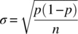
In this case study, the bit‐error performance of a BPSK‐modulated waveform is evaluated using a Monte Carlo simulation. The emphasis in this case study is on the accuracy of the simulation in predicting the known theoretical performance given by

The error in the evaluation of Pbe is measured as the percentage error relative to the theoretical value given a fixed number of Monte Carlo trials for each signal‐to‐noise ratio. Furthermore, because the Q‐function describes the theoretical performance under ideal conditions of frequency, phase and bit timing, these results are based on the conditions: fd = ![]() = 0 and φo = 0. In addition, the simulation models the optimally sampled matched filter output so the exact symbol timing is known. With these ideal conditions, including the AWGN channel, it is convenient to use only one sample‐per‐symbol, that is, by letting Ns = 1 the simulation will run considerably faster and the performance will be identical to that for Ns > 1. Based on these conditions, the bit‐error performance of the BPSK received signal plus noise is evaluated using n = 1000 bits or Monte Carlo trials for each signal‐to‐noise ratio. To examine the spread in the bit‐error estimates the simulation is repeated 20 times using different noise generator seeds and the results are plotted in Figure 14.21. From the discussion in Section 14.2.1, the standard deviation in the estimation of Pbe is given by
= 0 and φo = 0. In addition, the simulation models the optimally sampled matched filter output so the exact symbol timing is known. With these ideal conditions, including the AWGN channel, it is convenient to use only one sample‐per‐symbol, that is, by letting Ns = 1 the simulation will run considerably faster and the performance will be identical to that for Ns > 1. Based on these conditions, the bit‐error performance of the BPSK received signal plus noise is evaluated using n = 1000 bits or Monte Carlo trials for each signal‐to‐noise ratio. To examine the spread in the bit‐error estimates the simulation is repeated 20 times using different noise generator seeds and the results are plotted in Figure 14.21. From the discussion in Section 14.2.1, the standard deviation in the estimation of Pbe is given by

and the error‐bars, shown for signal‐to‐noise ratios of Eb/No = 2, 4, 6, and 8 dB, reflect this 1‐sigma range. In this case, σ is the accuracy of the test and the error‐bars are computed as

FIGURE 14.21 Fixed‐length Monte Carlo simulation of BPSK performance in AWGN channel (n = 1 K bits for each signal‐to‐noise ratio with 20 independent repetitions).
With the exception of the 8 dB case, this corresponds to a test confidence of 68.26%, that is, 68.26% of the simulations at the corresponding signal‐to‐noise ratio will fall within error‐bars corresponding to (14.90). The 8 dB case is unique, in that, the lower error‐bar is negative so any estimate less than the upper error‐bar will pass the test; this is referred to as a one‐sided test for which the confidence (Po) is evaluated using (14.8) yielding a confidence of 84.13% as indicated in Table 14.3. Conversion between the confidence of the two‐sided test, involving both upper and lower error‐bars, and the one‐sided test is given by (14.17).
TABLE 14.3 Monte Carlo Simulation Results for Confidence Testing (n = 1000 Samples/MC Simulation, 20 Independent Simulations)
| Eb/No (dB) | Expected Pbe | 1‐Sigma Error | Estimates Within Error Bars | Confidence of Test (%) | Theoretical Confidence (%) |
| 2 | 3.75(−2) | 6.01(−3) | 13 | 65 | 68.26 |
| 4 | 1.25(−2) | 3.51(−3) | 14 | 70 | 68.26 |
| 6 | 2.3883(−3) | 1.55(−3) | 15 | 75 | 68.26 |
| 8 | 1.9091(−4) | 4.37(−4) | 18 | 90 | 84.13a |
a Based on one‐sided error bar.
Table 14.3 summarizes the confidence testing results from Figure 14.21 and compares the results with the theoretical values discussed in Section 14.2.1. For a given Eb/No, the theoretical accuracy in the measurement of Pbe is determined by the confidence level of the test; however, the accuracy can be improved by averaging the number of error in repeated trails at each Eb/No. Normally, it is desired to achieve the accuracy in the simulations at the lowest error probability of interest, for example, by requiring an accuracy of 5% (η = 0.05) at p = Pbe = 10−5 with a 90% confidence level. Under these conditions the accuracy of the test is 0.05 and, from Figure 14.4, ko = 1.3 and using (14.19) the number of Monte Carlo for each signal‐to‐noise ratio is computed as n = 67.6 M bits.
Typically, a simulation is executed to evaluate the performance over a range of signal‐to‐noise ratios. However, it is time‐consuming and often unnecessary to evaluate the performance at the lower signal‐to‐noise ratios with the same number of Monte Carlo trials required to achieve a given accuracy at the higher signal‐to‐noise ratios. For example, when using a 67.6 M‐bit Monte Carlo simulation the average number of errors at Pbe = 10−5 is 676 and the average number of errors at Pbe = 10−2 is 676 K with a commensurate increase in the estimation accuracy and confidence. However, the same measurement accuracy and confidence corresponding to the 10−5 simulation is achieved using a Monte Carlo simulation with only 67.6 K bits at Pbe = 10−2. Therefore, to preserve the same accuracy and confidence for all signal‐to‐noise ratios the simulation can be terminated when a fixed number of errors have occurred for each signal‐to‐noise ratio. This fixed‐error criterion is determined using Figure 14.3 or from (14.20) with p = Pbe and is approximated as

Figure 14.22 shows the simulated bit‐error performance using a fixed number of bit errors e = 676 corresponding to the above example. Two‐sided error‐bars are shown for signal‐to‐noise ratios of 2, 4, 6, 8, and 10 dB and are evaluated using as P = Pbe ± koσ = Pbe (1 ± η) and, while the results of only one Monte Carlo simulation is shown, it is claimed that 90% of the simulated bit‐error results will fall within the error‐bars. The 5% accuracy corresponds to η = 0.05 and, from the performance results in Figure 14.22, the simulation results are seen to accurately represent the theoretical performance.
FIGURE 14.22 Fixed‐error Monte Carlo simulation of BPSK performance in AWGN channel (n = 67.6 M bits for each signal‐to‐noise ratio).
The normalized cumulative central processing unit (CPU) time is summarized in Figure 14.23 for the fixed‐error and fixed‐length criteria using the above example parameters with n = 67.6 M bits for each signal‐to‐noise ratio. The normalization is based on the average of the fixed‐length simulation time for each signal‐to‐noise, denoted Tavg(SNR). The saving in the simulation time for Eb/No = 0 through 10 dB in 1 dB steps when using the fixed‐error criterion is about 4000:1.15

FIGURE 14.23 Monte Carlo simulation cumulative CPU time (fixed‐length = 67.6 M bits, fixed‐error = 676 bits).
14.7 SYSTEM PERFORMANCE EVALUATION USING QUADRATURE INTEGRATION
The Monte Carlo approach to communication system performance simulation discussed in the previous sections can be applied to evaluate algorithms involving quantization, coding, tracking, and the modeling of real‐world channels. However, Monte Carlo simulations are generally time‐consuming especially if accurate results are required at very low error probabilities. Evaluation of the demodulator detection error probability necessarily involves performing intricate integrations defined over a range of the integration variable. An alternative approach to the performance evaluation involves using numerical analysis techniques referred to as quadrature integration. Although limited to specific applications, these numerical techniques provide rapid and accurate assessments of the system performance and are useful in characterizing the performance sensitivities to various anomalies in the early state of the waveform selection and system design process. The numerical analysis technique of interest involves the approximate evaluation of integrals using quadrature integration [28].
The term quadrature integration results from the underlying quadrature polynomials used in the approximate evaluation of integrals of the form

where w(x) is a weighting function satisfying the integral equation

In (14.93) ![]() represents a set of orthogonal polynomials over the interval (a,b) with respect to the weighting function w(x). The values xi correspond to the zeros of the polynomial Φi(x) and the coefficients Ai are weights determined as
represents a set of orthogonal polynomials over the interval (a,b) with respect to the weighting function w(x). The values xi correspond to the zeros of the polynomial Φi(x) and the coefficients Ai are weights determined as

where

The polynomials associated with various weighting functions are identified in Table 14.4.
TABLE 14.4 Summary of Some Orthogonal Polynomials for Quadrature Integration (Page Numbers Refer to Reference 28)
| Polynomial | Φi(x) | w(x) | ki | (a,b) |
| Legendre (Gaussian), p. 26 |  |
1 | (−1,1) | |
| Chebyshev (first kind), p. 27 |  |
 |
(−1,1) | |
| Chebyshev (second kind), p. 29 |  |
π/2 | (−1,1) | |
| Chebyshev–Hermite, p. 33 | (−∞,−∞) | |||
| Chebyshev–Laguerrea, p. 34 | (0,−∞) |
a For x ≥ 0.
These relationships are developed by Krylov [28] including the characterization of the error in the approximation of (14.92) and tables of abscissa xi and coefficient values Ai for the various quadrature integration approximations. The Legendre polynomial results in Gauss‐quadrature integration with w(x) = 1. In general, the integration limits are finite with range (a,b). However, by changing the integration variable to correspond to the range (−1, 1) the coefficients Ai are symmetrical in ± xi as provided in most of tabulations. The values of xi and Ai for the Chebyshev polynomials of the first kind are easily calculated as

where the coefficients Ai are constant, independent of i. The topic of orthogonal polynomials is also discussed in Chapter 22 of Abramowitz and Stegun [5] with extensive tables of xi and Ai provided in Chapter 25. The tabulated data are usually given with 15–20 decimal places so the numerical evaluation should be used with a commensurate degree of precision. The abscissas and weight values for the Hermite integration used in the following case studies are listed in Table 14.5.
TABLE 14.5 Abscissas and Weights for Hermite Integrationa (Symmetrical Weightsb for N = 20)c
| n | Abscissa (±xi) | Weights (wi) |
| 1 | 0.24534 07083 009 | 4.62243 66960 06 (−1) |
| 2 | 0.73747 37285 454 | 2.86675 50536 28 (−1) |
| 3 | 1.23407 62153 953 | 1.09017 20602 00 (−1) |
| 4 | 1.73853 77121 166 | 2.48105 20887 46 (−2) |
| 5 | 2.25497 40020 893 | 3.24377 33422 38 (−3) |
| 6 | 2.78880 60584 281 | 2.28338 63601 63 (−4) |
| 7 | 3.34785 45673 832 | 7.80255 64785 32 (−6) |
| 8 | 3.94476 40401 156 | 1.08606 93707 69 (−7) |
| 9 | 4.60368 24495 507 | 4.39934 09922 73 (−10) |
| 10 | 5.38748 08900 112 | 2.22939 36455 34 (−13) |
a Also referred to as Chebyshev–Hermite polynomial.
b Attributed to Salzer, Zucker, and Capuano [30].
c Abramowitz [29]. Courtesy of U.S. Department of Commerce.
14.8 CASE STUDY: BPSK BIT‐ERROR EVALUATION WITH PLL TRACKING
Based on the signal‐to‐noise ratio, the bit‐error probability of the BPSK‐modulated waveform, conditioned on a phase error, is given by
where γb = Eb/No is the signal‐to‐noise ratio in the bandwidth equal to the bit rate Rb. The bit‐error probability is then evaluated by removing the conditioning based on the pdf of the random phase resulting in

where the range of integration is ![]() . The random phase function at the output of a second‐order phaselock loop is characterized by the Tikhonov [31] pdf expressed as
. The random phase function at the output of a second‐order phaselock loop is characterized by the Tikhonov [31] pdf expressed as

where ![]() is the phase variance and Io(x) is the zero‐order modified Bessel function of the first kind. Viterbi [32] also derives (14.99) and discusses its applicability to the second‐order phaselock loop. The phase variance
is the phase variance and Io(x) is the zero‐order modified Bessel function of the first kind. Viterbi [32] also derives (14.99) and discusses its applicability to the second‐order phaselock loop. The phase variance ![]() is related to the signal‐to‐noise ratio γL, measured in the phaselock loop bandwidth and the squaring loss SL by the expression
is related to the signal‐to‐noise ratio γL, measured in the phaselock loop bandwidth and the squaring loss SL by the expression
The signal‐to‐noise ratio in the loop bandwidth is computed as

where BL is the phaselock loop bandwidth and Bb is the bandwidth corresponding to the bit‐rate Rb of the BPSK‐modulated waveform; the ratio BL/Bb is generally expressed as the time‐bandwidth product (BLT) of the loop where T = 1/Rb for BPSK. The squaring loss of the phaselock loop is associated with the removal of the biphase data modulation. The phase distribution, expressed by (14.99), is based on a continuous wave (CW) received signal with AWGN and a second‐order phaselock loop. However, inclusion of the squaring loss in evaluating the phase variance, as in (14.100), accounts for the loss associated with the binary data modulation. The squaring loss for BPSK modulation is discussed in Chapter 10 and, for matched filter detection, is expressed as
14.8.1 BPSK Bit‐Error Evaluation Using Tikhonov Phase Distribution
Substitution of (14.97) and (14.99) into (14.98) with ![]() results in the bit‐error expression
results in the bit‐error expression

This result can be put into the quadrature integration form, using the Chebyshev polynomial of the first‐kind, through the variable substitution x = ϕ/π with dϕ = π dx. The resulting expression is

where
The constants Ai and xi are evaluated using (14.96) with xi evaluated over the range − N′ ≤ i ≤ N′, where N′ = (N − 1)/2 for N = odd integer and N′ = N/2 for N = even integer.
14.8.2 BPSK Bit‐Error Evaluation Using Gaussian Phase Approximation
The Tikhonov phase pdf approaches a Gaussian distribution as the input signal‐to‐noise increases resulting in
Using (14.106) and (14.97) with (14.98), the quadrature integration using the Chebyshev–Hermite polynomial results in the following expression for the bit‐error probability

where
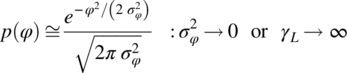
The first approximation results because the range of p(φ) is (−π,π) and the integration limits are (−∞,∞); this assumes that p(φ) is essentially zero outside of the range (−π,π) which is valid as ![]() .
.
Using (14.108), Equation (14.107) is evaluated for N = 2016 abscissa and weight values for Hermite integration are listed in Table 14.5 and the results are plotted in Figure 14.24 as the solid lines for BLT = 0.5 and 0.1. The dotted line represents the theoretical performance of antipodal signaling and the circled data points are evaluated using (14.107) with σφ = 0, independent of the signal‐to‐noise ratio. The circled data points are a special case used to examine the performance of antipodal signaling using quadrature integration and it is seen from the figure that the results are identical.

FIGURE 14.24 Performance of BPSK using Chebyshev–Hermite quadrature integration (Gaussian phase approximation).
14.9 CASE STUDY: QPSK BIT‐ERROR EVALUATION WITH PLL TRACKING
Based on the signal‐to‐noise ratio out of each baseband channel, the symbol‐error probability conditioned on the phase error for QPSK modulation is given by

The symbol‐error probability is evaluated by removing the conditioning as expressed by (14.98), substituting Pse for the QPSK waveform in place of Pbe, and using either the Tikhonov phase pdf for QPSK expressed as

or the high signal‐to‐noise ratio Gaussian approximation of (14.106).
14.9.1 QPSK Bit‐Error Evaluation Using Tikhonov Phase Distribution
In this case quadrature integration using the QPSK Tikhonov’s phase pdf is performed using Legendre polynomials with weight w(x) = 1.0 and integration limits (−1,1). Upon making the substitution of variable ![]() this approach results in Gaussian integration, using the Legendre polynomial, expressed as
this approach results in Gaussian integration, using the Legendre polynomial, expressed as

where
and

In evaluating these integrals, or summations, the phase variance for the QPSK phaselock loop is given by
where γL is the signal‐to‐noise ratio in the loop bandwidth, BL, and SL4 is the squaring loss resulting from the processing required to remove the quadrature phase modulation for the carrier recovery. For QPSK, the signal‐to‐noise ratio in the loop bandwidth is expressed as
where Es is the symbol energy and T is the symbol duration. The squaring loss for QPSK is discussed in Chapter 10.
The abscissa and coefficient values are tabulated [33] for N = 2 through 96 corresponding to symmetrical summations on xi from −N/2 ≤ i ≤ N/2 for N = even integer and −(N − 1)/2 ≤ i ≤ (N − 1)/2 for N = odd integer.
14.9.2 QPSK Bit‐Error Evaluation Using Gaussian Phase Approximation
With this approximation the integral for the QPSK symbol error is approximated using the Chebyshev–Hermite polynomial integration as in Section 14.8.2. For this evaluation, let ![]() and evaluate the integral as
and evaluate the integral as

where
The standard deviation of the phase is evaluated from (14.115) using the signal‐to‐noise ratio in the phaselock loop bandwidth γL and the squaring loss SL4 as discussed in the preceding section. The abscissa and coefficient values for the Chebyshev–Hermite polynomial integration are tabulated [32] for N = 2–20.
ACRONYMS
- AR
- Autoregressive (model)
- AWGN
- Additive white Gaussian noise
- BPSK
- Binary phase shift keying
- CPU
- Central processing unit (computer)
- CW
- Continuous wave
- DSP
- Digital signal processing (processor)
- FEC
- Forward error correction
- IF
- Intermediate frequency
- ISI
- Intersymbol interference
- LR
- Likelihood ratio
- LLR
- Log‐likelihood ratio
- OQPSK
- Offset quadrature phase shift keying
- PN
- Pseudo‐noise
- PSD
- Power spectral density
- QPSK
- Quadrature phase shift keying
- RF
- Radio frequency
PROBLEMS
- Show that Equation (14.15) leads to (14.16) under the conditions
 and
and  .
. - Derive equation (14.17).
- For a correct‐acceptance criteria of 95%, the single‐threshold Poisson test results in an accuracy of 40% with npo = 80. Determine the npo product for the single‐threshold Gaussian test under the same conditions, that is, a test confidence of 95% and accuracy of 40%. Assuming a bit‐error probability test with a bit‐rate of 75 bits‐per‐second and po = 10−3, what is the test time in minutes for each test?
- Derive the optimum single‐threshold for deciding between hypothesis H0 and H1 using the binomial distribution.
- Using the binomial coefficient nCk, derive the recursive relationship for
 .
. - Using the binomial density function p(k), derive the recursive relationship for p(k + 1).
- Design a sequential sampling test involving the flipping of a coin that is known to be either balanced with a probability of heads of p0 = 0.5 under hypothesis H0 or unbalance with a probability of heads of p1 = 0.7 under hypothesis H1. The coin is to be tested with a confidence level of 95% and a significance level of 5% under H0. To complete this problem fill out Table 14.1 with the test requirements and parameters for this test.
- For the test designed in Problem 7, sketch the test boundaries as in Figure 7 and flip a coin a number of times, indexing k by one if a tail appears and plotting the results on the sketch.
- Express the mean value of the uniform distribution shown in Figure 14.13 in terms of the probability 0 ≤ p ≤ 1 and q = 1 − p.
- Plot or sketch the binomial distribution for a sequence of length 4 using the Bernoulli random number generator with p = 0.2, 0.5, and 0.8.
- Write a computer code to implement the congruence method for generating uniformly distributed random numbers given by (14.45) using A = 9, B = 25853, and C = 32768. Replace the coin flipping example in Problem 10 with your random number generator code with binary 1 = heads and −1 = tails and repeat the sequential test procedure as outlined in Problem 10 under the following conditions:
- Using a balanced binary generator.
- Using an unbalanced binary generator with Pr (tails) = 0.6.
- Applying the convolution integral to the uniform probability density function of Figure 14.1 with a = −1 and b = 1, form the pdf of the sum of three uniformly distributed probability random variables. Plot the resulting distribution and compare it with the Gaussian distribution with variance
 where
where  is the variance of the uniform distribution.
 - Using the uniform random number generator code in Problem 11 with p = 1/2, form the summationfor j = 1,1000 and plot a histogram of the occurrences of Yj ranging in amplitude from −3 to 3 in steps of 0.1. Compare the resulting histogram plot with the distributions in Problem 11.

- Using the uniform random number generator code in Problem 11 generate simulated Poisson random variables for k = 3 and 0 ≤ τ ≤ 10 and plot the resulting pdf. To plot the pdf use a histogram with 101 bins (including the τ = 0 bin), a bins size corresponding to τ/10 and a sample size of 10,000 trials. Compare the simulated pdf with the corresponding theoretical pdf shown in Figure 11.
- Referring to the (14.74) and (14.75) express the magnitude and phase functions in (14.77) and (14.78)respectively in terms of the MSK‐modulated waveform with
 and
and  . Noting that fmT = 1/2, dci = rect((t − iT)/T), and dsi = rect((t − T/2 − iT)/T) evaluate and plot the phase function for dci,dsi =
  , that is, the dci and dsi correspond, respectively, to constant mark and space data.
 - Evaluate the carrier power Ps given by (14.79) for QPSK modulation waveform using the real signal s(t) and the analytic signal
 . Repeat this evaluation for the MSK‐modulated waveform. In each case, state the relationship between the true or actual signal power based on the real signal and that corresponding to the analytic signal.
 - Referring to the discussion following (14.87) consider a simulation program that implements a transmitted signal with independent inphase and quadrature data modulation functions mc(iTs) and ms(iTs) with Ns samples‐per‐symbol and a sampling interval of Ts seconds. The transmitted signal is implemented aswhere V is the peak voltage of an equivalent modulated carrier frequency. The signal is passed through an AWGN channel and the resulting received signal is
 where nc(iTs) and ns(iTs) are iid Gaussian random variables characterized by N(0,σn) where the noise standard deviation is computed as
 where γs = γb/Ns = 10γb(dB)/10/Ns. The corresponding carrier modulated power is
  and the noise power and signal‐to‐noise ratio in the bandwidth equal to bit rate Rb are
  and γb respectively. Considering that mc(t) = dc rectT(t − T/2 − mT) and ms(t) = ds rectT(t − T/2 − mT) with dc,ds = {±1}, determine the signal and noise powers and the signal‐to‐noise ratio at the output of the demodulator matched filter.
Replace V with
 and the Gaussian noise N(0,σn) with
  and repeat this problem.
 - Given the Gaussian random variable x described by N(0,σ), set‐up the problem to evaluate the mean value of g(x) using quadrature integration whereIdentify the underlying orthogonal polynomial. Hint: The mean value of g(x) is evaluated as


- Using the Tikhonov phase pdf for BPSK and (14.105), evaluate (14.104) and plot the bit‐error probability versus γb using the Chebyshev polynomial of the first‐kind using coefficients Ai and zeros xi given by (14.96). Note: The results should compare favorably with Figure 14.24.
- Show that the Tikhonov phase pdf given by (14.99) is approximated by the zero mean Gaussian pdf of (14.106) as the phase variance
 approaches zero.
 - Derive (14.108) for the evaluation of Pbe with BPSK modulation given by (14.107) using Gaussian approximation to the Tikhonov phase pdf.
- Evaluate the bit‐error probability for QPSK modulation using the Gaussian approximation to the Tikhonov phase pdf.
REFERENCES
- 1. K.S. Shanmugam, P. Balaban, “A Modified Monte Carlo Simulation Technique for the Evaluation of Error Rate in Digital Communication Systems,” IEEE Transactions on Communications, Vol. COM‐28, No. 11, pp. 1916–1924, November 1980.
- 2. A. Papoulis, Probability, Random Variables, and Stochastic Processes, p. 57, McGraw–Hill, New York, 1965.
- 3. W. Feller, An Introduction to Probability Theory and Its Applications, John Wiley & Sons, Inc., New York, 1957.
- 4. A. Papoulis, Probability, Random Variables, and Stochastic Processes, p. 69, McGraw–Hill, New York, 1965.
- 5. M. Abramowitz, I.A. Stegun, Editors, Handbook of Mathematical Functions with Formulas, Graphs, and Mathematical Tables, Applied Mathematics Series No. 55, National Bureau of Standards, Washington, DC, June 1964.
- 6. A. Papoulis, Probability, Random Variables, and Stochastic Processes, pp. 966–973, McGraw–Hill, New York, 1965.
- 7. A. Papoulis, Probability, Random Variables, and Stochastic Processes, pp. 71–73, McGraw–Hill, New York, 1965.
- 8. W.B. Davenport, Jr., W.L. Root, An Introduction to the Theory of Random Signals and Noise, Chapter 14, McGraw–Hill, New York, 1958.
- 9. H.D. Brunk, An Introduction to Mathematical Statistics, Blaisdell Publishing Company, Waltham, MA, 1965.
- 10. A. Wald, Statistical Decision Functions, John Wiley & Sons, Inc., New York, 1950.
- 11. H.D. Brunk, An Introduction to Mathematical Statistics, Chapter 16, “Other Sampling Methods,” Blaisdell Publishing Company, Waltham, MA, 1965.
- 12. A. Wald, Sequential Analysis, John Wiley & Sons, Inc., New York, 1947.
- 13. M. Abramowitz, I.A. Stegun, Editors, Handbook of Mathematical Function with Formulas, Graphs, and Mathematical Tables, pp. 949–953, Applied Mathematics Series No. 55, National Bureau of Standards, Washington, DC, June 1964.
- 14. H.A. Meyer, Symposium on Monte Carlo Methods, John Wiley & Sons, Inc., New York, 1956.
- 15. A.O. Arthur, Random Digit Generation, Computing News, September 1956.
- 16. R.P. Chambers, “Random‐Number Generation on Digital Computers,” IEEE Spectrum, Vol. 4, pp. 48–56, February 1967.
- 17. D.E. Knuth, The Art of Computer Programming, Volume 2: Semi‐Numerical Algorithms, pp. 170–173, Addison‐Wesley, Reading, MA, 1981.
- 18. M.E. Muller, “An Inverse Method for the Generation of Random Normal Deviates on Large‐Scale Computers,” Mathematical Tables and Other Aids to Computation, Vol. 63, pp. 167–174, 1958.
- 19. C. Hastings, Jr., Approximations for Digital Computers, Princeton University Press, Princeton, NJ, 1955
- 20. M. Abramowitz, I.A. Stegun, Editors, Handbook of Mathematical Function with Formulas, Graphs, and Mathematical Tables, p. 933, Applied Mathematics Series No. 55, National Bureau of Standards, Washington, DC, June 1964. (Also includes many other approximations by C. Hastings, Jr.).
- 21. A. Papoulis, Probability, Random Variables, and Stochastic Processes, pp. 266–268, McGraw–Hill, New York, 1965.
- 22. E. Parzen, Modern Probability Theory and Its Applications, John Wiley & Sons, Inc., New York, 1960.
- 23. A. Papoulis, Probability, Random Variables, and Stochastic Processes, pp. 220–221, McGraw–Hill, New York, 1965.
- 24. S. Haykin, Adaptive Filter Theory, pp. 67–85, Prentice‐Hall, Englewood, NJ, 1986.
- 25. W.C. Jakes, Microwave Mobile Communications, John Wiley & Sons, Inc., New York, 1975.
- 26. L. Kleinrock, Queueing Systems, Volume 1: Theory, John Wiley & Sons, Inc., New York, 1975.
- 27. A. Papoulis, Probability, Random Variables, and Stochastic Processes, pp. 556–560, McGraw–Hill, New York, 1965.
- 28. V.K. Krylov, Approximate Calculation of Integrals, Translated by A.H. Stroud, The Macmillan Company, New York, 1962.
- 29. M. Abramowitz, I.A. Stegun, Editors, Handbook of Mathematical Function with Formulas, Graphs, and Mathematical Tables, p. 924, Applied Mathematics Series No. 55, National Bureau of Standards, Washington, DC, June 1964.
- 30. M. Abramowitz, I.A. Stegun, Editors, Handbook of Mathematical Functions with Formulas, Graphs, and Mathematical Tables, Chapter 25, “Table of the Zeros and Weight Factors of the First Twenty Hermite Polynomials,” p. 924, Applied Mathematics Series No. 55, National Bureau of Standards, Washington, DC, June 1964.
- 31. W.C. Lindsey, M.K. Simon, Telecommunication Systems Engineering, Dover Publications, Inc., New York, 1973.
- 32. A.J. Viterbi, Principles of Coherent Communication, pp. 86–96, McGraw–Hill, New York, 1966.
- 33. M. Abramowitz, I.A. Stegun, Editors, Handbook of Mathematical Function with Formulas, Graphs, and Mathematical Tables, Applied Mathematics Series No. 55, National Bureau of Standards, Washington, DC, pp. 916–919, June 1964.