
19
ATMOSPHERIC PROPAGATION
19.1 INTRODUCTION
Communication links that propagate through the atmosphere encounter a number of effects that distort the received signal making detection and parameter estimation difficult and prone to errors. The signal distortion results because the atmosphere is an inhomogeneous medium with spatial and temporal variations that result in random behavior leading to: absorption or signal attenuation, inter‐ and intra‐symbol distortion due to symbol dispersion, variations in range‐delay, Doppler spreading, polarization rotation, and signal amplitude and phase fluctuations resulting from multipath interference. The principal regions of the atmosphere that impact electromagnetic wave propagation are the troposphere, and ionosphere, and the principal parameter that characterizes the performance in each region is the index of refraction.
The lower region of the atmosphere is the troposphere extending to about 30 km in altitude and the upper region is the ionosphere extending to several thousand kilometers. The troposphere is essentially an ion‐free region consisting of about 99% oxygen with nitrogen and water vapor at the lower altitudes. In this region electromagnetic wave propagation characteristics are determined by the refractive index which is a function of pressure, temperature, and water vapor; other natural phenomena like dust, rain, and clouds must also be considered. Propagation in the ionosphere is influenced primarily by free‐electrons and characterized by the electron content, the Earth’s magnetic field, and diurnal variations influenced by the Sun. Variations in the atmosphere are influenced by location, season, weather, and the time‐of‐day (TOD). Typically, the mean and stand deviation of the influential parameters are given for a specified season and location.
The impact of these natural occurrences in the atmosphere on the communication signal is dependent upon the carrier frequency and bandwidth of the communication link as well as the antenna beamwidth, height, and the elevation angle of the encounter. The various phenomena resulting from the encounter with the atmospheric channel are characterized in terms of the operating modes as shown in Figure 19.1. The effective Earth radius re is chosen to be (4/3)Re, where Re = 6371 km is the average Earth radius. This selection of re provides for line of sight (LOS) radio frequency coverage to locations that would otherwise be over‐the‐horizon. This LOS condition applies for altitudes less than about 4 km and is discussed in more detail in the following section. The factor of 4/3 is computationally convenient because it is based on a linearly decreasing index of refraction with height, whereas, an exponentially decreasing function with height is in more agreement with in situ measurements and is discussed in Section 19.5.

FIGURE 19.1 Various propagation modes depending on atmospheric conditions, frequency, and geometry.
In Section 19.3, the impact of multipath reflections from a smooth Earth is examined followed by a case study in Section 19.4. Signal refraction in the troposphere and ionosphere is discussed in Section 19.5 and diffraction from irregular surfaces is discussed in Section 19.6 with examples of irregular terrain and urban propagation losses given in Sections 19.7 and 19.8.
19.2 COMMUNICATION LINK GEOMETRY FOR CURVED EARTH
The geometry for determining the propagation paths for LOS and multipath rays has been modeled under various simplifying assumptions involving a flat‐Earth approximation and a spherical Earth with receivers at sufficiently long ranges such that the direct and reflected waves are assumed to be parallel. Although there is no known exact solution to the general case involving unrestricted ranges, transmitter, and receiver heights, Fishback [1] provides a solution involving a spherical Earth model, with effective Earth radius re to account for refraction and unrestricted transmitter and receiver heights. Fishback’s analysis assumes the transmitter and receiver heights, h1 and h2, are given along with the length of the ground range, G, between the two points. Fishback’s solution is somewhat restricted by assuming small grazing angles. Instead of following Fishback’s solution, the relationships developed by Blake [2] are discussed because they are less prone to numerical and computational inaccuracies due to rounding and because Blake’s solution simply requires the specification of h1, h2 and the LOS range, Rd, between the transmit and receive points and there is no restriction on the grazing angle. The geometry of the encounter is shown in Figure 19.2.

FIGURE 19.2 Spherical‐earth encounter geometry.
The following analysis outlines the procedures for the solution of the reflected wave at the receiver terminal in terms of R1, R2, and ψ. With these parameters, the amplitude and delay of the interfering signal can be determined relative to the LOS signal. To begin, the angle θd is computed as

As shown in Figure 19.2 the angle θd corresponds to a negative angle, that is, when the transmitter is looking below the local horizon. The approximation in (19.1) applies when h1, h2 ≪ re. The ground path, as derived by Blake, is determined using the direct path length Rd and is computed as

The ground range G is defined as G = G1 + G2 and Fishback has shown that G1 is the solution to a cubic equation involving G, h1, h2, and re. When h1, h2 ≪ re, the solution is

where

and

The angles ϕ1 and ϕ2 are then determined as
and
from which the ranges R1 and R2 are determined as

and

Using the range R1, the depression angle of the reflected wave is determined as

and the grazing angle is determined as

Referring to Figure 19.2, the grazing angle is also expressed as ![]() . The approximations in (19.10) and (19.11) apply when h1, h2 ≪ re. Using these relationships, the difference between the direct path Rd and the reflected path R1 + R2 is determined as
. The approximations in (19.10) and (19.11) apply when h1, h2 ≪ re. Using these relationships, the difference between the direct path Rd and the reflected path R1 + R2 is determined as

The second of these solutions [3] is preferred because it is not subject to numerical errors encountered when performing the subtraction in the first solution. Referring to Figure 19.1, the LOS criterion corresponds to a zero degree grazing angle or the equivalent requirement that Rd = R1 + R2. Therefore, using (19.11), the LOS criterion, involving h1 and h2, is evaluated as

Therefore, when Rd > R the LOS path will exhibit ground reflections, otherwise, the over‐the‐horizon reception occurs from diffraction or refraction as depicted in Figure 19.1.
Although the analysis of the geometry in this section is correct for Rd ≤ R1 + R2, the application to multipath interference based on reflections strictly applies for LOS paths a few degrees above the radio horizon such that δR ≫ λ/4. For lower elevation angles, θd, an intermediate region is entered between the reflection and diffraction regions. When the Earth is modeled with a smooth surface, the region below the radio LOS, shown as the heavy dashed lines in Figure 19.1, is the diffraction region; however, the intermediate region just above and below the radio LOS requires special consideration as described by Fishback. Fishback’s solution is outlined by Blake [4] for the first diffraction mode, that is, when δR ≤ λ/4 and the solution of Burroughs and Atwood [5] is outlined by Barton [6]. In the following section, the impact of reflections from a smooth Earth is examined followed by a case study in Section 19.4 involving a low Earth orbit satellite.
19.3 REFLECTION
Electromagnetic wave propagation is characterized by Huygens’ principle [7] which states that points along the wavefront depicted in Figure 19.3 behave like secondary sources of wavelets that spread out in all directions with velocities that are functions of the propagation medium. This principle provides for the analysis of wave reflection when the wavefront is incident to a reflecting surface. It also provided for the analysis of refractive wave bending and propagation beyond LOS conditions as discussed in Section 19.5.

FIGURE 19.3 Huygens’ principle for advancing wavefront.
Consider the incident wave shown in Figure 19.4 having uniform phase along the wavefront represented by the straight line intersecting the reflecting surface with an angle‐of‐incidence ϕ1. The incident wave is traveling in the medium above the reflecting surface at a velocity ![]() , where u and ε are the permeability and permittivity of the medium. The angle ϕ2 of the reflected wave is determined using Huygens’ principle recognizing that the velocity of the reflected wave is also equal to v. For example, when a wavelet of the incident wave travels the distanced d = vt and intersects the surface, the reflected wave t seconds earlier has traveled the same distance describing the reflected wavefront at the angle of reflection ϕ2. Upon application of elementary geometry, it is found that the angle of reflection is equal to the angle of incidence, that is, ϕ2 = ϕ1. In many practical applications, the reflecting surface is not an ideal reflector and wave refraction occurs resulting in the incident wave propagating through the surface into the second medium with different electromagnetic properties; wave refraction is discussed in Section 19.5. In general, both wave reflection and refraction occur at the surface between two different medium.
, where u and ε are the permeability and permittivity of the medium. The angle ϕ2 of the reflected wave is determined using Huygens’ principle recognizing that the velocity of the reflected wave is also equal to v. For example, when a wavelet of the incident wave travels the distanced d = vt and intersects the surface, the reflected wave t seconds earlier has traveled the same distance describing the reflected wavefront at the angle of reflection ϕ2. Upon application of elementary geometry, it is found that the angle of reflection is equal to the angle of incidence, that is, ϕ2 = ϕ1. In many practical applications, the reflecting surface is not an ideal reflector and wave refraction occurs resulting in the incident wave propagating through the surface into the second medium with different electromagnetic properties; wave refraction is discussed in Section 19.5. In general, both wave reflection and refraction occur at the surface between two different medium.

FIGURE 19.4 Wave reflection from a surface (application of Huygens’ principle yields: ϕ2 = ϕ1).
19.3.1 Reflection from Earth’s Surface
Signal reflection occurs when an incident electrometric wave intersects a large surface with dimensions much greater than the carrier wavelength. In long‐distance communication links, signal reflections from the Earth’s surface will combine with a direct path signal resulting in received signal variations referred to as multipath fading. On a smaller scale, signals in a mobile communication system will reflect off of building and other structures often without an identifiable direct signal path. In these situations, the received signal will fluctuate rapidly with the dynamics of the mobile unit. Signal reflections are characterized in terms of the complex reflection coefficient
where ρ = |Er/Ei| is the magnitude of the reflected‐to‐incident electric field ratio and Φ is the corresponding angle of Er/Ei. The ranges of ρ and Φ are: 0 ≤ ρ ≤ 1 and |Φ| ≤ π and when Φ > 0 then the reflected electric field lags the incident electric field. Ramo and Whinnery [8] provide a detailed discussion of the reflection of electromagnetic wave forming the basis of the following results.
The reflection coefficient also depends on the grazing angle and polarization of the incident electric field and for horizontally and vertically polarized waves the results are expressed as [9]
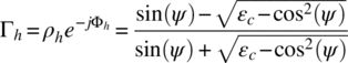
and

where εc is the complex dielectric constant given by
where εr is the ordinary dielectric constant and εi is given by
where λ is the carrier wavelength and σ is surface conductivity.1 When λ is in meters then σ has units of mhos per meter; values of εr and σ for various types of surfaces are given in Table 19.3.
The reflection coefficient for the vertically polarized wave is examined by substituting (19.17) into (19.16) and the resulting amplitude and phase functions are plotted in Figures 19.5 and 19.6 for the indicated conditions. The grazing angle corresponding to the minimum magnitude of the reflection coefficient in Figure 19.5 is referred to as the pseudo‐Brewster angle. With a perfect dielectric, the minimum magnitude of the reflection coefficient is |Γv| = 0, that is, no reflection occurs, and the corresponding grazing angle is referred to as the polarizing angle or, in geometrical optics, the Brewster angle. The Brewster angle occurs only with a vertically polarized wave. With horizontal polarization, the reflection coefficient decreases slowly with grazing angle and the angle Φh is very close to π radians over the entire range of grazing angles.

FIGURE 19.5 Magnitude of reflection coefficient for vertical polarization (conductivity = 0.005 mho/m, dielectric constant = 15).

FIGURE 19.6 Phase of reflection coefficient for vertical polarization (conductivity = 0.005 mho/m, dielectric constant = 15).
Circularly polarized waves are described in terms of horizontally and vertically polarized waves that are in quadrature with one another. Right‐hand circular polarization occurs when the horizontal polarized wave lags that of the vertically polarized wave, that is, when ϕh − ϕv > 0 and left‐hand circular polarization occurs when ϕv − ϕh > 0. For right‐hand or left‐hand circularly polarized incident waves, the reflection coefficient with the same‐sense as the incident wave is expressed as [2, 11]
and the reflection coefficient with the opposite‐sense as the incident wave is
Therefore, in general, both senses of the incident circular polarized wave appear at the receiver from the reflecting surface.
19.4 CASE STUDY: LEO SATELLITE MULTIPATH PROPAGATION
Under ideal conditions, a signal transmitted along a noise‐free direct propagation path is received with a constant signal amplitude and phase. However, with multipath propagation there are one or more signal propagation paths that result from reflections that interfere with the direct path signal causing amplitude and phase fluctuations. This scenario is depicted in Figure 19.7 for a communication link between a ground terminal and a satellite with a single‐point reflection from the Earth’s surface. The description of the various parameters and additional geometrical details regarding this encounter are identified in Figure 19.2.
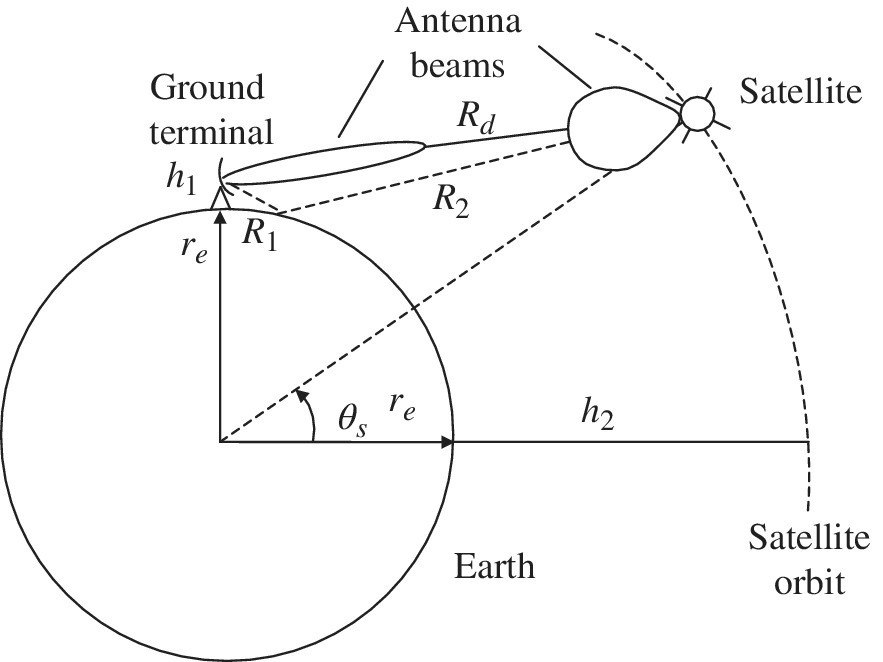
FIGURE 19.7 Communication link with single ray reflection from the Earth’s surface.
The description of the spherical Earth geometry given in Section 19.2 uses the LOS range Rd as the independent variable; however, in this case study, the independent variable is the transmitter elevation angle θd. Using the parameters h1 and h2, the direct path range is computed as a function of θd using the following relationship
The transmitter beam depression angle θbt between the elevation angle and the reflection path R1 is also required to determine the antenna sidelobe level in the direction of the reflection; this angle is simply computed as
A similar angle is required to evaluate the receiver beam depression angle θbr to determine the antenna sidelobe level in the direction of the reflection along the path R2 and, referring to Figure 19.2, this angle is computed as

In the following analysis, the ground and satellite terminal antennas are modeled as uniformly weighted circular aperture antennas as described in Section 15.3.2 with specified gains Gt and Gr respectively. The antenna gains are related to the antenna area Aa or the effective area Ae = naAa, where na is the antenna efficiency, and the gain is computed using (15.61) with the area for the circular aperture antenna given by
where D is the antenna diameter. From Table 15.3, the antenna beamwidth is given by
where λ is the wavelength of the carrier frequency.
Neglecting channel and receiver noise, the signals sd(t) and sr(t) are the received signals at the satellite from the direct and reflected paths respectively. These signals are combined at the receiver to form the received signal s(t) expressed as

where Pt is the transmitted signal power at the antenna input, ωc is the carrier angular frequency, Td, Tr and fd, fr are the delays and propagation factors along the respective paths and Γ is the complex reflection coefficient given by (19.14). Referring to (15.6), the propagation factors are evaluated as

and

The antenna beam angles θbt and θbr are in the direction of the transmitted and reflected waves along the respective paths R1 and R2 and the angles βt and βr are the corresponding antenna‐dependent signal phase along these paths; typically βt and βr are either 0 or π radians depending on the sign of the antenna sidelobes. As depicted in Figure 19.7, ideal beam tracking corresponds to θt, θr = 0. Upon substituting (19.27), (19.28), and (19.14) into (19.26) and factoring out the direct path received signal, the satellite received signal is expressed as

The magnitude of the additive term is evaluated as

In (19.30), the subscript “n” on the antenna gains indicate normalized gains with unit peak gain. The free‐space loss ratio is given by

Also, the carrier frequency phase term is expressed as

This phase term results in large, frequency‐dependent, amplitude fluctuations as the range difference between the direct and reflected wave change. The magnitude of the term in the square brackets in (19.29) is defined as the multipath factor Fm given by

To demonstrate the severity of the multipath on the desired or direct path signal sd(t), the multipath factor is plotted in Figure 19.8 for a satellite in a LEO circular orbit, coplanar with the Earth terminal and using ideal omnidirectional antennas, that is, the gains are assumed to be identical in all directions. In this and the remaining plots, vertical antenna polarization is used, the atmospheric loss along each path is assumed to be identical, that is, Latmr = Latmt and the parameter values listed in Table 19.1 are used.

FIGURE 19.8 Communication link with single‐ray reflection (omnidirectional antennas).
TABLE 19.1 Parameter Values for Multipath Factor (Fm) Evaluation
| Parameter | Value | Comment |
| Re | 6371 | Earth radius (km) |
| re | 8494.66 | 4/3 Earth radius (km) |
| h1 | 30 | Transmitter antenna height (m) |
| h2 | 200 | LEO circular orbita altitude (km) |
| Gt | Variable | Transmit antenna gain |
| Gr | 10 | Receiver antenna gain (dB) |
| ηat | 80 | Transmit antenna efficiency (%) |
| ηar | 80 | Receiver antenna efficiency (%) |
| fc | 500 | Carrier frequency (MHz) |
| σ | 0.005 | Conductivity (mho/m) |
| εr | 15 | Dielectric constant (F/m) |
aCo‐located with the plane of the ground terminal.
Three things are noteworthy in Figure 19.8: the effect of the multipath loss is about the same over all elevation angles θd; the maximum level of the received signal is 6 dB2; the lower limit of received signal is between −42 and −43 dB. The upper and lower limits, corresponding to the solid black curves, result from the constructive and destructive interference of the two received signals based on the phase term in (19.33). When Fm is plotted as a function of the antenna elevation angle, as in Figure 19.8, the phase term varies more slowly at the higher elevation angles where δR changes slowly3; this is evident in Figure 19.7 when θd > 80°.
Figure 19.9 shows the impact of the multipath interference using a transmitter antenna gain of 20 dB; this gain corresponds to a 16.4° antenna beamwidth. The variation in the upper and lower limits of the multipath factor is significantly reduced for elevation angles greater than about 10°. This multipath improvement results from the increasing attenuation of the multipath signal by the antenna sidelobes as the elevation angle increases.

FIGURE 19.9 Communication link with single‐ray reflection (Gt = 20 dB, θBt = 16.2°).
By eliminating the dependence of Fm on the phase function in (19.33), the upper and lower limits on the multipath factor are evaluated as

The squared inverse of the lower limit is defined as the multipath loss and is expressed as
The average multipath loss within the transmitter antenna beamwidth corresponding to a specified θd is denoted as ![]() . Equations (19.34) and (19.35) are used in Chapter 15 to establish the system link loss budget. The multipath loss can be effectively mitigated through the system and waveform designs and demodulator signal processing.
. Equations (19.34) and (19.35) are used in Chapter 15 to establish the system link loss budget. The multipath loss can be effectively mitigated through the system and waveform designs and demodulator signal processing.
Figure 19.10 compares the maximum and minimum multipath factors for transmitter antenna gains of 20, 30, and 40 dB; the 20 dB gain case corresponds to Figure 19.9. The improvements are significant and are accompanied by a lower link power requirement; however, the cost and complexity associated with antenna beam pointing and tracking must be taken into account.

FIGURE 19.10 Communication link with single‐ray reflection from the Earth’s surface (Gt = 20, 30, and 40 dB; θBt = 16.2, 5.2, and 1.64°).
19.5 REFRACTION
Signal refraction occurs when an incident electrometric wave intersects irregularities in the transmission media. Refraction results in electromagnetic wave bending and allows for communications into the shadow region beyond the LOS. For example, wave refraction occurs in regions behind hills, mountains, and other obstructions that are impenetrable by a direct path link. Long‐distance communications experience refraction due to varying dielectric constant in the atmosphere. As in the case of wave reflection, wave bending due to refraction is characterized by Huygens’ principle that is introduced in Section 19.3.
Application of Huygens’ principle together with Snell’s law is used to describe the bending of a plane wave as it propagates through the atmosphere with different refractive indices. This phenomenon is depicted in Figure 19.11 for an abrupt change in the index of refraction. Snell’s law states that when a plane wave propagating in a medium with refractive index n1 intersects a second medium at an angle of incidence ϕ1 with refractive index n2 then the sine of the angle of refraction, ϕ2, is related to the sine of the angle of incidence ϕ1 by the relationship

FIGURE 19.11 Wave bending in the atmosphere (shown for n1 > n2).
The angles ψi, i = 1, 2, are the grazing angles of the plain waves and are related to the incident angles as ψi = π/2 − ϕi radians.
Figure 19.11 is suggestive of uplink propagation with the angle of refraction shown to be greater than the angle of incidence. This corresponds to decreasing electron densities with altitude, that is, n2 < n1, and a bending of the wave that tend to follow the curvature of the Earth giving rise to range delay and angle errors. When the angle of refraction satisfies the condition ϕ2 > π/2 radians, the incident wave is not propagated forward but reflected back through the medium containing the incident wave. Using the angle ϕ2 = π/2 radians, the critical angle of incidence for reflection is determined as

19.5.1 Tropospheric Refraction
Because the troposphere does not contain free‐electrons, signal propagation in the troposphere is influenced principally by water vapor content, air temperature, and pressure. Based on the standard atmosphere described by Kerr [1], the index of refraction in the troposphere is given by

where a and b are constants equal to 79°K/mb and 4800°K respectively; the respective values of a and b as determined by Smith and Weintraub [12] are 77.6°K/mb and 4810°K and by Campen and Cole [13] are 74.4°K/mb and 4973°K. The parameter T is the air temperature in °K, p is the air pressure in millibars (mb) and e is the partial pressure of water vapor in millibars.
Based on the analysis of Campen and Cole as outlined by Millman [14] the parameters describing the standard atmosphere are expressed as a function of altitude or height h in kilometers for h ≤ 10 km as
and
where po = 1013 mb is the standard temperature at sea level and eo is the partial pressure of water vapor at the Earth’s surface in mb. These expressions are essentially independent of frequency. The normalized form, (n − 1)106, of the refractive index is valid to within 0.5% for frequencies below about 30 MHz.
Upon curve fitting these results using a polynomial in h with units of km, Campen and Cole express the refractive index as a function of h through the troposphere for a completely wet environment with 100% relative humidity as

and for a completely dry environment with 0% relative humidity at refractive index is expressed as
Equations (19.42) and (19.43) apply for heights up to 10 km and decay exponentially from 10 km to the upper limit of the troposphere at about 30.5 km according to the relationships
and
These results are plotted in Figure 19.12 in terms of the parameter N = (n − 1)1e6 referred to refractivity.

FIGURE 19.12 Refractive index in troposphere using the standard atmosphere.
Millman uses these results to evaluate the refractive bending along the propagation path using direct integration and ray tracing. In his analysis the troposphere is divided into spherical 30.48 m layers of constant refractive index up to 3.048 km and 3.048 m layers up to 30.48 km; the refractive index above 30.48 km is unity. The refractive bending of the propagation path gives rise to antenna pointing errors, range delay errors, and Doppler frequency errors. An encounter between a ground terminal and an aircraft is depicted in Figure 19.13. The refraction angle and range errors are shown in Figures 19.14 and 19.15 respectively. These errors increase with increasing height and decreasing antenna grazing or apparent elevation angle. For example, with receiver heights above 1853.2 km and zero degree grazing angle the maximum refraction angular errors are 0.799° and 0.049° for the wet and dry conditions respectively. For the wet and dry conditions, the corresponding maximum range errors are about 381 and 290 ft (116 and 88.4 m).

FIGURE 19.13 Tropospheric wave bending encounter. Millman [15].
Reproduced by permission of John Wiley & Sons, Inc.

FIGURE 19.14 Tropospheric refraction angle measurement error (Δα) for standard atmosphere. Millman [16].
Reproduced by permission of John Wiley & Sons, Inc.

FIGURE 19.15 Tropospheric refraction one‐way range measurement error (ΔR) for standard atmosphere. Millman [15].
Reproduced by permission of John Wiley & Sons, Inc.
The Doppler frequency is dependent on the angle ψ between the receiver terminal velocity vector and the direct propagation path to the receiver and is expressed as4
where V is the magnitude of the receiver terminal velocity and fc is the carrier frequency, and the free‐space speed of light c = 3e8 m/s. Referring to Figure 19.13, the velocity error is the difference between apparent path velocity (Vo) and the ray path velocity (Vr) and is evaluated as
where ![]() ,
, ![]() , and
, and ![]() . After separating terms and applying small argument approximations, Millman arrives at the following approximation to (19.47):
. After separating terms and applying small argument approximations, Millman arrives at the following approximation to (19.47):

The angle Δαt is determined based on the refractive indices ng and nt computed using the appropriate equations (19.42) through (19.45). The indices are used in the spherical earth model of the atmosphere that provides for evaluating Δαt using the geometry of the encounter and Snell’s law expressed as the ratio ng/nt. Millman ([14], pp. 326–328, 346) characterizes the evaluation of Δαt as

The angle αo is measured at the ground terminal and is expressed in terms of the an angle θ as

The angle αo is the apparent ground antenna elevation angle observed at the ground terminal; however, the angle θ is unknown so Millman’s profiles in Figure 19.14 must be used to determine refraction angle error Δαo at the ground terminal.
Based on the velocity error in (19.48), the one‐way Doppler frequency error is expressed as

As an example application in the determination of the Doppler frequency and the corresponding Doppler frequency error using (19.46) and (19.48), consider the following encounter conditions: Earth radius is Re = 6378.28 km, h = 12 km, αo = 5°, ψ = ±90°, fc = 100 MHz, V = 0.3 km/s, and c = 3e8 m/s is the free‐space speed of light. The results are also to be calculated with 100 and 0% humidity corresponding wet and dry conditions. To begin the solutions, the Doppler velocity can be computed using the specified parameters and (19.46). The next step is to use Figure 19.14 and verify that the values of Δαo are: 0.15° and 0.104° respectively for 100 and 0% relative humidity. With these parameters and the specified data, compute the values of ng and nt using (19.42) through (19.45) under the appropriate humidity and height conditions. The next step involves evaluating Δαt using (19.49) from which the velocity error is determined using (19.48). The final evaluation involves the determination of the one‐way Doppler frequency error (Δfd) using (19.51). The maximum Doppler error occurs when ψ = 90° and, based on this example, the wet and dry conditions correspond to

Because the tropospheric parameters are independent of the carrier frequency, (19.52) can also be formulated as

This example uses a relatively slow airplane and with higher speeds, lower elevation angles, and higher operating frequencies increased Doppler frequency errors will be encountered. The two‐way Doppler frequency error is of interest in radar applications that simply requires doubling the one‐way results in this example. Additional reading on the subject of refraction is also provided by Skolnik [17] and Barton [18].
19.5.2 Ionospheric Refraction
Electromagnetic propagation through the ionosphere is influenced by two key parameters: the electron density, ne, and the rms fluctuation in the electron concentration defined in terms of the parameter σe. Therefore, before the performance of a communication system can be evaluated, it is necessary to quantify these parameters throughout the ionosphere. The characterization of the ionosphere and its impact on communication link performance is discussed in Chapter 20. However, by way of introduction, the electron density profiles in the natural environment are characterized as a function of height using Chapman’s analytic model. In a nuclear‐disturbed environment, the electron densities are determined from experimental measurements and computer simulations. Ray bending in the ionosphere is not explicitly addressed in Chapter 20; however, an analysis is provided by Millman [14] and follows that given for troposphere in the preceding section.
19.6 DIFFRACTION
Diffraction of an electromagnetic signal is the process of constructive and destructive interference of signals or wavelets radiated, for example, from an antenna or an interfering object. By controlling the phase and amplitude of the radiation, as in the aperture design of an antenna, the wave interference results in a prescribed antenna pattern. The antenna pattern is the result of the combination of numerous wavelets and is described as a plane wave at a distance d ≥ D2/λ, were D is the size of the aperture and λ is the wavelength of the carrier frequency. However, diffraction resulting from the scattering of electromagnetic energy by interfering objects is not controlled and results in a distortion and bending of the electric field. Mountains, hills, and buildings are examples of obstructions that result in shadows and blind spots in communication links. Fortunately, however, diffractive ray bending provides some measure of communication visibility in the shadow regions as analyzed in the following section where the obstruction is characterized as a knife‐edge.
19.6.1 Knife‐Edge Diffraction
When an incident wave is obstructed by a knife‐edge conductor, shown in Figure 19.16, secondary wavelets result in signal diffraction in the shadow region behind the knife‐edge. The transmitted ray that just intersects the top of the knife‐edge and all lower angle rays are blocked from the receiver. However, the higher angle rays result in secondary wavelets, some of which are directed behind the knife‐edge providing coverage in the shadow of the obstruction. The direct path of length d1 + d2 is obstructed; however, for path lengths greater than the refraction path D1 + D2 an electric field is produced in the shadow region of the obstruction. The height h, shown as the heavy solid line in Figure 19.16, is the effective height of the knife‐edge between the direct and minimum refraction path; the total height of the obstruction is defined as ho = h + h′.

FIGURE 19.16 Knife‐edge diffraction.
The electric field strength at a point in the shadow region is the sum of all the secondary wavelets and is computed as [19]

where Eo is the electric field that would be produced at the receiver over a free‐space path equal to the direct path length. The lower integration limit in (19.54) is the Fresnel–Kirchoff diffraction parameter expressed as

where λ is the carrier frequency wavelength and Δk is the differences between the direct path and the refraction path and is evaluated as

The approximation in (19.56) is based on the conditions: λ ≪ h ≪ d1 and d2.
Evaluation of the integral in (19.54) is performed in Section 20.6.2 involving the Fresnel integrals [20] C(z) and S(z) with the result
The magnitude of (19.57), expressed in decibels, is plotted in Figure 19.17 as a function of the diffraction parameter v. When v ≤ 0 there is a direct path of length d1 + d2 between the transmitter and receiver and the electric field variations can be thought of as resulting from knife‐edge reflections. However, when v = 0 the peak of the knife‐edge just intersects the direct path and the received electric field strength is reduced by 6 dB. For v > 0, the signal reception is due to diffraction into the shadow region.

FIGURE 19.17 Knife‐edge reflected and refracted electric field strength.
The function plotted in Figure 19.17 is called the Fresnel diffraction pattern and the peaks and troughs of the ripples result from successive constructive and destructive interference from the received secondary wavelets shown in Figure 19.16 and identified for k > 0. These peaks and troughs occur because of path differences given by Δk = kλ/2 for k = even and odd respectively. The plane perpendicular to Figure 19.16, that is, through the page and containing the knife‐edge, contains unique secondary wavelets that intersect the plane forming annular rings with radius hk that identify Fresnel zones. The Longley‐Rice propagation model, discussed in Section 19.7, makes extensive use of reflection and knife‐edge diffraction in the evaluation of signal loss over various terrain conditions.
19.7 LONGLEY‐RICE PROPAGATION LOSS MODEL
The propagation loss resulting from transmissions through the troposphere and over rough terrain has been modeled by Longley and Rice [21] and the irregular terrain model (ITM) simulation program is used to evaluate the losses under a variety of user specified conditions. Two distinct modes of the program are available: the point‐to‐point mode and the area prediction mode. The point‐to‐point mode allows for user‐specified two‐dimensional terrain variations between the transmitter and receiver sites; whereas, the area prediction mode allows for three‐dimensional topographical maps to be used with the transmitter and receiver sites identified on the selected map. These modes are selected by the user along with other application‐specific inputs. The program first conditions the input parameters for the user‐specified environment, then computes the propagation losses between the transmitter and receiver locations. The computer code also provides for user‐specified reliability and confidence specifications that are applied to the resulting loss computations; these statistical measures are based on the assumed normal distribution of the losses resulting from the central limit theorem involving various random processes used in the computations. The point‐to‐point mode corresponds to a fixed communication link and the reliability represents the time availability. The area prediction mode allows for four types of communication serves: single‐message, individual, mobile, and broadcast. In these cases, the reliabilities correspond to time and location availability.
A typical point‐to‐point mode scenario is shown in Figure 19.18 where the terrain is specified by an array of height‐range parameters (hi, ri) between the transmitter and receiver sites.

FIGURE 19.18 ITM simulation program point‐to‐point mode scenario.
The terrain profile is entered using equal range increments Δr = ri+1 − ri: i = 1, …, np with (ho, ro) corresponding to the transmit site and (hnp, rnp) corresponding to the receive site; the maximum range is then r(max) = npΔr. In addition to the height‐range parameters the user‐specified parameters listed in Table 19.2 are also required. Table 19.3 provides numerical values for the dielectric constants and conductivities at the Earth’s surface under various conditions.
TABLE 19.2 User Input Parameters for the Point‐to‐Point Modea
| Parameter | Description |
| Tx and Rx antenna heights | htp and hrp |
| Effective antenna heights | hte and hre |
| Terrain elevation change (Tx to Rx) | hi (m) [10] |
| 0‐Flat terrain or water | |
| 30‐Plains | |
| 90‐Hills (average) | |
| 200‐Mountains | |
| 500‐Rugged mountains | |
| Range between Tx and Rx | r(max) |
| Carrier frequency | fc (MHz) |
| Average elevation above sea levelb | zsys (m) |
| Mean surface refractivity at sea levelc | Eno |
| Antenna polarization | 0‐Horizontal, 1‐vertical |
| Surface dielectric constant | εs (F/m) (see Table 19.3) |
| Surface conductivity | σs (mho/m) (see Table 19.3) |
| Reliability | 0.1–99.9% |
| Confidence | 0.1–99.9% |
| Effective curvature of Earth | kd |
| Climate Codes | Surface Refractivity (Ns) [10] |
| 1‐Equatorial | 360 |
| 2‐Continental subtropic | 320 |
| 3‐Maritime subtropic | 370 |
| 4‐Desert | 280 |
| 5‐Contental temperate | 301 averaged |
| 6‐Maritime temperate (overland) | 320 |
| 7‐Maritime temperate (oversea) | 350 |
aFor a complete list of parameters with various precautions, including those for the area prediction mode, refer to user manual. More details and ordering information for the Longley‐Rice ITM program are available online at: elbert.its.bldrdoc.gov and softwright.com.
bzsys is only used to adjust eno to determine the surface refractivity of the atmosphere (ens).
cWhen zsys = 0 then ens is determined directly as ens = eno.
dThe surface refractivity impacts the amount of ray bending and the effective Earth curvature. The average value Ns = 301 results in the effective Earth radius re = 4/3Re corresponding to k = 4/3 (see Section 19.1).
TABLE 19.3 Electrical Constants for Earth Surface [10]
| Condition | Surface or Ordinary Dielectric Constant (εs,εn F/m) | Conductivity (σs,σ mho/m) |
| Polar ice | 1 | 0.0001 |
| Poor ground (dry) and sea ice | 4 | 0.001 |
| Average ground | 15 | 0.005 |
| Good ground (wet) | 25 | 0.020 |
| Fresh water | 81 | 0.010 |
| Sea water | 81 | 5.000 |
The physical height of the antenna is simply the length of the antenna structure and the center‐of‐radiation is the radiation height above the base of the antenna. The effective antenna height is defined as the height of the antenna center‐of‐radiation above the effective radiating plane that is determined by the intermediate foreground in the radial direction of the antenna. For the most part, the loss computations are based on the effective antenna height, so establishing the effective height is an important consideration. Guidelines [10] for establishing the effective antenna height are based on the antenna siting criteria as follows. A very good siting is one in which every attempt is made to provide a strong radiating signal as, for example, on high ground. In this case, the effective height should not exceed the physical height by more than 10 m. A good siting is one in which an attempt is made to locate the antenna on elevated sites, but not on hilltops or locations that would result in the strongest radiating signal. In this case, the effective height should not exceed the physical height by more than 5 m. The greatest benefit with very good and good sitings is that low physical antenna heights of less than about 10 m can be used. A random siting is one in which the siting is selected on factors other than signal strength, with the stipulation that there is no deliberate concealment, and there is an equal chance of having good or poor performance. In this case, this effective height should be equal to the physical height. When the antennas are concealed, a special loss factor based on site measurements must be included.
When the antenna is placed on the top of a cliff or mesa, or high on the side of a mountain, the question arises about the correct physical height of the antenna. Three rules have been suggested in answering this question [10]: The federal communication commission (FCC) uses a rule that any height at the base of the antenna greater than the average ground elevation measured 2–10 miles from the antenna along the direction of propagation is to be included as physical height of the antenna. The second rule is that ground elevations are not to include any ground viewed by the antenna exceeding a depression angle of 45° from the antenna boresight. The third rule, suggested by the authors [10], is that the evaluation of ground elevations should start at a point greater than 15 times the antenna physical height from the base of the antenna. In these special cases, the implication of the last two rules is that the ground height under the physical antenna exceeding the average ground level is to be included in the physical height of the antenna.
Hufford, Longley, and Kissick [10] suggest the following limitations on the application of the ITM model.
- Antenna height limits: 0.5 m to 3 km.
- Maximum range limits: 1–2000 km.
- Carrier frequency limits: 20–100 MHz ≤ fc ≤ 2–20 GHz; the lower limits are imposed because of possible dominate reflections from the ionosphere and the upper limits are imposed because of losses resulting from water vapor absorption.
- The model can be used for evaluating the loss from a ground site to an aircraft for aircraft altitudes ≤1 km (3290 ft).
Application of the model is not appropriate for examining the propagation losses for:
- LOS microwave links that are usually sited on mountain tops where there is little interaction with the terrain.
- Propagation paths involving the Ionosphere.
- Propagation paths with severe ducting.
- Urban and heavily forested environments; models for these environments are discussed in Section 19.8.
Figure 19.19 shows the propagation loss using a flat terrain, that is, with hi = 13 m: 0 ≤ i ≤ 156 and for three scenarios involving the transmitter and receiver antenna heights. In these cases, the effective antenna height is equal to the physical height. The simulation parameters are summarized in Table 19.4. The propagation losses in Figure 19.19 do not include the free space loss; the propagation loss is often plotted as a percentage of the free space loss (see, e.g., Problem 9). The free space loss is included in the ITM model.

FIGURE 19.19 Longley‐rice propagation loss (htp m − hrp m with he = hp).
TABLE 19.4 Example ITM Program Parameters Used with Figure 19.19 (Point‐to‐Point Mode)
| Parameter | Description |
| Tx and Rx antenna physical heights | 1 and 1 m |
| 1 and 10 m | |
| 10 and 10 m | |
| Effective antenna effective heights | he = hp |
| Terrain elevation change (Tx to Rx) | 0—Flat terrain |
| Range between Tx and Rx | 0.5–5 km |
| Carrier frequency | 100, 400, 700 MHz |
| Average elevation above sea level | 0 |
| Mean surface refractivity at sea level (Ns) | 301 |
| Antenna polarization | 1‐Vertical |
| Surface dielectric constant (εs) | 15 F/m |
| Surface conductivity (σs) | 0.005 mho/m |
| Reliability | 90% |
| Confidence | 50% |
| Effective curvature of Earth | 4/3 |
| Climate codes | Surface refractivity (Ns) |
| 5‐Contental temperate | 301 |
19.8 URBAN, SUBURBAN, AND RURAL ENVIRONMENT PROPAGATION LOSS MODELS
In this section, the propagation losses in urban, suburban, and rural areas are discussed focusing on applications involving mobile communications. There is a wealth of information in the literature on this subject and, although only a few propagation models are discussed in the following sections, the models and results of other researchers can be found in additional references at the end of this chapter. Rappaport [22] provides an in‐depth discussion on the theoretical aspects of mobile radio propagation including various multipath fading models. In the following descriptions, the free space loss is computed as

where d is the distance between the transmitter and receiver antennas and λ is the carrier frequency wavelength measured in the same units as d. Typically, the models are based on continuous wave (CW) data collected using omnidirectional antennas.
Examples of the losses for each of the following models and loss comparisons under similar condition are included in the problems at the end of this chapter.
19.8.1 Okumura Model for Urban Environments
The Okumura model [23] is based on curves that are fit to measured signal losses taken in an urban environment over frequency (fc) and distance (d) ranges: 150 MHz ≤ fc ≤ 1920 MHz, 1 km ≤ d ≤ 100 km respectively and apply for transmitter effective antenna heights: 30 m ≤ hte ≤ 1000 m and effective receiver antenna heights: hre ≤ 30 m. The resulting median signal loss is expressed as

where Lfs is the free‐space signal loss, Amu(fc, d) is the median excess propagation loss determined from Figure 19.20, and Ge is a frequency‐dependent environmental gain factor determined from Figure 19.21. To attach a level of confidence to these measured values, the estimated standard deviation about the median losses varies between 10 and 14 dB.

FIGURE 19.20 Median excess propagation loss. Okumura et al. [23].
Reproduced by permission of IEEE.

FIGURE 19.21 Environmental gain factor Ge. Okumura et al. [23].
Reproduced by permission of IEEE.
19.8.2 Hata Model for Urban and Suburban Environments
The Hata model [24] is derived from measured path loss data and applies over the frequency range: 150 MHz ≤ fc ≤ 1500 MHz and for transmitter effective antenna heights: 30 m ≤ hte ≤ 200 m and effective receiver antenna heights: 1 m ≤ hre ≤ 30 m. There is no specified limit on the distance d; however, for reasonable agreement with the Okumura model requires that d > 1 km. The median loss for the urban environment is expresses as
The correction factor a(hre) is a function of the cell area and for small to medium cities is given by
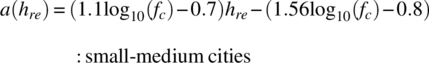
and for large cities

For suburban and open rural areas, the correction factors are

and

19.8.3 Erceg Model for Suburban and Rural Environments
The Erceg model [25] characterizes the loss for wireless mobile communication in suburban and rural areas. The results are based on curve‐fit plots of loss vs. distance derived from 1.9 GHz experimental data collected in 95 macro cells across the United States. In this case, the data was collected using omnidirectional azimuth antennas with transmit and receive gains of 8.14 dB and 2.5 dB respectively. The receiver antenna height was fixed at hr = 2 m.
This model is directed toward applications, like personal communication services (PCS) that involve smaller cells, lower transmit antenna heights and higher frequencies. The path loss applies for transmitter effective antenna heights: 10 m ≤ hte ≤ 80 m and distances in the range: 0.1 m ≤ d ≤ 8 km. The three environments include various terrain hill conditions and tree densities. The Erceg model loss is expressed as

where do = 100 m is the minimum close‐in distance. The exponent γ is a Gaussian random variable expressed as5
where, the term in brackets, and σγ are the mean and standard deviation of γ respectively. The parameter x is a normalized Gaussian random variable characterized as N(0,1).6 The s term in (19.65) is a zero‐mean Gaussian random shadow fading term characterized as N(0,σ) and expressed as
where y = N(0,1), z = N(0,1), and σ is a Gaussian random variable characterized by N(μσ,σσ). The variables x, y, and z are independent random variables. The constants a, b, c, σγ, μσ, and σσ are listed in Table 19.5 for each terrain category.
TABLE 19.5 Numerical Values for Model Parametersa
| Parameter | Terrain Categoryb | ||
| A | B | C | |
| a | 4.6 | 4.0 | 3.6 |
| b (m−1) | 0.0075 | 0.0065 | 0.005 |
| c (m) | 12.6 | 17.1 | 20.0 |
| σγ | 0.57 | 0.75 | 0.59 |
| μσ | 10.6 | 9.6 | 8.2 |
| σσ | 2.3 | 3.0 | 1.6 |
aErceg et al. [25]. Reproduced by permission of IEEE.
bA, hilly with moderate to heavy tree density; B, hilly with light tree density or flat with moderate to heavy tree density; C, flat with light tree density.
19.9 LAND MOBILE SATELLITE PROPAGATION LOSS MODELS
Land mobile communications through a satellite must consider the loss from the terrain surrounding the mobile location. For example, in suburban and rural areas, when traveling along roads or walking in forested regions, foliage attenuation from trees and vegetation may result in significant signal losses. Link margins of 20–25 dB are recommended at ultra‐high frequency (UHF) for satellite viewing at elevation angles on the order of 20° or less.
Several link loss models for the suburban and rural areas are examined in the following sections. The underlying models are based on the modified exponential decay (MED) model introduced by Weissberger [26] with variations based on the recommendations of the Consultative Committee on International Radio7 (CCIR) [27]. Barts and Stutzman [28] have also proposed modification to the MED model. The CCIR link margin model [29] for urban, suburban, and rural areas is also given in Section 19.9.4. Moraitis, Milas, and Constantinou [30] compare these and other land mobile satellite channel models.
In the following loss models the distance Dn is the propagation path length through the foliage, measured in meters, with the restriction Dn ≤ 400 m. Furthermore, the frequency f is the carrier frequency in megahertz in the range 200–95,000 MHz. The loss for each of the models is evaluated at 400, 1,200, and 16,000 MHz corresponding to the UHF, L, and Ku bands. The link margin evaluation in Section 19.9.4 is characterized in term of the elevation angle θ from the mobile site to the satellite. In this case, the frequency is denoted in gigahertz and the elevation angle in degrees. The models are based on in situ measured data with regression curve fitting applied to evaluate various parameter coefficients.
19.9.1 Modified Exponential Decay Model Link Loss
The MED model applies to suburban and rural environments consisting primarily of trees and vegetation. The total loss through the foliage is evaluated as
where an is the specific attenuation expressed as
The losses are shown in Figure 19.22 for the indicated frequencies.

FIGURE 19.22 MED model link loss.
19.9.2 CCIR Link Loss Model
The CCIR model is a modification of the MED model with the total loss given by
and the specific attenuation expressed as
The loss using the CCIR model is shown in Figure 19.23 and is somewhat higher than that predicted by the MED model.

FIGURE 19.23 CCIR model link loss.
19.9.3 Barts and Stutzman Link Loss Model
The Barts and Stutzman model is also a modification of the MED model for distances ≤14 m; otherwise, the loss predictions are identical to the MED model. The total loss through the foliage is evaluated as
and the specific attenuations for the different ranges are expressed as
and
The loss for the Barts and Stutzman model is shown in Figure 19.24.

FIGURE 19.24 Barts and Stutzman model link loss.
19.9.4 CCIR Link Margin Model
The CCIR link margin model [29] data were collected in urban, semi‐urban, suburban, and rural areas at 860 MHz and 1.55 GHz for elevation angles [31] ranging from 19° to 43°. In the following relationships, the angles are entered as degrees and the frequency as gigahertz. The link margin applies for a percentage availability of Pa = 90%, that is, the received signal power exceeds the detection threshold 90% of the time; however, other percentages of availability can be evaluated by subtracting the loss L = 0.1(90 − Pa) dB from the derived link margins.8 The range of Pa is 50–90%. Furthermore, a factor K is included that relates the percentage of the surrounding locations or area (area%) for which the received power is expected to exceed the detection threshold; the values of K for area% are tabulated in Table 19.6.
TABLE 19.6 Values of the Factor K Given area%
| area% | K |
| 50 | 0 |
| 90 | 1.3 |
| 95 | 1.65 |
| 99 | 2.35 |
The link margin, in dB, for the urban, suburban, and rural models are expressed as

and

Equations (19.75) and (19.76) are plotted in Figure 19.25 as a function of θ for various carrier frequencies in gigahertz with the indicated conditions of: link availability, percent of area, and L = 0 dB. With Pa = 90%, area% = 50%, and K = 0, the link is available 90% of the time and in 50% of the surrounding area the received power is expected to exceed the detection threshold. If the availability is decreased to 50% then L = −4 dB and the link margin can be decreased by 4 dB. On the other hand, if the detection threshold is to be exceeded in over 99% of the surrounding area then K = 2.35 and the link margin must be increased by the additive term involving K in (19.75) and (19.76). Note that the range of the elevation angle in Figure 19.25 exceeds the stated range of the model by about 5° on each end of the abscissa. The frequency translations method of Goldhirsh and Vogel [32] is recommended to evaluate the link margin requirements at other frequencies.

FIGURE 19.25 CCIR link margins for urban, suburban and rural areas (Pa = 90%, area% = 50).
19.10 IMPULSIVE NOISE CHANNEL
19.10.1 Introduction
Impulsive noise occurs from thunder storm activity around the world and is present in most regions as the energy from lightning flashes or strikes propagates through the natural wave guide between the earth surface and the ionosphere. The severity of the storm activity varies with geographic regions and seasons; however, the worldwide average rate of lightning strikes is on the order of hundreds‐per‐second. In regions near active storm centers the noise spikes are most pronounced, characterized as short high‐energy pulses that disrupt communications. As the impulsive energy propagates farther from the storm center the wide bandwidth pulses undergo attenuation and dispersion and combine with similarly filtered impulses from storm centers in other regions of the globe. The global effects of lightning strikes resulting from storm activity are most evident at the lower frequencies, typically in the low frequency (LF) region and below. These effects become less troublesome at frequencies in the high frequency (HF); however, the HF region has unique issues [33] to contend with including time‐varying multipath, ducting, and Faraday rotation.
The impulsivity measure Vd is introduced in Chapter 14 as the parameter that characterizes the severity of the impulsive noise and is defined as the ratio of the rms noise envelope to the average noise envelope. The Vd measure is expressed in decibels with the minimum value of 1.049 dB corresponding to minimum storm activity; larger values indicate increased storm activity. As the storm energy from around the globe is combined, the noise addition is subject to the central limit theorem and the impulsive noise approaches white Gaussian noise with the corresponding Vd = 1.049 dB. This condition is observed during periods of relatively calm worldwide storm activity and will change suddenly as a result of a distance storm. The impulsivity is also characterized by the amplitude probability distribution (APD), defined as the probability that the noise envelope exceeds the abscissa [34]. The worldwide characterization of impulsive noise due to storm activity is published by the International Telecommunication Union (ITU) through the CCIR Report 322 [35] and associated reports [36]. These reports characterize the APD based on impulsive noise measurements corresponding to the Vd measure. The impulsive noise from lightning strikes is characterized as a nonstationary random process and the APD data are based on the ensemble average of recorded time sequences.
19.10.2 Lognormal Impulse Noise Model
To the casual observer, a lightning strike appears as a single flash of light; however, in many events each flash is actually composed of multiple strokes separated typically by 50–100 ms. The multiple strokes following the initial lightning strike are referred to as return strokes. The number and interval between the return strokes is modeled statistically based on observations [37]. Uman and Krider [38] have summarized the phenomenon of lightning strikes and, based on the studies of Mackerras [39], conclude that the number of return strokes is typically distributed between 2 and 8 resulting in a mean value of 5 return strokes for each lightning flash. Figure 19.26 shows Mackerras’ results in terms of the probability that the number of return stokes exceeds the abscissa; the dashed curve represents the piece‐wise linear approximation to the data expressed in (19.77) and is used in the computer simulations. Beach and George [40] and Uman [41] report on the time between return strokes based on the data collected by Schonland in South Africa. Figure 19.27 characterizes Schonland’s data in terms of the probability that the time interval between return strokes exceeds the abscissa; the dashed curve corresponds to a piece‐wide linear approximation in (19.78) used for computer simulations. Beach and George observed that the time between stokes corresponding to Schonland’s data can be approximated using the Gamma pdf with α = 2 and mean value α/β = 55. This approximation is also applied to the data of Kitagawa, Brook, and Workman [42] for cloud‐to‐ground lightning using a mean value of α/β = 35. Although these Gamma function pdf approximations are good fits to the data over regions about the mean values, over regions several standard deviations removed from the mean they are not as accurate, so the piece‐wise linear approximations are used in the computer simulations.

FIGURE 19.26 Number of return strokes.
Mackerras [39]. Courtesy of the American Geophysical Union (AGU).

FIGURE 19.27 Time interval between return strokes.
The piece‐wise linear approximations for the simulated probabilities are

and

where j and n are integers and the time is in milliseconds.
The impulse noise for lightning strikes is modeled as shot noise [43] and expressed as the summation
where Np(t) represents the main lightning stroke with the associated return strokes, ![]() , and is expressed as
, and is expressed as
with
The functions Np(t) and ![]() represent complex impulse noise processes with lognormal distributed amplitudes Ap(t),
represent complex impulse noise processes with lognormal distributed amplitudes Ap(t), ![]() and uniformly distributed phases, φ(t), φ′(t), respectively.
and uniformly distributed phases, φ(t), φ′(t), respectively.
From the discussions in Section 14.3.6, the lognormal amplitude is Ap = ex, where x is a normally distributed random variable with mean m0, variance ![]() , and phase φ uniformly distributed between −π and π. A zero mean Gaussian background noise term, ng(t), with variance
, and phase φ uniformly distributed between −π and π. A zero mean Gaussian background noise term, ng(t), with variance ![]() is added to the impulsive noise; the background noise results from quiescent worldwide thunder storm activity. Therefore, the total atmospheric noise at the input to the receiver antenna is described as
is added to the impulsive noise; the background noise results from quiescent worldwide thunder storm activity. Therefore, the total atmospheric noise at the input to the receiver antenna is described as
Substituting (19.80) and (19.81) into (19.79) the total atmospheric noise at the receiver antenna input, characterized by (19.82), becomes9

The most commonly observed lightning strike or flashes occur as intra‐cloud, cloud‐to‐cloud, and cloud‐to‐ground.10 To the casual observers the cloud‐to‐ground lightning is the most spectacular. In cloud to ground flashes the first or main strike is preceded by a stepped leader that is followed by dart leader that propagates from the cloud to ground. The dart leader is immediately followed by a return stroke that propagates from ground to cloud and results in the visible lightning flash. Depending on the remaining charge and the electric field intensity, additional dart leaders followed by return strokes may occur resulting in a multiple‐stroke flash. In the communication performance simulation program, the parameter λ is input to establish the mean lightning flash‐rate. The time intervals Δti = ti − ti−1 between multiple return strokes are randomly distributed according to (19.78). As discussed in Section 19.10.3, the number of strokes and flashes over a recorded ensemble of atmospheric noise is adjusted to match the APD corresponding to the selected Vd (dB).
Two points are noteworthy regarding the noise description in (19.83). The implied bandwidth of the noise impulses is infinite and in areas of intense storm activity the parameter λ may be sufficiently high so that return strokes from several main strokes overlap. The bandwidth issue is handled by passing the impulse noise through the receiver intermediate frequency (IF) filter with one‐sided bandwidth denoted by B. The resulting received atmospheric noise at the output of the IF filter is then evaluated as
where h(t) is the impulse response of the IF filter where the asterisk (*) denotes convolution. Regarding the second point, parameter λ is selected to conform to measured data to result is the prescribed APD.
19.10.3 Fitting the Noise Model to Measured Data
In a simulation model the required sampling frequency fs is chosen to conform to the receiver Nyquist sampling criterion. For example, when simulating the performance of a communication system using analytic signal representations, the sampling frequency is selected such that fs ≥ 2B, where B is the bandwidth of the received signal. In this regard, the sampling frequency is selected to result in an acceptably low loss resulting from the detected symbol energy and aliasing distortion. The received samples are processed in the demodulator for waveform acquisition and subsequently symbol and carrier tracking and data detection. In this context t = kTs: Ts = 1/fs and (19.84) is the narrowband analytic representation of the received atmospheric noise. For evaluating the communication performance, the modulation symbol rate and the sampling frequency are related to the anti‐aliasing filter bandwidth B as shown in Figure 19.28.

FIGURE 19.28 Relationship between fs, B, and Rs for MSK modulation.
In the following evaluation of the impulse noise model, a minimum shift keying (MSK)‐modulated waveform is used with a symbol rate of Rs = 25 sps, B = 800 Hz, fs = 2B, and Ns = 32 samples‐per‐symbol. Because λ has units of impulses per second, the impulse rate is restricted to ![]() so the parameter Ns can be adjusted as necessary to fit the noise model to the measured data. These relationships are scaled to accommodate specific waveform modulations and data rates as discussed in the case study in Section 19.10.5.
so the parameter Ns can be adjusted as necessary to fit the noise model to the measured data. These relationships are scaled to accommodate specific waveform modulations and data rates as discussed in the case study in Section 19.10.5.
Lightning strikes are characterized by the impulsivity measure Vd defined in (14.67) as

where ![]() represents the narrowband time‐sampled receiver analytic noise. The system performance is typically characterized for a specified value of Vd; however, the APD for each Vd must conform to the corresponding measured APD in the ITU publication CCIR 322 [35]. To this end, the measured APD results are shown in Figure 19.29 for several values of Vd; these results are adapted from Gamble [44] and plotted using Rayleigh coordinates that result in a linear APD curve with slope −1/2 for Gaussian noise. The CCIR APD results are measured at the output of a receive antenna modeled as a single‐pole filter with a noise bandwidth of Bn = 243 Hz. Therefore, when specifying Vd in (19.85) the parameters
represents the narrowband time‐sampled receiver analytic noise. The system performance is typically characterized for a specified value of Vd; however, the APD for each Vd must conform to the corresponding measured APD in the ITU publication CCIR 322 [35]. To this end, the measured APD results are shown in Figure 19.29 for several values of Vd; these results are adapted from Gamble [44] and plotted using Rayleigh coordinates that result in a linear APD curve with slope −1/2 for Gaussian noise. The CCIR APD results are measured at the output of a receive antenna modeled as a single‐pole filter with a noise bandwidth of Bn = 243 Hz. Therefore, when specifying Vd in (19.85) the parameters ![]() ,
, ![]() , m0, and λ of the filtered noise process characterized by (19.83) and (19.84) must be chosen to conform to the corresponding APD curve. The parameter λ is implicit in (19.83) through the random distribution of the time between the lognormal impulses. The parameters m0 and
, m0, and λ of the filtered noise process characterized by (19.83) and (19.84) must be chosen to conform to the corresponding APD curve. The parameter λ is implicit in (19.83) through the random distribution of the time between the lognormal impulses. The parameters m0 and ![]() are implicit in the normally distributed random variable x denoted as x = N(m0,σ0).
are implicit in the normally distributed random variable x denoted as x = N(m0,σ0).

FIGURE 19.29 APD curves corresponding to CCIR‐322 measured Vd values (243 Hz receive filter noise bandwidth).
An analytic closed‐form solution for Vd in terms of the model parameters is intractable because of the denominator term in (19.85) involving the expectation of the magnitude of the received noise. Therefore, Vd is evaluated numerically in terms of ![]() ,
, ![]() , m0, and λ with the background noise power based on a specified receiver signal‐to‐noise ratio11 γb = Eb/No as
, m0, and λ with the background noise power based on a specified receiver signal‐to‐noise ratio11 γb = Eb/No as

where Vr is the peak voltage of the carrier‐modulated received signal. Upon specifying ![]() , λ, and m0, (19.85) is evaluated by indexing
, λ, and m0, (19.85) is evaluated by indexing ![]() : n = 1, …, N until the computed value of Vd just exceeds the specified value. Each evaluation involves a time series of one million samples to compute the expectations required in (19.85).12 The starting value of
: n = 1, …, N until the computed value of Vd just exceeds the specified value. Each evaluation involves a time series of one million samples to compute the expectations required in (19.85).12 The starting value of ![]() , denoted as
, denoted as ![]() , is chosen to minimize the search time and
, is chosen to minimize the search time and ![]() was found to provide sufficient coarse resolution to match the desired APD curve. However, to improve the estimation accuracy, a fine resolution interval of
was found to provide sufficient coarse resolution to match the desired APD curve. However, to improve the estimation accuracy, a fine resolution interval of ![]() is used with the indexing restarted at the previous value and continuing with
is used with the indexing restarted at the previous value and continuing with ![]() :
: ![]() until the computed value of Vd again exceeds the specified value. Upon completion, the value
until the computed value of Vd again exceeds the specified value. Upon completion, the value ![]() is linearly interpolated between the ending and previous values and the simulation is run once again to verify the evaluation of the desired APD curve using the four parameter values.
is linearly interpolated between the ending and previous values and the simulation is run once again to verify the evaluation of the desired APD curve using the four parameter values.
The final simulation run uses the interpolated value of ![]() and the numerically computed error in Vd in decibels is typically less than 0.1%. The final parameter sets for several Vd values are summarized in Table 19.7. The results of the Vd and APD evaluations are shown as the data points in Figure 19.30 for Vd values of 1.049, 2, 6, and 14 dB; the solid curves are taken from Figure 19.29 and represent the corresponding measured APD curves.
and the numerically computed error in Vd in decibels is typically less than 0.1%. The final parameter sets for several Vd values are summarized in Table 19.7. The results of the Vd and APD evaluations are shown as the data points in Figure 19.30 for Vd values of 1.049, 2, 6, and 14 dB; the solid curves are taken from Figure 19.29 and represent the corresponding measured APD curves.
TABLE 19.7 Lognormal Parameter Sets Corresponding to Selected Vd Values
| Vd (dB) | λ | m0 | γb | ||||
| 1.049 | — | — | Any | Any | — | — | — |
| 1.5 | 1150 | 0 | 36.5 | 1.120(−4) | 0.2074 | 0.0163 | 0.0035 |
| 2.0 | 300 | 0 | 28.0 | 7.920(−4) | 0.7625 | 0.1000 | 0.0212 |
| 6.0 | 3000 | 0 | 15.0 | 0.01581 | 2.218 | 2.0500 | 0.4400 |
| 14.0 | 1500 | 3 | −30.0 | 500.00 | 4.726 | 5.483(3) | 1.354(4) |
aApplies to MSK matched filter.

FIGURE 19.30 Simulated APD characteristics for several values of Vd using lognormal model (parameter sets from Table 19.7).
Figures 19.31, 19.32, and 19.33 show typical recordings of the sampled magnitude, ![]() , of the lognormal impulse noise for Vd = 1.049, 2.0, and 14.0 dB, respectively. These recordings are representative of the filtered samples at the output of the 243 Hz noise bandwidth receive antenna used to collect the CCIR‐322 noise data.
, of the lognormal impulse noise for Vd = 1.049, 2.0, and 14.0 dB, respectively. These recordings are representative of the filtered samples at the output of the 243 Hz noise bandwidth receive antenna used to collect the CCIR‐322 noise data.

FIGURE 19.31 Channel impulse noise record: Vd = 1.049 dB.
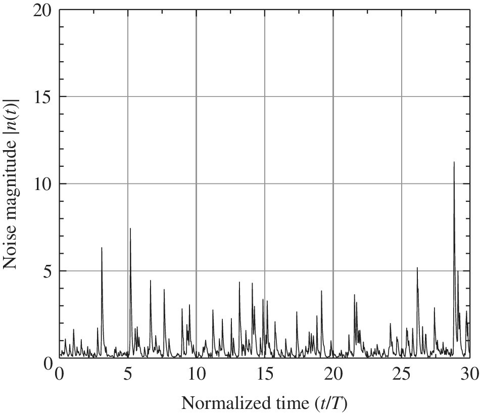
FIGURE 19.32 Channel impulse noise record: Vd = 6 dB.

FIGURE 19.33 Channel impulse noise record: Vd = 14 dB.
The value of Vd will change as the filter bandwidth is changed but the CCIR‐322 results apply only to the 243 Hz noise bandwidth filter [45]. Spaulding, Roubique, and Crichlow [46] have evaluated the conversion of Vd with bandwidth and their results are shown in Figures 19.34 and 19.35 for decreasing and increasing bandwidths respectively. Bi = Bn = 243 Hz is the noise bandwidth in which Vdi is measured and Bo is the noise bandwidth of the desired filter. The case study in Section 19.10.5 uses Bi = Bn = 243 Hz with Bo = Bn so no bandwidth conversion is necessary.13

FIGURE 19.34 Vd dependence on bandwidth: Bo/Bi ≤ 1. Spaulding et al. [46].
Courtesy Journal of Research of the National Bureau of Standards.

FIGURE 19.35 Vd dependence on bandwidth: Bo/Bi ≥ 1. Spaulding et al. [46].
Courtesy Journal of Research of the National Bureau of Standards.
19.10.4 Impulsive Noise Mitigation Techniques
Modem performance improvements can be achieved through the use of various impulsive noise mitigation techniques like: clipping [47], limiting [48], excision, and hole‐punching [49]. These techniques are applied in the receiver or demodulator signal path prior to the matched filter detection; however, at the outset of the modem design, the proper selection of the waveform modulation and forward error correction (FEC) coding will result in significant performance advantages. When FEC is applied to the waveform, the use of interleaving is also an effective mitigation technique for impulsive noise. Gamble [44] provides a review of these subjects and summaries the performance results of various authors for constant amplitude waveform modulations: PSK, MSK, and continuous phase frequency shift keying (CPFSK). In Section 19.10.5, the performance improvement using clipping is examined using the MSK‐modulated waveform. Time domain clipping is most effective when applied at a high IF frequency before significant pulse dispersion occurs; this can be achieved for constant envelope waveforms with bandpass limiting followed by narrowband filtering.
19.10.5 Case Study: Minimum Shift Keying Performance with Lognormal Impulse Noise
This case study involves simulating the performance of MSK operating as a bit‐rate of Rb = 50 bps in lognormal noise representative of lightning strikes from worldwide storm centers. In the preceding sections, the parameter Vd is used to characterize the receiver noise described by (19.84). The application of (19.84) involves generating noise samples ![]() , where Ts is the sampling interval, and combining the noise samples with the sampled signal (si) as shown in Figure 19.36. The sampling frequency fs = 1/Ts must be chosen to satisfy the Nyquist sampling condition.
, where Ts is the sampling interval, and combining the noise samples with the sampled signal (si) as shown in Figure 19.36. The sampling frequency fs = 1/Ts must be chosen to satisfy the Nyquist sampling condition.

FIGURE 19.36 Application of impulse noise for modem performance evaluation.
The receiver filter in Figure 19.36 represents the cascade of receiver and demodulator IF filters with a composite noise bandwidth of B Hz. The bandwidth of the single‐pole filter following the impulse noise generator establishes the impulsivity measure ![]() and the corresponding APD for the system evaluation. For example, suppose that the receiver being evaluated has an antenna noise bandwidth of 486 Hz, referring to Figure 19.35 with Bo/Bi = 2, a value of Vd = 6 dB in 243 Hz corresponds to
and the corresponding APD for the system evaluation. For example, suppose that the receiver being evaluated has an antenna noise bandwidth of 486 Hz, referring to Figure 19.35 with Bo/Bi = 2, a value of Vd = 6 dB in 243 Hz corresponds to ![]() = 8 dB in the receiver noise bandwidth. Therefore, the system performance is evaluated using
= 8 dB in the receiver noise bandwidth. Therefore, the system performance is evaluated using ![]() = 8 dB with the corresponding APD response. However, in this case study, Bi = Bn = 243 Hz with Bo = Bn, so the measured Vd values can be used without applying bandwidth conversion. This avoids the uncertainty introduced in the bandwidth conversion processing [46].
= 8 dB with the corresponding APD response. However, in this case study, Bi = Bn = 243 Hz with Bo = Bn, so the measured Vd values can be used without applying bandwidth conversion. This avoids the uncertainty introduced in the bandwidth conversion processing [46].
The signal must be passed through the equivalent receiver filters and the signal and intersymbol interference (ISI) distortion losses must be considered. Although the simulated signal is characterized as an analytic signal, the modulated signal at the filter output has an equivalent carrier‐modulated peak level of Vr volts corresponding to the signal power Ps = ![]() /2. Similarly, the power of the zero mean sampled noise is computed as
/2. Similarly, the power of the zero mean sampled noise is computed as

This power is measured in the bandwidth of the sampling frequency and the signal‐to‐noise ratio in the sampling bandwidth is Ns = fs/Rs times higher than Eb/No. In an environment involving white noise the channel power can be scaled by the bandwidth ratio and adjusted to correspond to a specified Eb/No ratio. However, because the impulse noise does not have a constant power spectral density (PSD) the signal will necessarily involve the channel noise power (![]() ) at the output of the symbol matched filter. For MSK modulation, the matched filter noise bandwidth is
) at the output of the symbol matched filter. For MSK modulation, the matched filter noise bandwidth is

The noise powers ![]() and
and ![]() are listed in Table 19.7 for the indicated values of Vd. The performance simulation evaluates the bit‐error probability as a function of the signal‐to‐noise ratio, γb = Eb/No measured in the bandwidth to the data rate Rb, that is,
are listed in Table 19.7 for the indicated values of Vd. The performance simulation evaluates the bit‐error probability as a function of the signal‐to‐noise ratio, γb = Eb/No measured in the bandwidth to the data rate Rb, that is,
Upon expressing (19.89) in terms of the noise power ![]() measured in the bandwidth Bmf and solving for
measured in the bandwidth Bmf and solving for ![]() results in
results in

Using (19.90) the voltage gain required to bring ![]() up to the level
up to the level ![]() for a specified γb = Eb/No is
for a specified γb = Eb/No is

This gain is applied to the simulated impulse noise as shown in Figure 19.36. As stated above, in the following simulations the input filter is the single‐pole filter with a noise bandwidth of Bi = 243 Hz used to characterize the CCIR‐322 data collection hardware.
Following the impulse noise gain adjustment, the received signal, receiver thermal noise, and impulsive channel noise are added and passed through the receive filter, the optional nonlinearity, and the MSK matched filter. The demodulator data estimates are determined from the optimally sampled matched filter and the errors are counted to determine the bit‐error probability. The hard limiting (HL) is ideal, in that, it normalizes the complex baseband signal plus noise (srk) as
When clipping is used, the clipping threshold is defined relative to the channel noise power ![]() and, because the received signal power is held constant, the clipping level (CL) relative to the received signal voltage Vr is also constant. The matched filter is a complex inphase and quadrature (I/Q) filter with quadrature cosine weighed symbol integrators offset by the bit duration Tb = T/2, where T is the MSK symbol duration. Ideal symbol timing is used, however, the performance using ideal frequency and phase tracking is compared to the performance using a second‐order Costas phaselock loop with various time‐bandwidth products.
and, because the received signal power is held constant, the clipping level (CL) relative to the received signal voltage Vr is also constant. The matched filter is a complex inphase and quadrature (I/Q) filter with quadrature cosine weighed symbol integrators offset by the bit duration Tb = T/2, where T is the MSK symbol duration. Ideal symbol timing is used, however, the performance using ideal frequency and phase tracking is compared to the performance using a second‐order Costas phaselock loop with various time‐bandwidth products.
The following figures characterize the performance of the MSK‐modulated waveform for various Vd values as described above. The modulation symbol rate of Rs = 25 sps has negligible distortion when passed through the single‐pole equivalent receiver antenna filter. The receiver bandwidth of B = 800 Hz is sufficiently wide to provide for effective clipping of the impulse noise peaks and the associated reduction of the Vd through clipping, HL, or bandwidth reduction is reflected in the performance results.
Gamble [44] has evaluated the theoretical performance of coherently detected binary phase shift keying (BPSK) with a linear receiver for various values of Vd. Gamble also provides comparisons of the theoretical performance with published experimental results for PSK [50] with Vd = 3.75 dB measured in 33.3 Hz and for MSK [51] with Vd = 5 dB measured in 40 Hz. These comparisons indicate the Gambles theoretical results provide a lower‐bound to the experimental results by 2–3 dB; however, the differences may be accounted for by measurement accuracies, tracking losses and other hardware anomalies. The simulation results in the following section focus on MSK modulation and compare reasonable well with Gambles results.
19.10.5.1 Simulated MSK Performance with Vd = 1.5 dB
The simulated performance of MSK in atmospheric noise with Vd = 1.5 dB and ideal symbol and phase tracking is shown in Figure 19.37. The performance using a linear receiver is compared to a HL receiver and a receiver with various CLs ranging from 0 to 21 dB. The Monte Carlo simulations use 1 M bits (500K symbols) for each signal‐to‐noise ratio and, because the channel noise does not have a constant power spectral density, the abscissa is defined more generally as ![]() .14 The dotted curve is the theoretical performance of MSK in additive white Gaussian noise (AWGN) and the circled data points (see Figure 19.38) result from the corresponding simulated performance. These ideal tracking performance results are provided as a baseline for comparison. The modem performance with impulsive noise is degraded from the AWGN performance by about 3.5 dB at Pbe = 10−5 with the linear receiver and an additional 0.2 dB with the HL receiver. The performance with CLs ranging from 0 to 21 dB fall between HL and linear performance.
.14 The dotted curve is the theoretical performance of MSK in additive white Gaussian noise (AWGN) and the circled data points (see Figure 19.38) result from the corresponding simulated performance. These ideal tracking performance results are provided as a baseline for comparison. The modem performance with impulsive noise is degraded from the AWGN performance by about 3.5 dB at Pbe = 10−5 with the linear receiver and an additional 0.2 dB with the HL receiver. The performance with CLs ranging from 0 to 21 dB fall between HL and linear performance.

FIGURE 19.37 Simulated performance of MSK in atmospheric noise (Vd = 1.5 dB, clipping, hard limiting and ideal tracking).

FIGURE 19.38 Simulated performance of MSK in atmospheric noise (Vd = 6 dB, clipping and ideal tracking).
The CL is defined in terms of the clipping threshold Tcl and the channel noise power ![]() as
as

The clipping threshold is related to the received signal power as

The signal power in the simulation is constant with Ps = 0.5 and, using the computed noise power from Table 19.7, ![]() = 0.0163, the clipping threshold relative to Ps in decibels is
= 0.0163, the clipping threshold relative to Ps in decibels is

Figure 19.37 also shows the performance with phaselock loop tracking using the time‐bandwidth product BLTb and lock detector BLDTb products of 0.025 and an initial phase error of 10° with zero frequency error. The critical phaselock loop signal‐to‐noise ratio of the linear receiver is about 8 dB and for the HL receiver it is about 14 dB. Clipping levels ranging from 0 to 21 dB were examined and the phaselock loop never achieved phase‐lock for CLs ≤ 18 dB. With CL = 21 dB phase‐lock was achieve with a critical signal‐to‐noise ratio of about 6 dB. Considering the CL relative to the signal power, as given by (19.95), the 21 dB CL corresponds to a clipping threshold relative to the signal power of 6.13 dB, whereas, CLs ≤ 18 dB correspond to clipping thresholds ≤3.13 dB relative to the signal power. These results indicate that an optimum clipping threshold exits with phase tracking. In all cases, once phase‐lock is achieved the performance loss is less than about 0.25 dB with tracking.
19.10.5.2 Simulated MSK Performance with Vd = 6 dB
The simulated MSK results for Vd = 6 dB are shown in Figures 19.38, 19.39, and 19.40. In these figures, the dotted curve is the theoretical performance of MSK in AWGN and the circled data point corresponded to the simulated MSK performance. The Monte Carlo simulations use 1 M bits (500K symbols) for each signal‐to‐noise ratio. The results in Figure 19.38 compare the performance of a linear receiver with one using HL and various CLs; all of these results use ideal symbol time and phase tracking. As predicted by Gamble the performance of the linear receiver is severely degraded; however, HL and CLs ≤ −6 dB provide significant improvements.

FIGURE 19.39 Simulated performance of MSK in atmospheric noise (Vd = 6 dB, hard limiting and PLL tracking).

FIGURE 19.40 Simulated performance of MSK in atmospheric noise (Vd = 6 dB, clipping and PLL tracking).
Referring to (19.94) and Table 19.7, ![]() = 2.05 and the clipping threshold relative to the signal power, Ps = 0.5, is expressed in decibels as
= 2.05 and the clipping threshold relative to the signal power, Ps = 0.5, is expressed in decibels as

Therefore, a CL of −6 dB corresponds to a clipping threshold of relative to the signal power level of 0.13 dB. The CLs of −3 and 0 dB, shown in Figure 19.38, also exhibit considerable improvement relative to the linear receiver. These CLs correspond to the respective clipping thresholds of 3.13 and 6.13 dB relative to the signal power.
The simulation results in Figure 19.39 show the performance of the linear receiver and the HL receiver with phase tracking indicated by the dash‐dot‐dot curves. The phaselock loop (PLL) BLTb and lock detector BLDTb products are 0.025 and the initial phase error is 10° with zero frequency error. The critical signal‐to‐noise ratio for phase‐lock is about 14 dB for the linear system and 6 dB for the HL receiver.
Figure 19.40 shows the phase tracking performance with clipping. With CL = 0 dB phase‐lock is achieved for signal‐to‐noise ratios less than 0 dB and with CL = −3 dB the critical signal‐to‐noise ratio is about 8 dB. For signal‐to‐noise ratios below about 6 dB the PLL never achieved phase‐lock. With CLs ≤ −6 dB phase‐lock was never achieved for any signal‐to‐noise ratio; this in contrasted with HL that did achieve phase‐lock as mentioned above. The loop bandwidth is directly related to the signal level into the PLL and, because the receiver gain following the limiting and clipping is not adjusted, the low signal level associated with low CLs may be attributed to the failure to achieve phase‐lock. In any event, the performance at lower signal‐to‐noise ratios is an important consideration with the use of FEC coding. In all cases, once phase‐lock is achieved the performance loss is less than about 0.25 dB with tracking. The phaselock performance can be improved by reducing the time‐bandwidth products at the expense of less tolerance to the dynamics of the encounter.
19.11 OCEAN WIND WAVE CHANNEL
19.11.1 Introduction
When communicating with submarines in deep ocean environments, the distortion introduced by surface waves driven by wind is a major factor that degrades the system performance. The impact of wind waves on the signal amplitude and phase is severe at very low frequency (VLF) and LF frequencies and in this section the signal distortion is analyzed and quantified in terms of the sea‐state conditions. The performance degradation is examined in a case study in Section 19.11.5 and signal processing techniques to mitigate the impact of the wave distortion are discussed.
In the real‐world environment, the received signal is corrupted by additive atmospheric noise as discussed in the preceding sections; however, the impulsivity of the atmospheric noise is decreased because of the narrowband filtering through the sea water. As the water depth increases, the Vd measure of the atmospheric noise approaches 1.049 dB corresponding to Gaussian noise. In addition to the filtered atmospheric noise, the noise at the receiver consists of additive thermal noise and man‐made interference noise from equipment that falls within the bandwidth of the receiver IF stages. In these cases, the performance loss is mitigated through the use of robust symbol modulations, FEC coding, interleaving, and adaptive interference cancellation techniques [52].
A theoretical characterization of wind waves is given by Kinsman [53] where, in Chapter 8, the Pierson‐Neumann theory is discussed leading to the Neumann wave‐height energy spectral density (EDS) characterization. An alternate expression of the wave‐height spectral density is based on the Pierson‐Moskowitz theory and the two spectrums are compared. These energy spectrums characterize the wave height for a fully developed sea after a period of sustained winds and that is not influenced by the ocean floor or surrounding shore lines. In other words, the sustained winds are over deep oceans with a large surface area or fetch. In addition to the introduction given by Kinsman, the U.S. Navy [54] provides a description of the growth and decay of waves. The wind wave characteristics are identified in terms of a sea‐state number [55, 56] as given in Table 19.8. In the following sections, the Neumann wave‐height energy EDS is used to compute random wave‐height temporal records; these records are seamlessly linked in a computer simulation program and used to distort the amplitude and phase of the communication waveform for the purpose of evaluating the communication link performance under various sea‐state conditions.
TABLE 19.8 Sea‐State Number and Wind Wave Parameters
| Sea‐State Number | ||||||||
| Parameter | 1 | 2 | 3 | 4 | 5 | 6 | 7 | 8 |
| Wind velocity (knots) | 5 | 12 | 16 | 18 | 24 | 28 | 34 | 42 |
| Average wave height (ft) | 0.18 | 1.4 | 2.9 | 3.8 | 7.9 | 11 | 19 | 31 |
| Average wave length (ft) | 6.7 | 40 | 71 | 90 | 160 | 212 | 322 | 492 |
| Average wave period (s) | 1.4 | 3.4 | 4.6 | 5.1 | 6.8 | 7.9 | 9.7 | 12 |
19.11.2 Neumann Wave‐Height Energy Spectrum
The EDS of wave height in a fully developed sea of unlimited depth, fetch, and time is characterized by Neumann [57] as

where g is the gravitational acceleration at sea level, found from experimental data to be 9.8106 m/s2, u is the wind velocity in meter per second, and ϖ is the angular frequency of the energy spectrum in radian per second. The constant 4.791 is determined from experimental data and has dimension of m2/s5. S(ϖ) has dimensions of square meter‐second and is plotted in Figure 19.41 in terms of the frequency f = ϖ/2π. The severity of the sea condition is designated by the sea‐state number and the corresponding wind velocity as indicated in Table 19.8. Figure 19.41 clearly demonstrates the impact of the wind velocity with an increase of five decades in the peak energy spectrum between sea‐states 1 and 8. The alternate wind wave spectral density is based on the Pierson‐Moskowitz wave theory [58] and expressed by (19.98) and shown in Figure 19.42.15 The Neumann characterization is less intense at the higher frequencies with a net shift in energy to the lower frequencies.


FIGURE 19.41 Neumann wave‐height energy spectrums.

FIGURE 19.42 Pierson‐Moskowitz wave‐height energy spectrums.
The integral of the wave‐height EDS is the wave energy and, for the Neumann spectral density, is evaluated as

Commonly used statistical measures of the wave height are [59]: the average height ![]() , the average of the 1/3 highest wave
, the average of the 1/3 highest wave ![]() , and the average of the 1/10 highest wave
, and the average of the 1/10 highest wave ![]() . Expressed in terms of the wave energy, these average wave‐height measures are given by
. Expressed in terms of the wave energy, these average wave‐height measures are given by
and
The constant 4.791 in (19.99) applies for wave heights between ![]() and
and ![]() . The wave energy and corresponding wave heights are listed in Table 19.9 for the sea‐state conditions.
. The wave energy and corresponding wave heights are listed in Table 19.9 for the sea‐state conditions.
TABLE 19.9 Wave Energy and Average Wave Heights for Neumann EDS
| Sea‐State | uk (knots)a | E (m2) | |||
| 1 | 5 | 0.0007 | 0.047 | 0.075 | 0.095 |
| 2 | 12 | 0.056 | 0.419 | 0.668 | 0.849 |
| 3 | 16 | 0.235 | 0.858 | 1.373 | 1.746 |
| 4 | 18 | 0.423 | 1.151 | 1.840 | 2.340 |
| 5 | 24 | 1.783 | 2.363 | 3.778 | 4.806 |
| 6 | 28 | 3.854 | 3.475 | 5.550 | 7.070 |
| 7 | 34 | 10.173 | 5.645 | 9.025 | 11.480 |
| 8 | 42 | 29.262 | 9.575 | 15.307 | 19.472 |
aIn (19.99) wind velocity u is meter per second so u = 0.5148 uk.
bMeters.
19.11.3 Wave‐Height Generation Using Neumann’s Energy Density Spectrum
In this section, the received signal phase and amplitude characteristics are examined at a point beneath the ocean’s surface under various sea‐state conditions using Neumann’s wave‐height EDS. The approach is similar to that described in Chapter 20 for the generation of Rayleigh fading signals and involves the uniform sampling of the wave‐height EDS and then using the inverse Fourier transform (IFT) to generate discrete‐time sampled wave data. The resulting record of finite wave data samples is extended to an arbitrary length by joining independently generated records in a seamless manner.16
The sampling conditions are depicted in Figure 19.43 using an Nfft − point radix‐2 fast Fourier transform (FFT). The wave EDS is bandlimited to B Hz and sampled at the sampling frequency fs = NfftΔf Hz with N samples over the EDS response, that is, B = NΔf. The temporal response of the sampled EDS is shown as the sampled wave record in Figure 19.43b. TB = 1/B is defined as the time‐constant of the wave temporal response and is related to the correlation time of the wave; there are N time‐constants for each record.

FIGURE 19.43 EDS sampling characteristics.
The parameter N is chosen such that there are about four samples within the 3‐dB bandwidth (B3) of the EDS so the frequency increment is Δf ≅ B3/4. The parameters B3 and B are determined from Figure 19.41 and the value of Δf is chosen to satisfy the condition

where B is chosen so that integrated alias distortion is more than 25 dB below the EDS in the bandwidth B. Using these results, the record duration Trec is computed as Trec = 1/Δf.
Referring to Figure 19.54a, the sampling frequency is selected to satisfy the Nyquist criteria fs = kB with k ≥ 2. Using this result and (19.103), the size of the FFT is determined as

where k = 2n: n ≥ 1. The minimum value of k results in the smallest FFT size of 2m+1 samples and selecting larger values of k increases the size of the FFT by decreasing size sample interval Δt, however, Δf and Trec remain unchanged. Therefore, for a given number of samples‐per‐symbol, increasing k results allows for more user symbols‐per‐record with fewer records required for the Monte Carlo performance simulations.17 These relationships are dependent on the modulated symbol duration T = 1/Rs that is typically less than TB. Table 19.10 identifies the selected parameters that are used for the various sea‐state conditions in the case study of Section 19.11.5 and Table 19.13 identifies the common symbol rate of 32 symbols‐per‐second used for each sea‐state condition.
TABLE 19.10 Wave Energy Density Spectrum Sampling
| Sea‐State | B3 (Hz) | B (Hz)a | Δf (Hz) | N | Trec (s) | Nfft |
| 1–3 | 0.150 | 2.0 | 1/32 | 64 | 32 | 4096 |
| 4–5 | 0.100 | 2.0 | 1/32 | 64 | 32 | 4096 |
| 6–8 | 0.043 | 0.5 | 1/64 | 32 | 64 | 8192 |
aChosen for aliased distortion greater than 25 dB below the integrated EDS over B Hz.
The complex samples of S(f) are generated using identically distributed zero‐mean independent complex Gaussian random variables b(nΔf): n = 0, …, N − 1 with variance ![]() . Although S(f) extents over all positive frequencies, the maximum frequency (N − 1)Δf is selected to result in negligible distortion due to aliasing. The sampling frequency increment Δf determines the record length given by Trec = 1/Δf. To simplify the notation, the complex samples b(nΔf) are defined in terms of bn as
. Although S(f) extents over all positive frequencies, the maximum frequency (N − 1)Δf is selected to result in negligible distortion due to aliasing. The sampling frequency increment Δf determines the record length given by Trec = 1/Δf. To simplify the notation, the complex samples b(nΔf) are defined in terms of bn as
and, letting i = {I,Q}, the pdf of the independent quadrature samples bni are characterized by N(0,σs). The discrete‐time samples of the wave‐height data h(t), t = mΔt, are obtained using the radix‐2 inverse fast Fourier transform (IFFT) with M = 1/(ΔtΔf) and are evaluated as

Because the wave function is real‐valued, the negative frequency response, that is, the response from fs/2 to fs = MΔf, is the complex conjugate of the positive frequency response; this property simplifies the evaluation of (19.106). Figure 19.44 shows a typical wave‐height record. The M‐sample record describing the wave heights hm is concatenated with other independently generated records to create arbitrarily long temporal wave‐height conditions for Monte Carlo performance simulations. The record concatenation uses a third‐degree polynomial in t, such that, the amplitudes and slopes are equal at the record boundary points. The boundary points are separated by the wave‐height correlation interval τc. The normalized correlation response is evaluated as

and the correlation time is defined as the time at which

FIGURE 19.44 Sea‐state 6 wave‐height record (N = 32, M = 8192).
With ![]() and
and ![]() the discrete‐time correlation function is evaluated as
the discrete‐time correlation function is evaluated as

Using (19.107) through (19.109) to determine the correlation time, the number of interpolation samples required to concatenate the wave‐height records is ![]() . Figure 19.45 shows a typical correlation response for sea‐state 6.
. Figure 19.45 shows a typical correlation response for sea‐state 6.

FIGURE 19.45 Sea‐state 6 wave correlation response (N = 32, M = 8192).
To demonstrate the fidelity of the wave‐height generation, the Fourier transform of the sea‐state 6 wave correlation response in Figure 19.45 is compared to the theoretical Neumann EDS. The results are shown in Figure 19.46 where the triangular data points represent the re‐constructed EDS for an average of 1000 ensembles or records. Figure 19.47 shows the reconstructed EDS with different sampling conditions for an average of 20 ensembles. Although a single ensemble will differ distinctly from the theoretical EDS, this is the nature of statistical sampling ensemble records as required for communications system performance evaluation.

FIGURE 19.46 Re‐constructed Neumann wave‐height energy spectrum (SS‐6, N = 250, M = 512, 1000 ensemble average).

FIGURE 19.47 Re‐constructed Neumann wave‐height energy spectrums (SS‐6, N = 32, M = 8192, 20 ensemble average).
19.11.4 Signal Generation using Temporal Wave‐Height Records
Having characterized the wave height for different sea‐state conditions, it is now necessary to solve for the sampled received signal with amplitude and phase temporal fluctuations [60] influenced by the changing height of the wind‐driven waves. The solution is found in the characterization of an electric field traversing the surface of a conducting medium expressed as [61]
where μ is the permeability and σ is the conductivity of the medium and ωc = 2πfc, where fc is the carrier frequency of the incident electric field Eo(t,ωc) in hertz. Typical values of μ and σ for sea water are: 4π10−7 H/m and 4 mho/m respectively; values of sea water conductivity range between 2 and 8 mho/m. Equation (19.110) is used to evaluate the fluctuations in the received signal with changes in the water depth due to the wave‐height variations h(t), described by (19.106). By noting that ![]() , the exponent in (19.110) is expressed as
, the exponent in (19.110) is expressed as
where18

The last equality in (19.112) is based on the above typical parameter values with fc expressed in hertz. Using (19.110) through (19.112), the temporal expression of a CW signal is
where A(t) and θ(t) are the wind wave‐dependent amplitude and phase functions given by
and
The attenuation A(t) results from the variation in the signal level due to the wave‐height temporal variations, however, (19.114) also expresses the static loss as the water depth (d) increases beneath the surface of the sea. This static attenuation or loss, expressed in decibel per meter, is given by

Equation (19.115) is plotted in Figure 19.48 as a function of the carrier frequency for various sea water conductivities.

FIGURE 19.48 Static signal attenuation through sea water.
The theoretical characteristics of the signal phase function are evaluated in terms of the derivatives of θ(t) using (19.115) with the result
The phase derivatives represent stochastic processes with correlation functions ![]() (τ) and corresponding phase energy EDSs are expressed as
(τ) and corresponding phase energy EDSs are expressed as

where
The phase variance is defined as

where E(n) is the energy of the derivatives of the wave height. Using (19.119) E(n) is evaluated as

Performing the integration in (19.121) using the Neumann EDS and substituting the result into (19.120) gives the standard deviation of the phase derivatives expressed as

The theoretical standard deviations expressed by (19.122) are listed in Table 19.11 for n = 0, 1, and 2 and Table 19.12 lists some corresponding results based on Monte Carlo simulation of the phase function as expressed by (19.115). The simulation results are based on eight wave‐height samples within the wave time‐constant TB depicted in Figure 19.43 with samples taken over 5 N time‐constants. Using a first‐order polynomial to link the records, the simulated results for ![]() resulted in discontinuities at the record boundaries. These discontinuities degrade the performance of PLL tracking with coherent demodulation; however, they can be eliminated by using a higher order polynomial for linking the records.19
resulted in discontinuities at the record boundaries. These discontinuities degrade the performance of PLL tracking with coherent demodulation; however, they can be eliminated by using a higher order polynomial for linking the records.19
TABLE 19.11 Theoretical Signal Phase Characteristics with Sea‐Statea
| Sea‐State Number | ||||||||
| Parameter | 1 | 2 | 3 | 4 | 5 | 6 | 7 | 8 |
| 1.04 | 9.31 | 19.11 | 25.65 | 52.66 | 77.42 | 125.8 | 213.4 | |
| 4.59 | 17.07 | 26.28 | 31.36 | 48.28 | 60.84 | 81.42 | 111.8 | |
| 35.00 | 54.22 | 62.61 | 66.40 | 76.68 | 82.83 | 91.27 | 101.4 | |
aNeumann spectrum corresponding to fc = 30 kHz.
TABLE 19.12 Simulated Signal Phase Characteristics with Sea‐Statea
| Parameter | Sea‐State Number | ||
| 2 | 4 | 6 | |
| 11.26 | 20.54 | 37.98 | |
| 16.87 | 14.10 | 31.85 | |
aNeumann spectrum corresponding to fc = 30 kHz.
The application of the wave amplitude and phase fluctuations, expressed in (19.114) and (19.115), respectively, to the received signal in a communication link is expressed in terms of the analytic signal representation as

where the transmitted analytic signal is expressed as
with
In these expressions, ![]() and
and ![]() are the modulation‐dependent amplitude and phase functions and Ps is the transmitted signal power.
are the modulation‐dependent amplitude and phase functions and Ps is the transmitted signal power.
The correlation response of a typical record of g(t) for sea‐state 6 is shown in Figure 19.49. Polar plots of the amplitude and phase fluctuations, in decibels and degrees, are shown in Figures 19.50, 19.51, and 19.52 for sea‐states 6, 4, and 2 respectively. Along the polar trajectory there are numerous phase reversals that are not apparent, for example, the occurrence of the first four phase reversals is indicated by the labeled arrows in Figure 19.50; the label 0 represents the record starting position. These phase reversals occur in the first quarter of the record and the entire record has 12‐phase reversals.

FIGURE 19.49 Sea‐state 6 signal correlation characteristics (N = 32, M = 8192, fc = 30 kHz).

FIGURE 19.50 Sea‐state 6 channel amplitude/phase characteristics for 64 second record (N = 32, M = 8192, fc = 30 kHz).

FIGURE 19.51 Sea‐state 4 channel amplitude/phase characteristics for 64 second record (N = 32, M = 4096, fc = 30 kHz).

FIGURE 19.52 Sea‐state 2 channel amplitude/phase characteristics for 64 second record (N = 32, M = 4096, fc = 30 kHz).
19.11.5 Case Study: Differentially Coherent BPSK Performance with Sea‐State
This case study examines the performance of differentially coherent BPSK (DCBPSK) waveform modulation with sea‐state distortion resulting from wind waves. The transmitted message is preceded by a single phase reference symbol that is used to detect the information bits. The ideal performance of DCBPSK in an AWGN channel is shown in Figure 19.53 and compared to the performance of coherent BPSK (CBPSK). The circled data points correspond to Monte Carlo simulated performance using 1 M bits for each signal‐to‐noise ratio. The following performance simulations with sea‐state examine the probability of receiving a 16‐bit word correctly so the word‐error probability is also plotted in Figure 19.53 under the ideal conditions involving AWGN. FEC coding is not used. These performance plots using the ideal AWGN channel are used for subsequent comparisons with the performance under various sea‐state conditions. The sea‐state simulations correspond to a carrier frequency of fc = 30 kHz.

FIGURE 19.53 Performance of DCBPSK in AWGN channel with comparison to coherent BPSK detection.
The criteria for the sampling of the temporal wave‐height records are outlined in Section 19.11.3 and the results are summarized in Table 19.10. Implicit in these requirements is the sampling of the communication waveform as determined by the selection of the FFT size. The most important consideration is that the selected sampling frequency results in an acceptable aliasing distortion loss. This condition requires that fs ≥ fN = 2(ρRs + |fe|) where fN is the Nyquist frequency, Rs is the transmitted symbol rate, fe is the maximum received carrier frequency error, and ρ is the number of spectral sidelobes permitted in the principal bandwidth |f| < fN/2. The aliased spectrum is depicted in Figure 19.54 as the dashed curves for the signal spectrum Ss(fT) = sinc(fT) with ρ = Ns = 4 and fe = 0.20 Although the FFT size is identified in Table 19.10 for the generation of the wave‐height samples, the selection criteria involve the symbol rate and the number of samples‐per‐symbol as characterized by
where the record length Trec = 1/Δf is determined in Section 19.11.3. Table 19.13 summarizes the selected FFT sizes for the various sea‐state conditions and the corresponding symbol rates with Ns = 4 samples‐per‐symbol. With these sampling conditions, the following bit‐error performance comparisons with sea‐state use identical symbol rates. Using 4 samples‐per‐symbol, as in this case study, the symbol rate can be increased by increasing the FFT size; however, this requires generating a new set of data records. On the other hand, the symbol rate can be decreased by simply increasing the samples‐per‐symbol without having to generate new sea‐state data records.21 The use of an integer number of samples‐per‐symbol is simply for convenience and avoids the necessity of rate conversion in the demodulator processing.

FIGURE 19.54 Modulated waveform sampling (shown for Ns = 4).
TABLE 19.13 Sampling Requirements and Modulation Symbol Rates
| Sea‐State | Trec (s) | Ns | Rs (sym/s) | Nfft |
| 1–3 | 32 | 4 | 32 | 4096 |
| 4–5 | 32 | 4 | 32 | 4096 |
| 6–8 | 64 | 4 | 32 | 8192 |
Figures 19.55 and 19.56 show the error performance for a DCBPSK‐modulated waveform with sea‐states 2, 4, and 6. Figure 19.55 corresponds to bit‐error probability using 1 M bits for each signal‐to‐noise ratio. The performance of antipodal and ideal DCBPSK operating in the AWGN channel are included for reference. When the waveform amplitude distortion, given by (19.114), is removed in the simulation, it is found that the performance is essentially unchanged indicating that the differentially coherent detection is predominantly impacted by the sea‐state phase distortion. The simulation conditions result in RsTB = 16, 32, and 64 symbols for each sea‐state time‐constant so increasing the symbol rate by about 8 : 1 or (32 : 1) should not result in a significant performance loss due to the phase distortion. The use of FEC coding and bit interleaving, with an interleaver span comparable to TB, will mitigate the performance loss resulting from wave fluctuations. Figure 19.56 shows the performance of DCBPSK‐coded message words with 8 and 16 bits‐per‐word.

FIGURE 19.55 Performance of DCBPSK with 16‐bit words with sea‐state conditions 2, 4, and 6 (fc = 30 kHz).

FIGURE 19.56 Performance of DCBPSK with 8‐ and 16‐bit words with sea‐state conditions 2, 4, and 6 (fc = 30 kHz).
19.12 LASER COMMUNICATIONS USING PHOTOMULTIPLIER DETECTOR
19.12.1 Introduction
A laser detector using a photomultiplier tube (PMT) [62] is shown in Figure 19.57. The collimated incident light waves (or photons) from the transmitter source are focused on the optical frequency filter and the desired filtered output illuminates the photosensitive surface of the photomultiplier tube releasing elections. The electrons are attracted to the photomultiplier anode by an electric field, created using the photomultiplier prime power, resulting in a current (is) through the load resistor RL. The current fluctuates with the source modulation as does the voltage across RL which is used to demodulate the source information. The gain of the photomultiplier is related to the number of free electrons at the anode relative to the energy of the incident light wave and gains on the order of 103 to 104 are not uncommon. The spatial filter eliminates light waves, entering the optical detector from directions other than from the communication transmitter [63, 64].

FIGURE 19.57 Photomultiplier optical detector.
The equivalent received signal power at the input to the PMT is denoted as Ps (Watts) and the current created by the PMT is determined as
where G is the gain of the PMT and S is the responsivity of the PMT defined as
where q is the electron charge = 1.602 × 10⁻¹⁹ C, η is the efficiency of the PMT, h is Planck’s constant = 6.62 × 10⁻³⁴ J‐s,22 and ν is the frequency in hertz.
The received signal power at the output of the PMT is the power delivered to the load resister and is computed as ![]() . Substituting (19.127) for is results in the received power
. Substituting (19.127) for is results in the received power
19.12.1.1 Photomultiplier Tube Noise Sources
The noise developed across the load resister results from several noise sources as described in this section.
DC or non‐fluctuating noise is defined in terms of the noise current ![]() ; therefore, the DC power into the load resistor is
; therefore, the DC power into the load resistor is
that behaves like the received signal power.
Thermal noise is determined by the system temperature Ts and is unaffected by the PMT gain; the two‐sided noise power density of the thermal noise is
Signal‐induced noise is shot‐noise resulting from the random release of electrons from the PMT optical surface. The shot‐noise is excited by the incident signal photons and results in the two‐sided noise power density expressed as
Background‐induced noise results from background light energy seen by the optical receiver. It consists of the Sun, Moon, bioluminescence, and other sources that are within the optical field of view (FOV); the two‐sided background noise power density is
Dark current noise results from shot‐noise caused by the random release of photoelectrons from the PMT optical surface due to the surface temperature. Although dark current noise encounters the gain of the PMT and it is usually negligible compared to the background induced noise and is often neglected. The dark noise power density is denoted as Nod.
19.12.1.2 Demodulator Signal‐to‐Noise Ratio
The following description is based on the M‐ary pulse position modulation (PPM) waveform format as shown in Figure 19.58. The symbol frame consists of a synchronization slot, containing the shaded transmitted laser pulse, followed by a dead‐time to provide for laser recharging, shown as the cross‐hatched interval, and M symbol slots that are selected based on the unique (log2M)‐bit data symbol. The transmitted laser pulses encounter dispersion through the channel and are depicted as the dotted received pulses. Selecting the slot duration of Ts seconds involves a tradeoff between several system design considerations. For example, in consideration of the pulse dispersion, increasing the slot duration increases the average received pulse energy capability at the detriment of the frame efficiency and message throughput. The dead‐time (Td) determines the pulse repetition frequency (prf) of the laser and is a major contributor to the frame overhead.23 The PPM parameters are examined in more detail in Section 19.12.3.

FIGURE 19.58 M‐ary PPM waveform symbol frame.
The demodulator post‐detection bandwidth is the reciprocal of the slot duration, that is, Bs = 1/Ts. The demodulator signal‐to‐noise ratio is defined in terms of the pulse energy, Ep = PLTs, as
The noise density is the sum of the noise sources discussed above, excluding the DC noise that is removed by the post‐detection filter, so the noise density is expressed as
Upon substituting (19.129) for PL, neglecting the dark and thermal noise sources, and substituting (19.135) with (19.132) and (19.133) into (19.134) results in

The responsivity (S) has units of amperes‐per‐watt, so the units of the product PS are amperes or coulombs‐per‐second. Therefore, since q is the electron charge with units of coulombs‐per‐electron, the quantity PS/q has units of electrons‐per‐second. In the following, the notation λ = PS/q is used and (19.136) simplifies to

where the second equality results by multiplying the numerator and denominator by Ts and recognizing that N = λTs is the number of photoelectrons in Ts seconds. Equation (19.137) is expressed in terms of the signal‐to‐noise ratio in the bandwidth equal to the bit‐rate, Rb = 1/Tb, using ![]() , where
, where
Upon solving (19.137) for Ns and expressing the result in terms of γb, the signal photoelectron count is evaluated as

These parameters are exactly those required to characterize the bit‐error performance of the demodulator in terms of the Poisson distribution as discussed in the following case studies [65, 66]. The photoelectron counting is also modeled using the Nakagami m‐distribution [67].
19.12.2 Pulse Dispersion in the Atmosphere
Based on experimental results [68–70], the generally accepted shape of a pulsed laser after emerging from clouds is shown in Figure 19.59 and characterized as

FIGURE 19.59 Received pulse shape through clouds.
In the following analysis, the PPM slot duration, measured in microsecond, is selected to satisfy two conflicting requirements: increase Ts to capture more received signal energy (Es) for detection or decrease Ts to provide the shortest PPM frame. The second of these options is dominated by the peak‐to‐average power ratio and the resulting duty cycle [71] of the laser transmitter. The laser pulse dispersion24 in the atmosphere results from the propagation path length (Lcp) through clouds and is characterized principally by the geometric thickness (Lcg) and the mean scattering angle (θcs) of the cloud. The delay (Tfd) and width (Tfw) of the integrate‐and‐dump (I&D) detection filter must be selected to maximize the signal‐to‐noise ratio at the optimum sample time of the detection filter. Communication links from the atmosphere to underwater links encounter additional dispersion that is dependent on the geometry of the encounter and the water type [72], for example [73], Jerlov II and III water25 and bioluminescence is a major source of background noise.
Stotts [74] has developed a closed‐form expression for laser pulse dispersion through clouds, for which, the pulse dispersion is expressed as

where c = 3e8 m/s is the free‐space speed of light, ωo > 0.999 is the cloud albedo26 (in the following analysis ωo = 1.0), τc is the optical thickness of the cloud,27 and Lcp and θcs are in meters and radians respectively. The relationship between the geometric cloud thickness (Lcg) and the optical cloud thicknesses is defined as
where σc is defined as the average extinction (or attenuation) coefficient of the cloud with dimensions of meters−1. The extinction coefficient is a measure of absorption of light in the cloud. In the following analysis σc = 0.04 m−1 which results in Lcg having dimensions of meters. The optical thickness of various types of clouds [75, 76] is listed in Table 19.14.
TABLE 19.14 Optical Thickness of Cloudsa
| Cloud Type | Optical Thickness | |
| Range | Average | |
| Cirrus, Altocumulus, Cumulus | 0–3.6 | 1.3 |
| Cirrostratus, Altostratus, Stratocumulus | 3.6–23 | 9.4 |
| Deep Convection, Nimbostratus, Stratus | 23–379 | 60 |
aInternational Satellite Cloud Climatology Project (ISCCP) 1983–2010 [76]. Courtesy of National Aeronautics and Space Administration (NASA).
Figure 19.60 is a plot of (19.141) showing the dependence of the pulse dispersion on the propagation path Lcp for the indicated mean scattering angles and average extinction of the cloud.

FIGURE 19.60 Laser pulse dispersion in clouds (σc = 0.04 m−1).
The pulse dispersion is measured as the pulse duration between the half‐power points of the pulse relative to the peak power Ppk that occurs at t = Tpk = 1/α. Defining the half‐power points of the pulse as occurring at T1 and T2, the pulse dispersion, expressed in (19.141), is Tcd = T2 − T1. Referring to Problem 23, T1 and T2 are related to the parameter α as T1 = 0.232/α and T2 = 2.677/α. Using these relationships, the pulse is completely characterized in terms of the dispersion through the cloud by the parameter α expressed as
Figure 19.61 shows the received pulse responses for the indicated values of the parameter Lcp, in kilometer, corresponding to the mean scattering angles used in Figure 19.60. In these plots, the received pulses are normalized by the total pulse energy Ep = 1/α2 resulting in unit energy pulses for each condition. Therefore, the integral

and E(Tcd)/Ep represents the normalized received pulse energy in the interval Tcd. Conversely, 1 − E(Tcd)/Ep represents the loss of energy in decibels.

FIGURE 19.61 Laser pulse shape in clouds.
Evaluating (19.144) over the range t = 0 to Ts, the received pulse energy in the PPM slot is determined as Es and is plotted in Figure 19.62 as a percent of the total received pulse energy. Figures 19.61 and 19.62 or Table 19.15 show that there is a large variation in Ts to cover the conditions; however, with θcs = 40° a slot duration of 23.3 µs will capture 95% of the pulse energy with Lcp = 1 km, whereas, a slot duration of 100 µs is required with θcs = 40 and Lcp = 2 km capture the same energy. If the transmitter can estimate the cloud conditions then Ts can be minimized and the receiver can form an estimate of the received slot duration during the waveform acquisition processing.

FIGURE 19.62 Percent of total pulse energy in slot duration.
TABLE 19.15 Slot Width to Capture Percent of Total Pulse Energy
| Es/Ep (%) | Loss (dB) | Ts (µs) | |||||
| Lcp = 1 km | Lcp = 2 km | ||||||
| 20a | 30 | 40 | 20 | 30 | 40 | ||
| 80 | 0.97 | 6.1 | 10.3 | 14.7 | 19.1 | 31.6 | 44.2 |
| 85 | 0.71 | 6.8 | 11.6 | 16.6 | 22.1 | 35.5 | 49.8 |
| 90 | 0.45 | 7.9 | 13.4 | 19.1 | 24.9 | 41.0 | 57.4 |
| 95 | 0.22 | 9.6 | 16.3 | 23.3 | 50.0 | 50.0 | 70.0 |
aThis row is θcs in degrees.
19.12.3 Pulse Position Modulation Waveform
The transmission of M‐ary coded data [77, 78] using a pulsed laser power source is often transmitted using PPM as described in Figure 19.58. The slot synchronization pulses are shown to occur prior to each M‐ary symbol location; however, for covert synchronization, they may occur at predetermined random locations known by the demodulator. Using periodic synchronization pulses simplifies the synchronize processing through the use of a narrowband bandpass filter centered at the synchronization pulse repetition rate; however, the use of FEC coding improves the bit‐error performance at the expense of increased complexity [79, 80]. Example FEC configurations are: a rate rc convolutional code with a prescribed constraint length, a Reed–Solomon code, for example a concatenated code with a constraint length K convolutional inner code and an M‐ary Reed–Solomon outer code with M = 2k bits per Reed–Solomon symbol. Data interleavers should also be used with FEC coding; especially between concatenated codes.
The source bit‐rate (Rb) of M‐ary PPM, without FEC coding, is expressed in terms of the bits‐per‐pulse (k) as

where k = log2(M). Equation (19.145) is plotted in Figure 19.63a and b as a function of k for Td = 5 and 1 ms respectively with the slot duration (Ts) as the parametric parameter. The laser dead‐time and the slot duration are seen to have a significant impact on the maximum data rate that also dictates the selection of k. The PPM waveform design, including the selection of the slot duration, bits‐per‐slot, and maximum user bit‐rate, are established using Figure 19.63. For example, using the 5 ms dead‐time shown in Figure 19.63a, and selecting k = 7 and Ts = 10 µs results in a 128‐ary PPM waveform with a maximum uncoded user bit‐rate of 1.113 kbps.

FIGURE 19.63 PPM bit‐rate.
Defining the slot duration as in Figure 19.59, the total received pulse energy in the slot and the percentage of pulse energy is determined from Figure 19.62 or Table 19.15. The optimum I&D detection filter delay and duration, shown in Figure 19.59, must be determined in the context of the statistical characterization of the PMT noise and other noise sources as discussed in Sections 19.12.1.1 and 19.12.1.2.
19.12.4 Differential Pulse Interval Modulation Waveform
With differential pulse interval modulation (DPIM) [81], the pulse intervals are synchronized to the transmission of an initial synchronization pulse followed by M‐ary coded pulses based on the differential change in the time slots relative to the preceding pulse. DPIM modulation is depicted in Figure 19.64 using the M‐ary coded waveform with symbol sequence (m, 5, 2, …). In this example, the DPIM‐coded waveform transmits the first information pulse in slot m following the reference pulse and the associated dead‐time, the second pulse is transmitted in slot five following the laser recovery of the first pulse, and the third pulse is transmitted in slot two following the laser recovery time. Therefore, the three information pulses are transmitted in a time equal to (m + 8)Ts + 3Td µs; whereas, the PPM‐modulated waveform, shown in Figure 19.58, transmits the first three information pulses in (3M + 1)Ts + 4Td µs. The average time to transmit a frame of M‐ary coded random data using the DPIM‐modulated waveform is

compared to ![]() µs for the PPM‐modulated waveform.
µs for the PPM‐modulated waveform.

FIGURE 19.64 M‐ary DPIM waveform symbol modulation.
Figure 19.65 shows the bit‐rate of DPIM as a function of the bits‐per‐slot under similar conditions for the PPM modulation shown in Figure 19.63. The average bit‐rate for DPIM is expressed as

FIGURE 19.65 DPIM average bit‐rate.
19.12.5 Case Study: PMT Demodulator Performance Using OOK Modulation
In this case study, the laser transmitter is either on‐off keying (OOK) resulting in the binary hypothesis in which a binary zero (b0) is represented by no signal energy being transmitted and a binary one (b1) is represented by transmitting a signal energy of Es. Under the maximum‐likelihood (ML) decision rule, the a priori probabilities are represented by P(b0) = P(b1) = 1/2 and the decision rule is expressed in terms of the transition probabilities using the likelihood ratio as

The transition probabilities are characterized in terms of the Poisson distributions [82]
where λi is the photoelectron rate and Ts is the interval in which the photoelectrons are counted, so Ni is the number of photoelectrons in Ts seconds. Under the conditions b1 and b0, the respective notations for the photoelectron counts are ![]() and
and ![]() . Ts is the reciprocal of the receiver post‐detection bandwidth and typically Ts ≅ Tb to allow for dispersion of the bit energy through the optical channel. Substituting (19.149) into (19.148) and rearranging the terms of the log‐likelihood ratio (LLR), the log‐likelihood ratio test (LLRT) is expressed, in terms of the threshold kT, as
. Ts is the reciprocal of the receiver post‐detection bandwidth and typically Ts ≅ Tb to allow for dispersion of the bit energy through the optical channel. Substituting (19.149) into (19.148) and rearranging the terms of the log‐likelihood ratio (LLR), the log‐likelihood ratio test (LLRT) is expressed, in terms of the threshold kT, as

This threshold is the optimum threshold for making the decision that minimizes the bit‐error probability, evaluated as

Pbe is evaluated in terms of γb by specifying the background photoelectron count Nb, and using (19.139) to determine Ns. The resulting bit‐error performance is shown in Figure 19.66 under ideal channel conditions with Ts = Tb and the indicated values of background noise. The bit‐error performance for Nb = 0 results in kT = 0 so Pbe simplifies to ![]() . The slight ripple in the Nb = 1 curve results from the integer summations involving the Poisson distributions; for threshold levels exceeding 14 the Gaussian approximation to the Poisson distributions is use to evaluate Pbe. The noncoherent OOK performance with AWGN is discussed in Chapter 6.
. The slight ripple in the Nb = 1 curve results from the integer summations involving the Poisson distributions; for threshold levels exceeding 14 the Gaussian approximation to the Poisson distributions is use to evaluate Pbe. The noncoherent OOK performance with AWGN is discussed in Chapter 6.

FIGURE 19.66 Bit‐error performance of OOK optical detector (Ts = Tb).
19.12.6 Case Study: PMT Demodulator Performance of M‐ary PPM Waveform
In this case study, the bit‐error performance is examined for the M‐ary PPM waveform [77] as characterized in Figure 19.58 with k = log2M bits transmitted in one of M time slots during each symbol frame of duration Tf = MTs + Td seconds. The laser pulse contained in the interval Tsync is used for frame synchronization and tracking. In this case, the ML decision rule uses equal a priori probabilities for each symbol with Pm = 1/M: ∀ m ∈ M. The rule that minimizes the symbol‐error probability selects the time slots having the largest post‐detection filter output when the post‐detection filter is matched to the received pulse. An upper bound on the symbol error is given by Bucher [83] as
where the exponent term Ec(Ns/Nb) is equal to

Solving (19.137) for Ns/Nb and substituting the result into (19.153) results in

As in the preceding binary example, the following performance is characterized in terms of the background noise count Nb; however, in this case, the independent variable will be the signal‐to‐noise ratio as measured in the slot bandwidth. Referring to (19.139), the parameter Ns is expressed in terms of Nb with the signal‐to‐noise ratio (γsym) measured in the symbol bandwidth equal to 1/T. Therefore, the signal photoelectron count, measured in the slot bandwidth, is computed as

where ![]() converts the signal‐to‐noise ratio from the symbol bandwidth to the signal‐to‐noise ratio in slot bandwidth.
converts the signal‐to‐noise ratio from the symbol bandwidth to the signal‐to‐noise ratio in slot bandwidth.
The M‐ary PPM performance is shown in Figure 19.67 as a function of γs for various values the background noise count Nb. The symbol‐error results are based on the union‐bound [84] which is a loose upper bound on the performance; however, for a fixed M, the union‐bound becomes increasingly tighter as γs increases. Figure 19.68 shows the union‐bound symbol‐error performance for the indicated values of k = log2(M) using a background photoelectron count of Nb = 200.

FIGURE 19.67 Symbol‐error performance of 256‐ary PPM optical detector (Ts = T).

FIGURE 19.68 Symbol‐error performance of M‐ary PPM optical detector (Nb = 200).
ACRONYMS
- AGU
- American Geophysical Union
- APD
- Amplitude probability distribution
- AWGN
- Additive white Gaussian noise
- BPSK
- Binary phase shift keying
- CBPSK
- Coherent BPSK
- CCIR
- Consultative Committee on International Radio
- CL
- Clipping level
- CPFSK
- Continuous phase frequency shift keying
- CW
- Continuous wave
- DCBPSK
- Differentially coherent BPSK
- DFT
- Discrete Fourier transform
- DPIM
- Differential pulse interval modulation
- EDS
- Energy density spectrum
- FEC
- Forward error correction (coding)
- FFT
- Fast Fourier transform
- FOV
- Field of view
- HF
- High frequency
- HL
- Hard limiting
- I/Q
- Inphase and quadrature (channels or rails)
- IF
- Intermediate frequency
- IFFT
- Inverse fast Fourier transform
- IFT
- Inverse Fourier transform
- ISCCP
- International Satellite Cloud Climatology Project
- ISI
- Intersymbol interference
- ITU
- International Telecommunication Union
- ITU‐R
- International Telecommunication Union‐Radio
- LF
- Low frequency
- LLR
- Log‐likelihood ratio
- LLRT
- Log‐likelihood ratio test
- LOS
- Line of sight
- MED
- Modified exponential delay (loss model)
- ML
- Maximum‐likelihood (decision rule)
- MSK
- Minimum shift keying
- NASA
- National Aeronautics and Space Administration
- PCS
- Personal communication services
- PMT
- Photomultiplier tube
- PLL
- Phaselock loop
- PPM
- Pulse position modulation
- TOD
- Time‐of‐day
- UHF
- Ultra‐high frequency
- VLF
- Very low frequency
PROBLEMS
- Establish the geometry for a ground‐to‐ground communication link using a flat Earth model with transmit and receive antenna heights ht and hr respectively. (a) Evaluate and plot the resulting received signal power density in terms of microwatts per square meter as a function of range for: ht = hr = 3 m, transmitter power Pt = 10 W, Gt = 3 dB and fc = 1 GHz. (b) Compare the results using the spherical Earth model in Figure 19.2 using the effective Earth radius re = (4/3)Re; assume that the Earth reflected multipath ray is negligible.
- Referring to Figures 19.1 and 19.2, given a transmitter height of h1, determine the minimum elevation angle θd(min) for a radio line‐of‐light path.
- Derive the expression for the average multipath loss
 defined in Section 19.4 in terms of the parameter
  . Express the result as a function of x.
 - Using the geometry shown in Figures 19.2 and 19.7 for a circular LEO satellite orbit with altitude h2 = 200 km and a ground antenna height of h1 = 30 m, derive an expression for the antenna elevation angle θd as a function of the satellite orbit angle θs.
- In Figure 19.2 consider the satellite to be at the height h2. At what angle, θd(min), will the satellite be in view of a ground antenna with h1 = 0?
- Using (16.3), with ε = 0 for a circular orbit, compute the satellite orbit time rate in second per degree. What is the viewing time of the satellite by the ground antenna over the interval θs(min) ≤ θs ≤ 90°?
- Plot the satellite viewing time as a function of the satellite orbit angle θs.
- By applying Huygens’ principle to Figure 19.4 use geometry to prove that the angle of reflection ϕr is equal to the angle of incidence ϕi.
- Evaluate the expressions (19.46), (19.48), and (19.52) for 0 and 100% relative humidity using an apparent elevation angle of αo = 15°, ψ = 120° with hg = 0 and ht = 50 K ft. Using hg and ht compute the corresponding refractive indices ng and nt using (19.42) through (19.45) and then compute the refraction angle error Δαo corresponding to the apparent elevation angle αo using Figures 19.14 and 19.15. Using these newly computed parameters determine the refractive angle error Δαt using (19.49); Δαt must be in radians. The final steps involve computing the Doppler frequency and frequency Doppler frequency error using (19.46) and (19.48). The Doppler frequency error is also to be expressed in the normalized form of (19.52) using the normalizing parameters fco = 100 MHz, Vo = 6.096 km/s. Note that these Doppler frequency expressions are what the aircraft terminal would encounter when attempting to receive a communication message; however, in a radar application the ground terminal radar would, because of reciprocity, experience twice these values over the two‐way path. Additional parameters necessary to complete this problem are: Re = 6378 km and c = 3 × 10⁸ m/s.
- Using the differential path length Δk = kλ/2 and the approximation given in (19.56): (a) derive the expression for the Fresnel zone radius hk and (b) show that the maximum Fresnel zone radius occurs when d1 = d2.
- For a knife‐edge obstruction with h1 = h2 = 30 m and a carrier frequency of 500 MHz, determine: (a) the diffraction loss for h = 12.76, 4.26, 0, −2.13, and −4.26 m, (b) in each case determine the Fresnel zone, k, of the obstruction, (c) comment on the significance of the Fresnel zones for h = 4.26 and −4.26 being identical given that the losses diffraction losses are significantly different.
- Using an effective transmit and receive antenna height of 1 and 10 m and a carrier frequency fc = 100 MHz, plot the normalized propagation loss in percent (100 Lp/Lfs) as a function of the range r = (0.5, 1, 2, 3, 4, 5) where Lp is the propagation loss computed using the Longley‐Rice Model and Lfs is the corresponding free space loss. For each range r use the following values of Lp corresponding to 100 MHz from Figure 19.19:
- Lp(he = 1 m) = (30.4, 37.7, 41.7, 45.7, 49.0, 51.7)
- Lp(he = 10 m) = (16.1, 21.2, 26.5, 29.8, 32.4, 34,5)
- Choose realistic heights for the transmit and receive antennas for a wireless mobile link and, using a base‐station or transmitter power of Pt = 10 W, and antenna gain Gt = 3 dB, compute, plot, and compare the received power density in microwatts per square meter as a function of distance d for the Okumura and Hata models described in Sections 19.8.1 and 19.8.2 using the suburban environments; for the Hata model use (19.63) for the suburban environment. Repeat the comparison using the open area environment; for the Hata model use the open rural environment loss expressed by (19.64).
- Choose a realistic transmit antenna height (ht) for a PCS link and use the ETAL model with a transmitter power of Pt = 10 W, antenna gain of Gt = 8.14 dB to evaluate and plot as a function of range the received signal power density in terms of microwatts per square meter for all three terrain categories listed in Table 19.5. Note: This model applies for a carrier frequency of fc = 1.9 GHz and a receiver antenna height of hr = 2 m.
- Show that the Rayleigh distribution p(r) results in a straight line with slope of −1/2 when plotted as log(ro/2σo) as a function of −log(−ln(P(r > ro))).
- Compute Vd for Gaussian noise.
- Using the equation for Gn, determine the clipping threshold voltage, Vth, relative to the received signal voltage Vr given that the clipping threshold relative to the channel noise standard deviation, σch, is k = Vth/σch, that is, determine k′ = Vth/Vr.
- Determine the noise bandwidth of the MSK matched filter.
- Evaluate the wave energy of the Pierson‐Moskowitz energy density function for sea‐states 1 through 8 and compare with that of the Neumann energy density function in Table 19.9.
- Beginning with equation (19.106) in the text, derive Equation (19.109).
- Show that
 has dimensions of meters−1.
 - Starting with the function θ(n)(t), defined in (19.117), express the autocorrelation
 in terms of the autocorrelation function
  .
. - Using the results of Problem 19, derive expression 19.119 in the text for the EDS S(n)(ω).
- Evaluate E(n) by performing the integration in (19.121) and using the result, verify the expression for the standard deviation
 given by (19.122) in the text.
 - Derive the coefficients for a second‐degree record linking polynomial y(xi) spanning m samples, such that i = 0, …, m with boundary conditions:
 ,
,  where yo and
  are the magnitude and slope of the last samples of the previous record and
  ,
,  where ym and
  are the magnitude and slope of the first samples of the next record.
 - Part a: Determine the time (Tpk) and the corresponding peak value pr(Tpk) of the received laser pulse expressed by (19.140). Part b: Determine the times T1 and T2, in terms of the parameter α, corresponding to the half‐power points pr(T1) and pr(T2) respectively.
Hint: Evaluate the resulting transcendental equation f(x): x = αt, for the two solutions using Newton’s method using initial guesses to the solution of x1(guess) < 1 and x2(guess) > 1. - Show that the Poisson distribution approaches the Gaussian distribution as M → ∞.
REFERENCES
- 1 D.E. Kerr, Editor, Propagation of Short Radio Waves, M.I.T. Radiation Laboratory Series, Vol. 13, McGraw Hill Book Company, New York, 1951.
- 2 L.E. Blake, Radar Range‐Performance Analysis, Munro Publishing Co., Silver Springs, MD, 1991.
- 3 P.L. Rice, A.G. Longley, K.A. Norton, A.P. Barsis, “Transmission Loss Predictions for Tropospheric Communication Circuits,” National Bureau of Standards Technical Note No. 101 Vol. 2, U.S. Department of Commerce, National Bureau of Standards, Washington, DC, May 7, 1965. Currently: National Institute of Standards and Technology (NIST).
- 4 L.E. Blake, Radar Range‐Performance Analysis, pp. 271–274, Munro Publishing Co., Silver Springs, MD, 1991.
- 5 C.R. Burroughs, S.S. Atwood, Radio Wave Propagation, Academic Press, New York, 1949.
- 6 D.K. Barton, Modern Radar System Analysis, pp. 297–280 and Appendix A, Artech House, Norwood, MA, 1988.
- 7 J.D. Kraus, Antennas, McGraw‐Hill Book Company, Inc., New York, 1950.
- 8 S. Ramo, J.R. Whinnery, Fields and Waves in Modern Radio, Chapter 7, John Wiley & Sons, Inc., New York, 1959.
- 9 L.E. Blake, Radar Range‐Performance Analysis, p. 259, Munro Publishing Co., Silver Springs, MD, 1991.
- 10 G.A. Hufford, A.G. Longley, W.A. Kissick, “A Guide to the Use of the ITS Irregular Terrain Model in the Area Prediction Mode,” U.S. Department of Commerce, Malcolm Baldrige, Secretary, April 1982.
- 11 E. Shotland, R.A. Rollin, “Complex Reflection Coefficient Over a Smooth Sea in the Micro and Millimeter Wave Bands for Linear and Circular Polarizations,” Report FS‐76‐060, John Hopkins University Applied Physics Laboratory, Laurel, MD, May 1976.
- 12 E.K. Smith, Jr., S. Weintraub, “The Constants in the Equation for Atmospheric Refractive Index at Radio Frequencies,” Proceedings of the Institute Radio Engineers (IRE), Vol. 41, No. 8, pp. 1035–1037, August 1953.
- 13 C.F. Campen, A.E. Cole, “Tropospheric Variations of the Refractive Index at Microwave Frequencies,” Air Force Surveys in Geophysics, No. 79, Geophysical Research Directorate, October 1955.
- 14 R.S. Berkowitz, Editor, Modern Radar, Analysis, Evaluation and System Design, Part V, Radio Frequency Considerations, Chapter 1, G.H. Millman, “Atmospheric Effects on Radio Wave Propagation,” John Wiley & Sons, Inc., New York, 1966.
- 15 R.S. Berkowitz, Editor, Modern Radar, Analysis, Evaluation and System Design, Part V, Radio Frequency Considerations, Chapter 1, G.H. Millman, “Atmospheric Effects on Radio Wave Propagation,” p. 341, Figure 1‐12, p. 342, Figure 1‐13, p. 344, Figure 1‐16, John Wiley & Sons, Inc., New York, 1966.
- 16 R.S. Berkowitz, Editor, Modern Radar, Analysis, Evaluation and System Design, Part V, Radio Frequency Considerations, Chapter 1, G.H. Millman, “Atmospheric Effects on Radio Wave Propagation,” p. 331, Figure 1‐4, p. 332, Figure 1‐5, John Wiley & Sons, Inc., New York, 1966.
- 17 M.I. Skolnik, Introduction to Radar Systems, McGraw‐Hill Book Company, Inc., New York, 1962.
- 18 D.K. Barton, Modern Radar Systems Analysis, Artech House, Inc., Norwood, MA, 1988.
- 19 W.C.Y. Lee, Mobile Communications Engineering, McGraw‐Hill Publications, New York, 1985.
- 20 M. Abramowitz, I.A. Stegun, Handbook of Mathematical Function with Formulas, Graphs, and Mathematical Tables, National Bureau of Standards, Applied Mathematics Series No. 55, U.S. Government Printing Office, Washington, DC, June 1964.
- 21 A.G. Longley, P.L. Rice, “Prediction of Tropospheric Radio Transmission Loss Over Irregular Terrain—A Computer Method,” Institute for Telecommunications Sciences, Environmental Science Services Administration, Boulder, CO, Technical Report ERL 79‐ITS 67, July 1968.
- 22 T.S. Rappaport, Wireless Communications: Principles and Practice, Prentice Hall PTR, Upper Saddle River, NJ, 2002.
- 23 T. Okumura, E. Ohmori, T. Kawano, K. Fukuda, “Field Strength and Its Variability in VHF and UHF Land Mobile Service,” Review Electrical Communication Laboratory, Vol. 16, No. 9–10, pp. 85–873, September–October 1968. Also appears in: Land‐Mobile Communications Engineering, Edited by D. Bodson, G.F. McClure, S.R. McConoughey, IEEE Press, Selected Reprint Series, pp. 19–67, 1984.
- 24 M. Hata, “Empirical Formula for Propagation Loss in Land Mobile Radio Services,” IEEE Transactions on Vehicular Technology, Vol. 29, No. 3, pp. 317–325, August 1980.
- 25 V. Erceg, L.J. Greenstein, S.Y. Tjandra, S.R. Parkoff, A. Gupta, B. Kulic, A.A. Julius, R. Bianchi, “An Empirically Based Path Loss Model for Wireless Channels in Suburban Environments,” IEEE Journal on Selected Areas in Communications, Vol. 17, No. 7, pp. 1205–1211, July 1999.
- 26 M.A. Weissberger, “An Initial Critical Summary of Models for Predicting the Attenuation of Radio Waves by Foliage,” ECAC‐TR‐81‐101, Electromagnetic Compatibility Centre, Annapolis, MD, August 1981.
- 27 Consultative Committee on International Radio (CCIR), “Influence of Terrain Irregularities and Vegetation on Tropospheric Propagation,” Report 236‐6, Vol. XIII‐3, Geneva, Switzerland, 1986. Currently: International Telecommunication Union‐Radio (ITU‐R).
- 28 R.M. Barts, W.L. Stutzman, “Modeling and Simulation of Mobile Satellite Propagation,” IEEE Transactions on Antennas and Propagation, Vol. 40, No. 4, pp. 375–382, April 1992.
- 29 Consultative Committee on International Radio (CCIR), “Factors Affecting the Choice of Antennas for Mobile Stations of the Land Mobile Satellite Service,” Report 925‐1, Vol. V, Geneva, Switzerland, 1986. Currently: International Telecommunication Union‐Radio (ITU‐R).
- 30 N. Moraitis, V. Milas, P. Constantinou, “On the Empirical Model Comparison for the Land Mobile Satellite Channel,” Institute of Communications and Computer Systems, National Technical University of Athens, Athens, Greece, 2007.
- 31 G.C. Hess, “Land‐Mobile Satellite Excess Path Loss Measurements,” IEEE Transactions on Vehicular Technology, Vol. 29, No. 2, pp. 290–297, May 1980.
- 32 J. Goldhirsh, W.J. Vogel, “An Overview of Results Derived from Mobile Satellite Propagation Experiments,” International Mobile Satellite Conference, Ottawa, Canada, 1990.
- 33 C. Clarke, “A Study of Atmospheric Radio Noise Received in a Narrow Bandwidth at 11 Mc/s,” The Proceedings of the Institution of Electrical Engineers, May 1960.
- 34 W.Q. Crichlow, C.J. Roubique, A.D. Spaulding, W.M. Beery, “Determination of the Amplitude Probability Distribution of Atmospheric Radio Noise for Statistical Moments,” Journal of Research of the National Bureau of Standards, Vol. 64D, No. 1, pp. 49–58, January–February 1960.
- 35 Consultative Committee on International Radio (CCIR), “World Distribution and Characteristics of Atmospheric Radio Noise,” CCIR, Report 322, International Telecommunication Union (ITU), Geneva, Switzerland, 1964.
- 36 Consultative Committee on International Radio (CCIR), “Characteristics and Applications of Atmospheric Radio Noise Data,” CCIR, Report 322‐3, International Telecommunication Union (ITU), Geneva, Switzerland, 1968.
- 37 F. Horner, “The Design and Use of Instruments for Counting Local Lightning Flashes,” The Proceedings of the Institution of Electrical Engineers, Vol. 107, Part B, No. 34, pp. 321–330, July 1960.
- 38 M.A. Uman, E.P. Krider, “A Review of Natural Lightning: Experimental Data and Modeling,” IEEE Transactions on Electromagnetic Compatibility, Vol. EMC‐24, No. 2, pp. 79–112, May 1982.
- 39 D. Mackerras, “A Comparison of Discharge Processes in Cloud and Ground Lightning Flashes,” Journal of Geophysical Research, Vol. 73, No. 4, pp. 1175–1183, February 15, 1968.
- 40 C.D. Beach, D.C. George, “Error Performance of VLF and LF Receiving Systems with Nonlinear Atmospheric Noise Reduction,” Westinghouse Electric Corporation, Geo‐research Laboratory, Boulder, CO, September 1970.
- 41 M. A. Uman, Lightning, p. 94, Figure 3.20, Westinghouse Research Laboratories/McGraw‐Hill Book Company, Pittsburgh, PA/New York, 1969.
- 42 N. Kitagawa, M. Brook, E.J. Workman, “Continuing Currents in Cloud‐to‐Ground Lightning Discharges,” Journal of Geophysical Research, Vol. 67, No. 2, pp. 637–647, February 1962.
- 43 A. Papoulis, Probability, Random Variables, and Stochastic Processes, pp. 357–360, McGraw‐Hill, New York, 1965.
- 44 J.T. Gamble, “An Analysis of Linear and Non‐linear Coherent Detection in Atmospheric Noise at Very Low Frequency,” Office of Information (OI), Rome Air Development Center (RADC), Available from National Technical Information Service (NTIS), Springfield, VA, November 1974.
- 45 H.R. Frederick, “Bandwidth Conversion of ELF Noise Parameters,” IEEE Transactions on Communications, Vol. COM‐32, No. 2, pp. 209–211, February 1984.
- 46 A.D. Spaulding, C.J. Roubique, W.Q. Crichlow, “Conversion of Amplitude‐Probability Distribution Function for Atmospheric Radio Noise from One Bandwidth to Another,” Journal of Research of the National Bureau of Standards—D. Radio Propagation, Vol. 66D, No. 6, pp. 713–620, National Bureau of Standards, Boulder, CO, November–December 1962.
- 47 J.K. Omura, P.D. Shaft, “Modem Performance in VLF Atmospheric Noise,” IEEE Transactions on Communications, Vol. COM‐19, No. 5, pp. 659–668, October 1971.
- 48 H.M. Hall, “A New Model for Impulsive Phenomena: Application to Atmospheric Noise Communication Channels,” U.S. Air Force Contract AF 49 (638)‐1517, Stanford Electronics Laboratories, Stanford, CA, August 1966.
- 49 C.O. Mallinckrodt, “Peak Limiter and Hole Puncher Noise Suppression Capabilities for Minuteman Receivers,” AD425672, TRW Space Technology Laboratories, Redando Beach, CA, December 1963.
- 50 R.F. Linfield, R.W. Plush, “Measured Performance of VLF Coherently Detected PSK with Impulsive Noise,” Contract No. NOBSR 85360, Interim Report 34‐R‐3, pp. 5–6–5–7, DECO Electronics, Inc., Boulder, CO, December 1963.
- 51 J.N. Entzminger, J.T. Gamble, S.J. Kraszewski, A.D. Paoni, “A Comparison of Frequency Shift Modulation Systems at Very Low Frequencies,” RADC Technical Report 65‐227, Rome Air Development Center, New York, November 1965.
- 52 B. Widrow, J.R. Glover, Jr., J.M. McCool, J. Kaunitz, C.S. Williams, R.H. Hearn, J.R. Zeidler, E. Dong, Jr., R.C. Goodlin, “Adaptive Noise Canceling: Principles and Application,” IEEE Proceeding, Vol. 63, No. 12, pp. 1692–1716, December 1975.
- 53 B. Kinsman, Wind Waves—Their Generation and Propagation on the Ocean Surface, Dover Publications, Inc., New York, 1984.
- 54 U.S. Navy Hydrographic Office, “Techniques for Forecasting Wind Waves and Swell,” Publication H.O. No. 604, John C. Stennis Space Center, Hancock County, MS, 1951.
- 55 J.P. Brett, “Computer Generated Random Sea Surfaces for Use with the Program CABUOY,” Aero Electronic Technology Department, Naval Air Development Center, September 30, 1977.
- 56 H.T. Wang, “Investigation of Tension Drift and Mean Sea Level Drift Calculated by Program CABUOY,” Naval Research Laboratory, Washington, DC, October 1978.
- 57 B. Kinsman, Wind Waves—Their Generation and Propagation on the Ocean Surface, Chapter 8, “The Pierson‐Neumann Theory,” Dover Publications, Inc., New York, 1984.
- 58 H.O. Berteaux, Buoy Engineering, John Wiley & Sons, Inc., New York, 1976.
- 59 M.S. Longuet‐Higgins, “On the Statistical Distribution of the Height of Sea Waves,” Journal of Marine Research, Vol. 11, No. 3, pp. 245–266, 1952.
- 60 R.K. Moore, “Radio Communication in the Sea,” IEEE Spectrum, pp. 42–51, November 1967.
- 61 S. Ramo, J.R. Whinnery, Fields and Waves in Modern Radio, pp. 236–239, John Wiley & Sons, Inc., New York, 1953.
- 62 W.K. Pratt, Laser Communication Systems, John Wiley & Sons, Inc., New York, 1969.
- 63 R.M. Gagliardi, S. Karp, Optical Communications, John Wiley & Sons, Inc., New York, 1976.
- 64 M. Ross, Laser Receivers, John Wiley & Sons, Inc., New York, 1966.
- 65 I. Bar‐David, “Communication under the Poisson Regime,” IEEE Transactions on Information Theory, Vol. IT‐15, No. 1, pp. 31–37, January 1969.
- 66 S.R. Laxpati, G. Lachs, “Closed‐Form Solutions for the Photocount Statistics of Superposed Coherent and Chaotic Radiation,” Journal of Applied Physics, Vol. 43, No. 11, pp. 4773–4776, November 1972.
- 67 M. Yoshikawa, N. Morinaga, T. Namekawa, “Photoelectron Counting Statistics and Error Performance of m‐Distributed Optical Signal,” IEEE Transactions on Aerospace and Electronic Systems, Vol. AES‐14, No. 4, pp. 623–629, July 1978.
- 68 A. Ishimaru, “Theory of Optical Propagation in the Atmosphere,” Optical Engineering, Vol. 20, No. 1, pp. 63–70, January/February 1981.
- 69 J.H. Shapiro, C. Warde, “Optical Communication through Low‐Visibility Weather,” Optical Engineering, Vol. 20, No. 1, pp. 76–83, January/February 1981.
- 70 E.A. Bucher, “Computer Simulation of Light Pulse Propagation for Communication through Thick Clouds,” Applied Optics, Vol. 10, No. 4, pp. 2391–2400, October 1972.
- 71 G. Lachs, J.A. Quarato, “The Effect of Pulse Shape and Duty Cycle on Laser Binary Communication Systems,” IEEE Transactions on Aerospace and Electronic Systems, Vol. AES‐11, No. 2, pp. 266–270, March 1975.
- 72 L.B. Stotts, G.W. Beaghler, G.C. Mooradian, “Conceptual Design of the FY83 Downlink Communications Experiment,” Naval Ocean Systems Center, San Diego, CA, 1983.
- 73 K.L. Mahoney, N.D. Allen, “Glider Observation of Optical Backscatter in Different Jerlov Water Types: Implications to U.S. Naval Operations,” Naval Oceanographic Office, Stennis Space Center, MS, 2009.
- 74 L.B. Stotts, “Closed Form Expression for Optical Pulse Broadening in Multiple Scattering Media,” Applied Optics, Vol. 17, No. 4, pp. 504–505, February 1978.
- 75 J.C. Barnard, C.N. Long, “A Simple Empirical Equation to Calculate Cloud Thickness from Shortwave Broadband Measurements,” Thirteenth ARM Science Team Meeting Proceedings, Broomfield, CO, March 31–April 4, 2003.
- 76 International Satellite Cloud Climatology Project (ISCCP), “A Consortium of International Participants to Collect Data and Study the Global Distribution of Clouds, Definitions of Cloud Types,” Global Processing Center, NASA Goddard Institute for Space Studies, New York, 1982–2010.
- 77 S. Karp, R.M. Gagliardi, “The Design of a Pulse‐Position‐Modulated Optical Communication System,” IEEE Transactions on Communication Technology, Vol. COM‐17, No. 6, pp. 670–676, December 1969.
- 78 R.M. Gagliardi, S. Karp, “M‐ary Poisson Detection and Optical Communications,” IEEE Transactions on Communication Technology, Vol. COM‐17, No. 2, pp. 208–216, April 1969.
- 79 V.W.S. Chan, “Coding for the Turbulent Atmospheric Optical Channel,” IEEE Transactions on Communications, Vol. COM‐13, No. 1, pp. 269–274, January 1982.
- 80 J.H. Shapiro, “Imaging and Optical Communication Through Atmospheric Turbulence,” J.W. Strohbehn, Editor, Laser Beam Propagation Through the Atmosphere, Springer Verlag, Berlin, 1978.
- 81 M. Ross, “Pulse Interval Modulation Laser Communication,” Supplement to IEEE Transactions on Aerospace and Electronics Systems, Vol. AES‐3, p. 324, 1967.
- 82 B. Reiffen, H. Sherman, “An Optimum Demodulator for Poisson Processes: Photon Source Detectors,” Proceedings of the IEEE, Vol. 51, No. 10, pp. 1316–1320, October 1963.
- 83 E.A. Bucher, “Error Performance Bounds for Two Receivers for Optical Communication and Detection,” Applied Optics, Vol. 11, No. 4, pp. 884–889, April 1972.
- 84 J.M. Wozencraft, I.M. Jacobs, Principles of Communication Engineering, John Wiley & Sons, Inc., New York, 1967.
ADDITIONAL WIRELESS MOBILE COMMUNICATION REFERENCES
- K. Allesbrook, J.D. Parsons, “Mobile Radio Propagation in British Cities at Frequencies in the VHF and UHF Bands,” IEEE transaction on Vehicular Technology, Vol. 26, No. 4, pp. 313–323, November 1977.
- J.J. Egli, “Radio Propagation Above 40 Mc Over Irregular Terrain,” Proceedings of the Institute of Radio Engineers (IRE), Vol. 45, No. 10, pp. 1383–1391, October 1957.
- V. Erceg, S. Ghassemzadeh, M. Taylor, L. Dong, D.L. Schilling, “Urban/Suburban Out‐of‐Sight Propagation Modeling,” IEEE Communications Magazine, Vol. 30, No. 6, pp. 56–61, June 1992.
- B. Goldberg, Communications Channels: Characterization and Behavior, IEEE Press, New York, 1976.
- W.C. Jakes, Editor, Microwave Mobile Communications, IEEE Press, New York, 1994.