
6
AMPLITUDE SHIFT KEYING MODULATION, DEMODULATION, AND PERFORMANCE
6.1 INTRODUCTION
This chapter discusses communication waveforms involving various forms of amplitude shift keying (ASK). As used here ASK is a general term that applies to the modulation of a carrier signal with discrete amplitudes that uniquely identify a symbol of binary data or bits. When the amplitude keying is expressed in terms of αm = 2m: m = 0, 1, and applied to one quadrature component of the carrier frequency, the modulation is referred to as on–off keying (OOK) and when αm = −1 + 2m: m = 0, 1, it is referred to as antipodal ASK or, when applied to a radio frequency (RF) carrier, OOK is the same as binary phase shift keying (BPSK). The more general case of ASK applied to one quadrature component occurs when αm = −(M − 1) + 2m: m = 0, 1, …, M − 1 and this is referred to as pulse amplitude modulation (PAM) or, more specifically, M‐ary PAM. When PAM is applied to each quadrature component, the modulation is referred to as quadrature amplitude modulation (QAM) or M‐ary QAM. Based on this description, it is evident that BPSK is a subset of PAM modulation and quadrature phase shift keying (QPSK) is a subset of QAM modulation. QAM necessarily involves a phase‐modulated carrier with the resulting signal rest‐points at the intersection of the quadrature amplitude terms αIm and αQm, where I and Q are the inphase and quadrature carrier components. The term rest‐points refer to the ideal noise‐free optimum signal samples at the output of the demodulator inphase and quadrature (I/Q) matched filters. Other variations of ASK are derived by not restricting the rest‐points to form a rectangle as in QAM. For example, modulated signals with rest‐points that form a regular polygon, or that lie on concentric circles, are sometimes referred to as amplitude PSK (APSK).
The selection of the rest‐points impacts the average power required to achieve a given error probability, and minimizing the transmitter power to achieve the performance is a major consideration in the waveform design and selection. Another major consideration, that is dependent on the rest‐point selection, is the peak‐to‐average power ratio. The peak‐to‐average power ratio influences the amount of power backoff required at the input to the transmitter power amplifier (PA) to avoid waveform distortion and adjacent channel interference. Although ASK‐modulated waveforms have a relatively large peak‐to‐average power ratio, it can be minimized by judicious selection of the rest‐points. The spectral efficiency of the transmitted ASK waveform is also a consideration and the M‐ary QAM waveform has a distinct advantage as M increases; however, the spectral efficiency and bit‐error performance can be lost if the PA is not operated in the linear range. These waveforms and related topics are discussed in the remainder of this chapter that ends with a case study of 16‐ary QAM.
6.2 AMPLITUDE SHIFT KEYING (ASK)
In this section, a simple form of ASK modulation is considered that amplitude modulates a carrier based on a direct mapping of the source data bits to the waveform symbol. In this case, the transmitted signal is expressed as

where αm is the data‐dependent scaling factor applied to the signal amplitude A, T is the symbol duration, and p(t) is defined as a unit‐power amplitude shaping function satisfying the relationship

This form of ASK modulation is referred as PAM. The shaping function is used to control the transmitted signal spectrum, however, in most applications it is characterized as the unit amplitude rectangular function given by rect(t/T) : |t| ≤ T/2 that results in the sinc(fT) frequency spectrum; this is assumed throughout the remainder of this section. The analytic or baseband‐modulated waveform is given by
In general, the ASK‐modulated waveform is not very efficient in terms of the Eb/No required to obtain a specified bit‐error result. One notable exception, however, is the situation when αm = {1,−1} that results in antipodal signaling and, with coherent detection, results in the performance of coherently detected BPSK. An understanding of the analysis and performance of PAM has direct application to the more efficient QAM waveform. The relative inefficiency of ASK arises because only one dimension of the orthogonal I/Q signal space is used, whereas QAM uses both dimensions resulting in a theoretical 2 : 1 improvement in the spectrum utilization.
The following analysis considers two special cases of PAM: binary PAM involving 1 bit/symbol and M‐ary PAM that uses k = log2(M) bits/symbol. To the extent that the modulated waveform is operating in the band‐limited region of the Shannon capacity curve, the channel and transmitter amplifiers are considered to be linear and no penalty is incurred for the peak‐to‐average power ratio. The average power is computed as

where P(m) is the a priori probability of the signal state αm. Normally the states αm are equally likely so that P(m) = 1/M, a condition that is assumed throughout this section. The peak signal power is computed as
The square of the minimum distance is defined as

and, upon substituting the equivalent baseband signal expression into (6.6), d2 is expressed as

When fcT ≫ 1, and in consideration of low‐pass filtering, the term involving 2ωc can be neglected with little effect on the result. For example, even without lowpass filtering, when p(t) = rect(t/T − 1/2) the additive term resulting from the integration is given by Tsinc(2fcT) which decreases in proportion to 1/fcT. Therefore, upon eliminating the 2ωc term (6.7) becomes

where ![]() is the minimum squared decision distance of the baseband signal. Based on the previous definitions, d2 is evaluated as
is the minimum squared decision distance of the baseband signal. Based on the previous definitions, d2 is evaluated as

In the following analysis of OOK modulation, the normalized minimum distance is ![]() ; however, for antipodal binary PAM, and multilevel PAM and QAM, the normalized minimum distance is equal to 2.
; however, for antipodal binary PAM, and multilevel PAM and QAM, the normalized minimum distance is equal to 2.
6.2.1 On–Off Keying (OOK) Modulation
The most rudimentary form of ASK is given the special name OOK and is characterized by (6.1) with αm = b = {0,1} where b is the source data and p(t) = rect(t/T − mT) corresponding to p(t) = 1 for all t. In this evaluation, the received signal and noise is considered to be
The noise is characterized as white Gaussian noise with spectral density No and the received signal is expressed as

where Δω is the received carrier angular frequency error and ϕ is an arbitrary phase shift. The baseband signal in (6.11) is expressed as
6.2.1.1 Coherent Detection of OOK Modulation
A coherent demodulator for the received OOK‐modulated signal with received phase error ![]() is shown in Figure 6.1. The processing details, including the sampling requirements before the matched filter, are not shown; however, the details for the phaselock loop (PLL) processing are discussed in Chapter 10. With coherent detection, the received carrier frequency error and phase are removed by the PLL with
is shown in Figure 6.1. The processing details, including the sampling requirements before the matched filter, are not shown; however, the details for the phaselock loop (PLL) processing are discussed in Chapter 10. With coherent detection, the received carrier frequency error and phase are removed by the PLL with ![]() , so the baseband signal into the matched filter simplifies to
, so the baseband signal into the matched filter simplifies to

FIGURE 6.1 Implementation of coherent OOK demodulator.
With random data, the average and peak powers of OOK modulation are A2/4 and A2, respectively, and the square of the minimum distance is computed as

This result implicitly assumes a zonal filter has removed the double frequency term. The energy‐per‐symbol is defined as the average power times the symbol or bit duration so, in this case, ![]() .
.
For equal a priori probabilities of the mark and space data, the optimum decision threshold, based on the signal energy, is ![]() . The relationship between signal energy and amplitude is
. The relationship between signal energy and amplitude is ![]() , so, in terms of the signal amplitude, the optimum decision threshold is Th = A/2. In practice, the decision threshold is Th = Â/2, where  is the estimate of the received signal amplitude A as determined using an automatic gain control (AGC) or signal level estimation processing; the estimation processing can be aided by using a CW preamble.
, so, in terms of the signal amplitude, the optimum decision threshold is Th = A/2. In practice, the decision threshold is Th = Â/2, where  is the estimate of the received signal amplitude A as determined using an automatic gain control (AGC) or signal level estimation processing; the estimation processing can be aided by using a CW preamble.
Based on the minimum distance, given by (6.14), and the optimum decision threshold Th = A/2, the bit‐error probability for coherent detection of OOK is evaluated as

This bit‐error performance is 6 dB worse than that of BPSK and any variations in the estimated signal level from A will further degrade the performance. The bit‐error performance of coherently detected OOK, using the optimum threshold A/2, is shown as the solid curve in Figure 6.3 and the circled data point represents the Monte Carlo simulated performance using 1 million bits for each signal‐to‐noise ratio.
The performance analysis using the minimum distance is simple and direct; however, it is instructive to examine the performance using the known Gaussian probability density functions for noise only and for signal plus noise as depicted in Figure 6.2. This analysis is fairly straightforward and serves as an introduction to the more involved analysis involving noncoherent detection of OOK.

FIGURE 6.2 Mark/space Gaussian pdf for coherent detection of OOK.
The bit‐error probabilities indicated in Figure 6.2 are evaluated as,

and

Considering equal a priori mark and space source data, such that, P(α1) = P(α0) = 1/2 and, using the transformation ![]() in (6.16) and
in (6.16) and ![]() in (6.17), the overall bit‐error probability is evaluated as
in (6.17), the overall bit‐error probability is evaluated as

By differentiating Pbe(Th) with respect to Th and setting the result equal to zero, the optimum threshold, Tho, corresponding to the minimum bit‐error probability is found be Tho = A/2 and the corresponding minimum bit‐error probability is

This result is identical to (6.15) with γb = Eb/No and, as stated above, requires a signal‐to‐noise ratio that is 6 dB higher to achieve the same bit‐error performance as antipodal BPSK signaling. The solid curve in Figure 6.3 represents the optimum OOK performance using the threshold A/2 and the circled data point represents the Monte Carlo simulated performance using 1 million bits for each signal‐to‐noise ratio. The dotted curve is the performance of antipodal signaling and indicates that the performance of OOK requires a 6 dB higher Eb/No to achieve the same bit‐error performance. The dashed curves show the performance sensitivity of OOK with a non‐optimum threshold expressed as a percent of the A/2. For example, if the received signal amplitude estimation error is 10% of the true amplitude, the performance will be degraded by about 0.6 dB at Pbe = 10−6.

FIGURE 6.3 Coherent OOK detection performance.
6.2.1.2 Noncoherent Detection of OOK Modulation
Noncoherent detection of OOK is depicted in Figure 6.4.

FIGURE 6.4 Noncoherent OOK detection.
The evaluation of the performance for the noncoherent detection of OOK focuses on the probability density functions involving the reception of mark and space data corresponding to signal plus noise and noise only, respectively. The respective pdfs are characterized by the Ricean pdf expressed as

and the Rayleigh pdf expressed as

These distribution functions are shown in Figure 6.5 with the corresponding regions of the conditional‐error events.

FIGURE 6.5 Mark/space distribution functions for noncoherent detection of OOK.
The bit‐error probability is evaluated using equal a priori mark and space data probabilities in a manner similar to that in (6.18) for the coherent OOK and, upon using (6.20) and (6.21), the expression for the threshold‐dependent bit‐error probability is expressed as

The optimum threshold (see Problem 4) is found to be the solution to the transcendental equation

By defining the normalized threshold as ρ = Tho/A and the signal‐to‐noise ratio as ![]() , (6.23) is expressed as
, (6.23) is expressed as
The solution to (6.24) for the optimum normalized threshold is evaluated using Newton’s method and the result is plotted in Figure 6.6 as a function of the signal‐to‐noise ratio as measured in the bandwidth of the data rate. As the noise level becomes smaller the optimum threshold approaches A/2 which is the optimum threshold for the coherent detection case. The optimum threshold is approximated by the third‐order polynomial
with less than 2% error for 0 ≤ γdb ≤ 28 dB and less than 4.4% error for γdb ≤ 30 dB. By setting Tho/A = 0.5 for γdb ≥ 23 dB, the error will be less than 2% for γdb ≥ 0 dB. The estimation accuracy of the signal‐to‐noise ratio must be factored into the performance evaluation.

FIGURE 6.6 Optimum threshold for noncoherent OOK detection.
Upon changing the integration variable in (6.22) to λ = x/σn and defining the normalized threshold as ![]() and
and ![]() , the bit‐error probability is expressed as
, the bit‐error probability is expressed as

The function Q(α, β) [1, 2] is the Marcum Q‐function or simply as the Q‐function.1 Marcum (Reference [1], pp. 227, 228) provides plots of Q(α, β) in terms of the incomplete Toronto function ![]() 2 as a function of the threshold
2 as a function of the threshold ![]() for various parameter values
for various parameter values ![]() ; Marcum also provides extensive tables of the Marcum Q‐function [3] with intervals of Δβ = 0.1 and Δα = 0.05. The Marcum Q‐function is difficult to evaluate for the entire range of thresholds and signal levels ≥0; however, Johansen [4] provides a method for computer evaluation with a relative accuracy of 1 × 10⁻⁵. Johansen’s method is used to evaluate (6.26) and the results are shown in Figure 6.7 using the optimum threshold and for threshold variations of ±10% and ±20% around the optimum threshold. The performance degradation with threshold error is comparable to that of coherent detected OOK. The circled data points are based on Monte Carlo simulations using 500K bits for each signal‐to‐noise ratio. In this case, the optimum threshold is selected from the minimum bit‐error probability corresponding to a range of thresholds with increments of Δρ = 0.01.
; Marcum also provides extensive tables of the Marcum Q‐function [3] with intervals of Δβ = 0.1 and Δα = 0.05. The Marcum Q‐function is difficult to evaluate for the entire range of thresholds and signal levels ≥0; however, Johansen [4] provides a method for computer evaluation with a relative accuracy of 1 × 10⁻⁵. Johansen’s method is used to evaluate (6.26) and the results are shown in Figure 6.7 using the optimum threshold and for threshold variations of ±10% and ±20% around the optimum threshold. The performance degradation with threshold error is comparable to that of coherent detected OOK. The circled data points are based on Monte Carlo simulations using 500K bits for each signal‐to‐noise ratio. In this case, the optimum threshold is selected from the minimum bit‐error probability corresponding to a range of thresholds with increments of Δρ = 0.01.

FIGURE 6.7 Summary of noncoherent OOK detection.
6.2.2 Binary Antipodal ASK Modulation
The special case of ASK results when αm = {1,−1}. Under this condition αm is related to the input binary data as αm = 1 − 2b, where b = {0,1}, so the modulated waveform is expressed as

In this case, the average and peak powers are given by A2/2 and A2, respectively, and the square of the minimum distance is computed as ![]() so the bit‐error performance for coherent detection becomes
so the bit‐error performance for coherent detection becomes

This is identical to the coherent detection of BPSK modulation.
6.2.3 Pulse Amplitude Modulation (PAM)
The general case of M‐ary ASK is referred to as M = 2k, where k is the number of bits‐per‐symbol. In this analysis, M is considered to be a positive integer such that M ≥ 2. The normalized rest‐points defining the decision regions are related to M by the relationship
Using (6.4) with P(m) = 1/M, the average power and peak powers are given by

and
The power A2/2 is the rms signal power associated with the carrier‐modulated signal. Figure 6.8 shows how the peak‐to‐rms signal power ratio changes with M. The maximum ratio is 6 and is nearly reached for M = 64, that is, with 6 bits/symbol.

FIGURE 6.8 Peak‐to‐average power ratio for PAM modulation.
Figure 6.9 shows the decision regions around each rest‐point in the signal space containing points on the real line x. The conditional distributions about each point represent the normalized amplitude3 of the received signal and in the following analysis the performance is evaluated for the additive white Gaussian noise (AWGN) channel. Figure 6.9a and b represent the unique cases with M ∈ even and odd, respectively.

FIGURE 6.9 Signal space and decision regions for PAM modulation.
The shaded regions, corresponding to the conditional distributions around each decision point, represent a symbol‐error event and the symbol‐error probability is computed, using the total probability law, as

The conditional‐error probability in (6.32) is the error associated with each decision region and, from Figure 6.9,4 for each of the inner regions (m = 1, 2, …, M − 2) this involves two distribution tails, whereas, only one distribution tail is involved for each for the two outer decision regions. Consequently, for m = 1, 2, …, M − 2, the conditional‐error probability is evaluated as,

Letting ξ = (y − Aαm)/σn and recognizing that, for the carrier‐modulated waveform, ![]() where P is the rms signal power during a symbol interval T, (6.33) is evaluated as
where P is the rms signal power during a symbol interval T, (6.33) is evaluated as

Expressing the noise power, in terms of the detection bandwidth B and the one‐sided noise power density No, as ![]() and defining the bandwidth in terms of the symbol duration T, such that,5 B = 1/T, then the signal‐to‐noise ratio can be expressed in terms of the symbol energy and noise density as
and defining the bandwidth in terms of the symbol duration T, such that,5 B = 1/T, then the signal‐to‐noise ratio can be expressed in terms of the symbol energy and noise density as ![]() . With these caveats, (6.34) is evaluated as
. With these caveats, (6.34) is evaluated as

Following similar substitutions for the cases m = 0 and M − 1 results in

and

Substituting these results into the expression for the symbol‐error probability, expressed by (6.32), with P(m) = 1/M, gives

Equation (6.38) is defined in terms of the signal‐to‐noise ratio based on the rms carrier power A2/2, however, for PAM the symbol‐error probability must be based on the average signal power defined over the entire PAM symbol constellation. To accommodate this requirement, (6.30) is used to relate the corresponding symbol energy levels as
Furthermore, the energy‐per‐bit is given by ![]() and, upon applying these results, the expression for the symbol‐error probability becomes6
and, upon applying these results, the expression for the symbol‐error probability becomes6

This expression for the symbol‐error probability of M‐ary PAM is shown in Figure 6.10 for k = 1, 2, 3, 4, and 5 corresponding to M = 2, 4, 8, 16, and 32. The performance for M = 2 is the same as for coherent detection of binary antipodal ASK PAM which is identical to the coherent detection of BPSK as discussed in Section 6.2.2. These results indicate that Eb/No must be increased by about 4 dB for each additional bit per symbol.

FIGURE 6.10 Symbol‐error performance of M‐ary PAM modulation.
6.3 QUADRATURE AMPLITUDE MODULATION (QAM)
QAM is composed of two independent PAM baseband modulations placed on the quadrature rails. If the PAM on each rail has the same number of symbols, the signal rest‐points form a square constellation decision matrix and the performance of QAM is readily evaluated by extending the analysis of the PAM waveform discussed in the previous section. However, if a different number of symbols is assigned to each quadrature rail, the rest‐points form a rectangular decision matrix that is less efficient in terms of the average signal power, required to achieve a specified symbol‐error probability, and the peak‐to‐average power ratio. In the following sections, the QAM‐modulated waveform is examined under these two conditions with examples of 8‐ary QAM, with 3‐bits/symbol and 16‐ary QAM with 4‐bits/symbol. Following this analysis, other signal constellations are examined that improve the efficiency of the QAM‐modulated waveform. Improving the waveform efficiency, defined in terms of a specified minimum distance, involves minimizing the average power and the peak‐to‐average power ratio while maintaining the specified symbol‐error probability. A case study of 16‐ary QAM is included with some performance simulation results.
6.3.1 QAM as Orthogonal Pulse Amplitude Modulation (PAM) Waveform
In this section, a simple form of QAM is considered that maps two PAM baseband‐modulated waveforms onto quadrature rails resulting in a rectangular constellation of rest‐points. With this mapping, the transmitted signal is expressed as

where αIm and αQm are the quadrature data‐dependent scaling factors applied to the signal amplitude A and p(t) is defined as a unit‐power amplitude‐shaping function satisfying (6.2); as in the preceding sections, p(t) is characterized as rect(t/T − 1/2). In the following discussion, the primed and unprimed designations for M and k refer to rectangular QAM waveform and the underlying quadrature PAM waveforms, respectively. The decision space of a rectangular M′‐ary QAM waveform is based on ![]() rest‐points αIm and αQm distributed on the quadrature I and Q rails. When k′ ≥ 1 is even there exists an underlying M‐ary PAM constellation with
rest‐points αIm and αQm distributed on the quadrature I and Q rails. When k′ ≥ 1 is even there exists an underlying M‐ary PAM constellation with ![]() rest‐points expressed by (6.29), such that, MI = MQ = M resulting in a square constellation of rest‐points. On the other hand, when k′ is an odd integer there is no such underlying PAM constellation and the
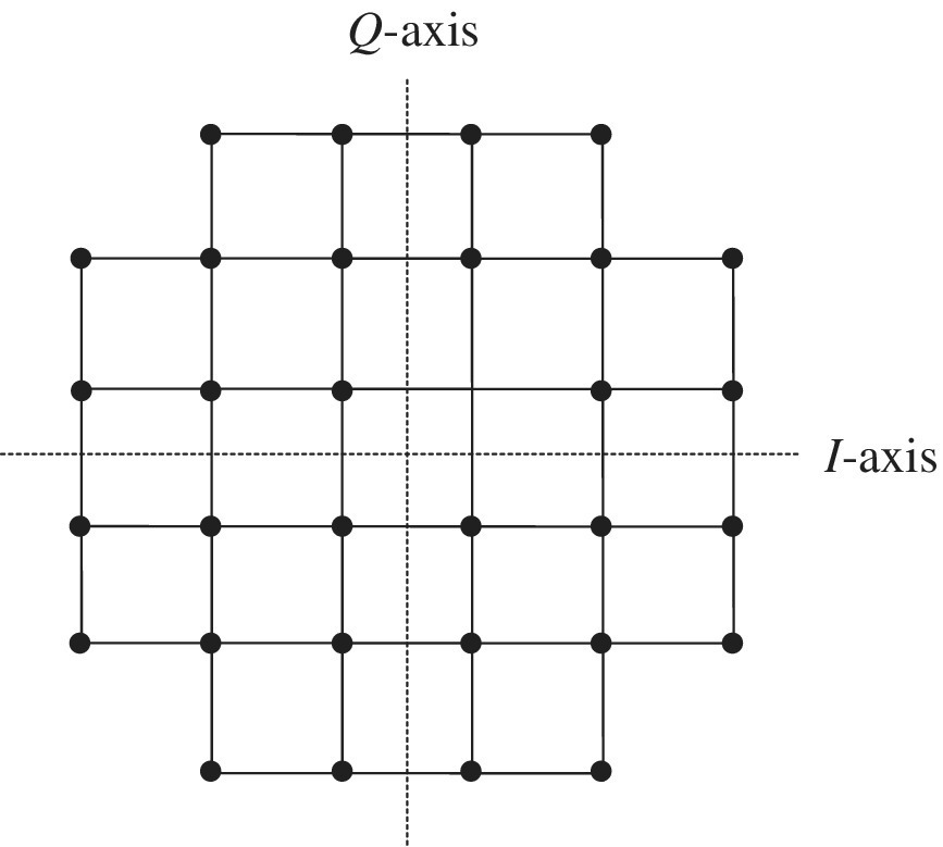
rest‐points expressed by (6.29), such that, MI = MQ = M resulting in a square constellation of rest‐points. On the other hand, when k′ is an odd integer there is no such underlying PAM constellation and the ![]() rest‐points αIm and αQm result in a rectangular or non‐square constellation. In this case, the constellation is selected to minimize the average power and peak‐to‐average power ratio. Example rest‐point constellations for these two cases are shown in Figures 6.11 and 6.12 for k′ = 3 and 4 corresponding to 8‐ary QAM and 16‐ary QAM, respectively; these constellations are shown with gray coded symbol assignment.
rest‐points αIm and αQm result in a rectangular or non‐square constellation. In this case, the constellation is selected to minimize the average power and peak‐to‐average power ratio. Example rest‐point constellations for these two cases are shown in Figures 6.11 and 6.12 for k′ = 3 and 4 corresponding to 8‐ary QAM and 16‐ary QAM, respectively; these constellations are shown with gray coded symbol assignment.

FIGURE 6.11 Rectangular constellation: 8‐ary QAM modulation (gray‐coded).

FIGURE 6.12 Square constellation: 16‐ary rectangular QAM modulation (gray‐coded).
The symbol‐error probability for the cases with k′ = even is readily obtained using (6.38) and (6.39) with ![]() and recognizing that the quadrature channel is independent and identically distributed with equal symbol‐error probability and average power so, considering both channels, the overall symbol‐error probability is evaluated as
and recognizing that the quadrature channel is independent and identically distributed with equal symbol‐error probability and average power so, considering both channels, the overall symbol‐error probability is evaluated as

where ![]() . Equation (6.42) is plotted as the solid curves in Figure 6.13 for M′ corresponding to k′ = even integer. With gray coding the approximate expression for the bit‐error probability, for sufficiently high values of Eb/No, is simply
. Equation (6.42) is plotted as the solid curves in Figure 6.13 for M′ corresponding to k′ = even integer. With gray coding the approximate expression for the bit‐error probability, for sufficiently high values of Eb/No, is simply ![]() .
.

FIGURE 6.13 Symbol‐error performance of M‐ary QAM modulation.
When k′ = odd integer the signal rest‐point constellation, shown in Figure 6.11 for k′ = 3, is not square, however, it can be formulated as a rectangular constellation with row‐column dimensions MI and MQ such that MI = 2MQ and MI MQ = M′. The symbol‐error probability is expresses as
where PIsc and PQsc are the probabilities of a correct symbol in the respective dimensions. Letting x = {I,Q}, these expressions for the correct symbol detection probability are evaluated as

Equation (6.43) is evaluated using (6.44), corresponding to the I and Q rails, and plotted as the dashed curves in Figure 6.13.
6.4 ALTERNATE QAM WAVEFORM CONSTELLATIONS
The performance for k′ = odd integers in Figure 6.13, that is, for M = 8, 32, 128, and 512, corresponds to the rectangular rest‐point constellations as shown in Figure 6.11 for 8‐ary QAM with k′ = 3. These constellations require a relatively high average power and the performance can be improved through a more judicious selection of the rest‐point locations. For example, the constellation in Figure 6.11 is re‐drawn in Figure 6.14 as two concentric circles with equal distances between the nearest neighbors. Because this constellation contains rest‐points on concentric circles, it is referred to as APSK modulation. Four sets of nearest neighbors result in two bit‐errors so gray coding is not fully achievable. On the other hand, if the outer circle constellation were rotated counterclockwise by 45°, gray coding is achievable; however, the outer radius circle must be decreased slightly to achieve the same distance between all of the rest‐points. It is left as an exercise (see Problems 8 and 9) to analyze the performance of this constellation and compare it with the performance of the phase‐shifted outer constellation with the adjusted radius to provide equal Euclidian distances between all adjacent rest‐points.

FIGURE 6.14 Concentric circular constellations: 8‐ary APSK modulation (partial gray coding).
6.5 CASE STUDY: 16‐ary QAM PERFORMANCE EVALUATION
This case study examines the performance of 16‐ary QAM using the rest‐point configuration shown in Figure 6.12. Referring to the functional demodulator implementation shown in Figure 6.15, the filtering and sample rate reduction provides four complex samples‐per‐symbol with a bandwidth of 2Rs Hz into the phase rotation and matched filtering functions. The fast AGC derives the signal level error in a bandwidth comparable to the input BPF bandwidth and is used during acquisition. The slow narrowband AGC is used to maintain the signal level throughout the data detection processing. The slow AGC, phaselock loop, and symbol timing errors are derived from the decision logic depicted in Figure 6.16; otherwise, these tracking functions operate in a conventional manner. The slow AGC error is computed as the magnitude difference between the rest‐point and matched filter vectors; the PLL phase error is the angle between the two vectors. The symbol timing error derivation is not explicitly shown, however, is derived from the difference between early and late samples of the matched filter output.

FIGURE 6.15 Functional implementation of an M‐ary QAM demodulator implementation.

FIGURE 6.16 QAM demodulator decision logic.
Figure 6.17 compares the simulated bit‐error performance as the circled data points and the corresponding theoretical gray‐code approximation from Figure 6.13. The dashed curve is the simulated symbol‐error performance that approaches 4 × Pbe as the signal‐to‐noise ratio increases. The Monte Carlo simulations are based on 1 M symbols for each signal‐to‐noise ratio and use ideal AGC, phase and symbol timing tacking.7 The transmitted signal uses the rect(t/T) symbol shaping function and the spectrum is shown in Figure 6.18. This traditional sinc(fT) frequency response, with first spectral sidelobe levels of −13 dB, can be improved with the use of spectral root‐raised‐cosine shaping as discussed in Sections 4.3.2, 4.4.1.1, and 4.4.4.1.

FIGURE 6.17 Simulated performance of 16‐ary QAM modulation (Figure 6.12, gray‐coded).

FIGURE 6.18 QAM signal spectrum (p(t) = rect(t/T)).
6.6 PARTIAL RESPONSE MODULATION
The following concepts dealing with partial response modulations are largely based on the ground breaking work of Nyquist [5, 6]. Partial response modulation is a form of multilevel pulse code modulation (PCM)8 or PAM in which intentional intersymbol interference is permitted to confine the power spectral density (PSD) of the transmitted signal. The resulting redundant modulation signal states conform to unique state transitions and transition violations are used to detect the presence of errors in the demodulation processing. Partial response is also referred to as correlative coding and was introduced by Lender [7] as duobinary modulation in which a data rate of twice that of conventional binary modulation is achieved with a narrower PSD bandwidth. The duobinary modulation is contrasted with Nyquist binary signaling as characterized in (6.45) and (6.46) using the Fourier transform relationship ![]() . These relationships and the following analysis ignore causality:
. These relationships and the following analysis ignore causality:


The frequency and time functions are plotted in Figure 6.19. Figure 6.19a depicts the uncorrelated spacing of the Nyquist impulse response at intervals of t = ±nT: n > 0. These intervals are contrasted with the duobinary uncorrelated intervals of t = ±(n + 1/2)T: n > 0 shown in Figure 6.19b. In both cases, the filled circles are separated by the symbol interval of T seconds and represent sampling instances of the input data. The duobinary filter response, at the sampling instances t = ±T/2, results in correlation between adjacent symbols in the sequence of input source data [8, 9]. The duobinary, or 119 partial response, correlative encoding depicted in Figure 6.19b is also referred to as polybinary and biternary coding.

FIGURE 6.19 Comparison of Nyquist and duobinary spectrums and impulse responses.
The only way that 2W bits/s can be transmitted through a channel with bandwidth W = Rb/2 without experiencing intersymbol interference is to use the Nyquist filter described by (6.45) and depicted in Figure 6.19a. However, the sharp cutoff frequency of this filter and the resulting infinitely long impulse response results in an unrealizable filter that requires time and frequency design compromises as discussed in Section 4.4.4.1. The characteristic of the ideal Nyquist filter, that results in no intersymbol interference, is the orthogonal spacing of the impulse response at instances of ±nT: |n| > 0 as depicted by the filled circles in Figure 6.19a. As shown in Figure 6.19b, orthogonal spacing also exists for duobinary modulation, however, the symbol responses occurring at t = ±0.5T both have unit amplitudes and result in intentional or known intersymbol interference between adjacent symbols. The cosine‐shaped frequency response of the duobinary‐modulated signal in confined to the same bandwidth as the Nyquist filter; however, the noise bandwidth is Bn = 1/4T Hz. The cosine frequency roll‐off also results in lower impulse response sidelobes and less sensitivity to channel impairments and demodulator frequency and timing errors compared to the Nyquist filter.
The duobinary baseband waveform modulation and demodulation using a random sequence of source data bits, denoted as bi = {0,1}, is shown in Figure 6.20. The bandwidth of the duobinary spectrum supports an information capacity of 2 bits/Hz by incorporating three distinct amplitude levels obtained by the correlative processing resulting from the known intersymbol interference as described above. For example, referring to Figure 6.20, the source data bits (bi) are modulo‐two added (⊕) to the previously encoded data Di−1 resulting in the differentially coded data Di = Di−1 ⊕ bi for i = 1, 2, …. The reference data D0 is set to 0 corresponding to space data. This coding prevents catastrophic error propagation when an error occurs in the channel. The three correlative encoded signal levels, constituting the duobinary waveform, are obtained by algebraically adding the differentially encoded data resulting in the modulated signal levels ℓi = Di + Di−1 indicated in Figure 6.20. The result is a three‐level modulated signal corresponding to ℓi = {0,1,2} as depicted in the third sequence in the figure.

FIGURE 6.20 Example of duobinary baseband modulation and demodulation.
The decoding of the received duobinary waveform is based on the detection threshold levels Ld1 and Ld2 that are established to correspond to the minimum distance dm = A/2(L − 1) between the L = 3 levels corresponding to ℓi = {0,1,2}.10 Based on this description, the demodulated data estimates ![]() = 1 correspond to the decisions ℓi = 1 and
= 1 correspond to the decisions ℓi = 1 and ![]() = 0 correspond to the decisions ℓi = 0 or 2. In general, for the correlative‐encoded data decisions as described above, mark and space data correspond, respectively, to odd and even values of ℓi; this is useful in decoding the multilevel correlative coding as described by Lender [10] and discussed in Section 6.6.1. This description of the duobinary modulator results in unipolar modulation levels corresponding to ℓi ≥ 0 is shown in Figure 6.21a. An alternate coding configuration, resulting in the bipolar modulation levels ℓi = {−2,0,2} is shown in Figure 6.21b.
= 0 correspond to the decisions ℓi = 0 or 2. In general, for the correlative‐encoded data decisions as described above, mark and space data correspond, respectively, to odd and even values of ℓi; this is useful in decoding the multilevel correlative coding as described by Lender [10] and discussed in Section 6.6.1. This description of the duobinary modulator results in unipolar modulation levels corresponding to ℓi ≥ 0 is shown in Figure 6.21a. An alternate coding configuration, resulting in the bipolar modulation levels ℓi = {−2,0,2} is shown in Figure 6.21b.

FIGURE 6.21 Encoding of duobinary baseband signal.
The correlative coded data in Figure 6.20 must be filtered to restrict the modulated signal spectrum. In keeping with the optimum detected filter in an AWGN channel, the duobinary filter is split between the modulator and demodulator filters expressed, respectively, as
where Hd(fTb) represents the demodulator matched filter. The correlative coded data are filtered as shown in Figure 6.22 that also includes the channel, demodulator matched filter, and data recovery processing. In this case, the unipolar differential encoder output is level coded corresponding to the unipolar‐to‐bipolar mapping {1,0} ≥ {1,−1}. The resulting bipolar sampled data jTs is then passed through the channel and the duobinary matched filter. For example, with Ns samples‐per‐symbol, the symbol counter i is derived from the sample counter j according to the condition11: if mod(j,Ns) = 0 then i is indexed by one, so, at the beginning of each symbol, a unit pulse 2Di − 1 of duration Ts is applied to the filter. As indicated in the figure, the remaining Ns − 1 samples for each symbol are input as zero. The filter weights ![]() : −N/2 ≤ n ≤ N/2 correspond to N + 1 symmetrical samples of the duobinary impulse response. The discrete samples are evaluated as
: −N/2 ≤ n ≤ N/2 correspond to N + 1 symmetrical samples of the duobinary impulse response. The discrete samples are evaluated as ![]() ⇔ Hm(m) where Hm(m) is the discrete‐sample characterization of the duobinary spectrum as expressed in (6.47).12 After passing the jTs samples through the channel and demodulator matched filter, the iT received data samples are processed as shown in Figure 6.2213 to determine the received bit estimates
⇔ Hm(m) where Hm(m) is the discrete‐sample characterization of the duobinary spectrum as expressed in (6.47).12 After passing the jTs samples through the channel and demodulator matched filter, the iT received data samples are processed as shown in Figure 6.2213 to determine the received bit estimates ![]() . Figure 6.23 shows the duobinary matched filter response, using the 30‐bit source data sequence: (111011001110000111010011010011) and a noise‐free channel. Upon examining the data recovery processing, it is seen that the recovered data estimates are identical to the source data, that is,
. Figure 6.23 shows the duobinary matched filter response, using the 30‐bit source data sequence: (111011001110000111010011010011) and a noise‐free channel. Upon examining the data recovery processing, it is seen that the recovered data estimates are identical to the source data, that is, ![]() = di. Using the magnitude of the matched filter samples eo(iT) simplifies the decision processing.
= di. Using the magnitude of the matched filter samples eo(iT) simplifies the decision processing.

FIGURE 6.22 Simplified implementation of duobinary baseband system.

FIGURE 6.23 Duobinary matched filter response and optimum detection samples.
Figure 6.24 shows the one‐to‐one correspondence between the sampled source data and the L = 3 levels of the demodulator matched filter sampled outputs. There is a one‐to‐one correspondence between the matched filter samples and the data samples such that the magnitude of the matched filter output maps into the optimally detected data estimates expressed as,


FIGURE 6.24 Duobinary sampled data and three‐level demodulator matched filter samples.
The bit‐error performance of the duobinary‐modulated signal is evaluated using the filtered bipolar coded detection levels as characterized in Figure 6.21b. Considering the AWGN channel, the decision regions are depicted in Figure 6.25 for the bipolar and bipolar‐magnitude detection processing.

FIGURE 6.25 Demodulator decision regions for duobinary waveform detection.
The probability distribution functions for the conditions indicated in Figure 6.25 are expressed as follows:

Using the a priori probabilities P0 and P1 and integrating the appropriate pdfs over the indicated ranges, the conditional probabilities, using the bipolar levels characterized in Figure 6.25a, are evaluated as

and

Performing the integrations in (6.50) and (6.51) and expressing the result in terms of the complement of the probability integral, the conditional probabilities simplify to

and

Based on (6.52) and (6.53), the total‐error probability is evaluated as

where ![]() is the baseband peak signal‐to‐noise ratio. Equation (6.54) is also obtained when the error probability is evaluated using the magnitude of the bipolar levels as characterized in Figure 6.25b. Forming the magnitude of the received bipolar waveform simplifies the detection processing since a matched filter detection below the single threshold of Ld = 1 is declared a mark bit (
is the baseband peak signal‐to‐noise ratio. Equation (6.54) is also obtained when the error probability is evaluated using the magnitude of the bipolar levels as characterized in Figure 6.25b. Forming the magnitude of the received bipolar waveform simplifies the detection processing since a matched filter detection below the single threshold of Ld = 1 is declared a mark bit (![]() = 1), otherwise, a space bit (
= 1), otherwise, a space bit (![]() = 0) is declared.
= 0) is declared.
The term involving the argument 9γ/4 has a negligible effect of the error probability. For example, when Pe is expressed in scientific notation the significand (mantissa) is altered in the third and fourth decimal place for 0 ≤ γb ≤ 20 dB where γb is the signal‐to‐noise ratio measured in the bandwidth equal to Rb. Consequently, indifference to current usage, the error probability is expressed as

The argument of the square‐root in (6.55) must be expressed in terms of the maximum signal‐to‐noise ratio, E/No, at the output of the demodulator matched filter, where E is the signal energy and No is the AWGN noise density. Since the preceding analysis involves the baseband characterization of the duobinary waveform, using the demodulator matched filter Hd(fT), defined by (6.47), and Parseval’s relationship, the duobinary symbol energy is expressed as

However, since Hd(fT) is real‐valued with ![]() , the integral involving H(fT) is expressed, in terms of the square‐root of the signal power at the matched filter output, as
, the integral involving H(fT) is expressed, in terms of the square‐root of the signal power at the matched filter output, as

Therefore, the average received signal power is ![]() and the corresponding symbol energy is
and the corresponding symbol energy is ![]() resulting in the error probability expressed as
resulting in the error probability expressed as

This result is reconciled with (6.55) by considering the definition of the argument given by

Substituting A2/2 given above and ![]() , where Tb is the bit interval corresponding to 1 bit/symbol, (6.59) is expressed as
, where Tb is the bit interval corresponding to 1 bit/symbol, (6.59) is expressed as

The second equality in (6.60) is based on the duobinary waveform corresponding to 2 bits/symbol or Tb = 2T. Consequently, the argument (γ/4) of the square‐root in (6.55) corresponds to that of the duobinary filtered result in (6.58). However, the duobinary spectrum in (6.46) has a lowpass bandwidth of ![]() corresponding to the Nyquist rate of
corresponding to the Nyquist rate of ![]() bits/channel‐use. Therefore, the interval T is the bit interval for the duobinary waveform so that
bits/channel‐use. Therefore, the interval T is the bit interval for the duobinary waveform so that ![]() and the equality in (6.60) applies to the duobinary bit‐error probability expressed as
and the equality in (6.60) applies to the duobinary bit‐error probability expressed as

where ![]() . Lucky, Salz, and Weldon [11] arrive at the same result using the signal distance d and the bit‐error probability expressed by (3.32).
. Lucky, Salz, and Weldon [11] arrive at the same result using the signal distance d and the bit‐error probability expressed by (3.32).
Equation (6.61) is plotted as the solid curve in Figure 6.26 as a function of γb in decibel. The theoretical bit‐error probability of unipolar non‐return to zero (NRZ) PCM coding is 3 dB worse than antipodal signaling and the duobinary performance is degraded by an additional −20log10(π/4) = 2.1 dB from that of unipolar NRZ PCM. The circled data points correspond to Monte Carlo simulation of the duobinary performance using 1M bits/signal‐to‐noise ratio for γb < 12 dB, otherwise 10M bits are used. The 2.1 dB loss in the duobinary performance can be reduced with maximum‐likelihood sequence estimation [12] (MLSE) detection over several bits using a trellis state decoder. Because of the correlation between adjacent bits, the demodulation processing of the 11 duobinary coded waveform provides for error detection by observing violations of the following rule: two consecutive space bits with an intervening even number of mark bits have opposite polarity, otherwise, if the intervening mark bits is odd the polarity of the space bits is the same.

FIGURE 6.26 Bit‐error performance of duobinary modulation.
6.6.1 Modified Duobinary Modulation
The modified duobinary response results in a −1 0 114 filter impulse response when sampled at the instances t = nT; n = −1,0,1; otherwise, the samples are all zero. The obvious difference between the modified duobinary and the 11 duobinary waveform is that the input signal samples are correlated with symbol samples separated by 2T instead of the adjacent symbol samples. However, as will be seen, the data corresponding to the modulated levels ℓi = 0 is di = 0 (space) and ℓi = ±2 is di = 1 (Mark). Another difference is that the transitions from a level can terminate on any of the levels so, unlike the 11 duobinary modulation, a transition from ℓi = −2 to ![]() = +2 may occur. Lender [10] points out that this large shift between levels reduces the horizontal eye opening, thus increasing the demodulator sensitivity to symbol timing errors and channel impairments. The modified duobinary waveform also uses three modulation levels with, as discussed in the preceding section,
= +2 may occur. Lender [10] points out that this large shift between levels reduces the horizontal eye opening, thus increasing the demodulator sensitivity to symbol timing errors and channel impairments. The modified duobinary waveform also uses three modulation levels with, as discussed in the preceding section, ![]() and provides 2 bits/channel‐use. At the optimum symbol sampling instances the vertical eye opening has zero intersymbol interference and the degradation in Eb/No with an AWGN channel is 2.1 dB. The −1 0 1 duobinary coded waveform provides for error detection by observing violations of the following rule: two consecutive mark bits with an intervening odd number of space bits have opposite polarity; otherwise, if the intervening space bits is even the polarity of the mark bits is the same. These claims are confirmed in the following analysis of the modified duobinary modulation.
and provides 2 bits/channel‐use. At the optimum symbol sampling instances the vertical eye opening has zero intersymbol interference and the degradation in Eb/No with an AWGN channel is 2.1 dB. The −1 0 1 duobinary coded waveform provides for error detection by observing violations of the following rule: two consecutive mark bits with an intervening odd number of space bits have opposite polarity; otherwise, if the intervening space bits is even the polarity of the mark bits is the same. These claims are confirmed in the following analysis of the modified duobinary modulation.
The modified duobinary filter and the corresponding impulse response are described by (6.62). These respective functions are plotted in Figure 6.27 in terms of the normalizing parameter T.


FIGURE 6.27 Modified duobinary spectrum and impulse response.
The frequency response is a sine function contained within the Nyquist band W = Rb/2 providing 2W = Rb bits/s or 2 bits/symbol or channel use. As with the duobinary cosine filter, the sine filter results in controlled intersymbol interference; however, in this case the non‐zero filter impulse responses occur at t/T = ±1 with a correlation interval of 2T resulting in the notation –1 0 1 partial response.15 Differential coding of the source data (Di), the unipolar‐to‐bipolar translation (Bi), and level coding (ℓi) are defined for a source sequence of unipolar binary unipolar non‐return to zero level (NRZ‐L) data di: i = 1, 2, … as follows:

where the two differentially coded bits are defined as D−1 = D0 = 0. With Bi = {±1}, the number of coded levels ℓ is L = 3. The correspondence of the coded levels with the source bits and the criteria for detecting demodulator bit‐error conditions is verified by examining the coding using the defined sequence of data (see Problem 15). The bit‐error probability performance loss of the modified duobinary modulation, under ideal channel and demodulator timing conditions, is 2.1 dB. This loss is established by examining the symbol energy of the modified duobinary modulation (see Problem 20).
The property of the modified duobinary filter corresponding to a zero direct current (DC) component, that is, H(0) = 0, is significant, in that, this is a necessary requirement for the generation of a single‐sideband (SSB) modulated waveform. The SSB waveform is obtained by passing h(t) through a Hilbert filter [13, 14], forming ![]() , with the SSB baseband waveform informally expressed as
, with the SSB baseband waveform informally expressed as
where di is the information data.
6.6.2 Multilevel Duobinary Modulation
The multiple levels, exceeding L = 3 discussed in the preceding section, can be applied to the duobinary, modified duobinary, and other partial response modulations involving higher order filter functions mentioned in the following section. The inclusion of additional modulation levels results in the information capacity expressed as
where n = L − 1 is the span of the filter correlation interval.16 The PSD is concentrated in an increasingly narrow bandwidth by virtue of a filter correlation length spanning n symbols. The multilevel duobinary frequency function is expressed as

The filter frequency function is plotted in Figure 6.28 for values of L = 3 through 7 with the dashed curve corresponding to the cosine filter in Figure 6.19b. The corresponding impulse responses are left as an exercise (see Problem 20); however, the filter impulse response exhibits n unit‐amplitude levels occurring at t/T, such that, for i = 0, …, n − 1, t/T is expressed as


FIGURE 6.28 Multilevel duobinary spectrum.
The unit‐amplitude samples are symmetrical about t/T = 0 with zero sample values at all other values of i.
The modulator encoding of the multilevel duobinary waveform is similar to that of the three‐level waveform; however, the differential encoding spans n bits including the current source bit di: i = 1, 2, … and the n − 1 previously differentially encoded bits Di−m: m = 1, …, n − 1. The parameters D–m = 0: m = n − 1, …, 0 are initialized as space bits and the corresponding parameters B−m are initialized as B−m = 2D−m − 1. With these normalizations, the encoding in (6.63) is generalized as

The coding described in (6.68) is depicted in Figure 6.29, under noise‐free conditions, for L = 4 levels (n = 3 correlated symbols) corresponding to 11117 duobinary modulation. The source data are represented by the square data samples with the circles representing the demodulator matched filter samples. As in the preceding duobinary examples, there is a one‐to‐one correspondence between the matched filter sample and the received data; however, the mapping is not as straightforward as in the three‐level duobinary case expressed in (6.48). This PAM waveform can be implemented as a QAM waveform by applying differential encoding between the inphase and quadrature rails as discussed in Section 8.4.

FIGURE 6.29 Duobinary sampled data and four‐level demodulator matched filter samples.
The detection levels for L = 4 shown in Figure 6.29 are symmetrical about zero; however, there is no optimum sample at ℓ = 0 as in the L = 3 level duobinary case. The optimally sampled duobinary coding levels ℓ are shown in Table 6.1 for the indicated range of L.
TABLE 6.1 Comparison of Duobinary Coding Levels ℓ and Data d for 3 ≤ L ≤ 7
| Levels (L) | Coding | Levels/Data | ℓmax = n = L − 1 | ||||||
| 3 | 2 | 0 | −2 | ℓ | 2 | ||||
| 0 | 1 | 0 | d | ||||||
| 4 | 3 | 1 | — | −1 | −3 | ℓ | 3 | ||
| 1 | 0 | — | 1 | 0 | d | ||||
| 5 | 4 | 2 | 0 | −2 | −4 | ℓ | 4 | ||
| 0 | 1 | 0 | 1 | 0 | d | ||||
| 6 | 5 | 3 | 1 | — | −1 | −3 | −5 | ℓ | 5 |
| 1 | 0 | 1 | — | 0 | 1 | 0 | d | ||
| 7 | 6 | 4 | 2 | 0 | −2 | −4 | −6 | ℓ | 6 |
| 0 | 1 | 0 | 1 | 0 | 1 | 0 | d | ||
The conditions for the decoding of the data dj corresponding to the levels ℓj are given in Table 6.1. The distance between the levels is two and when mod(ℓmax/2,2) = 1 the optimally sampled matched filter levels are odd integer values symmetrical about zero. The binary data corresponding to negative levels are inverted with dj(ℓj > 0) = mod(dj (ℓj < 0),2). For the case mod(ℓmax/2,2) = 0, dj(ℓj > 0) = dj(ℓj < 0); however, when L is odd the level ℓ0 = 0 corresponds to d0 = 0, otherwise d0 = 1. Recognizing that the data dj(![]() ) = 0 ∀ L, the following procedure outlines the decoding decisions.
) = 0 ∀ L, the following procedure outlines the decoding decisions.
! ℓr is real-valued matched filter optimum sample.! ℓerr is real-valued error used for matched filter gain control.! ℓ, ℓmax, L, and icnt are integer-valuesℓmax = L – 1; icnt = 0lp do ℓ =, ℓmax, 2
if (ℓr >= real(ℓmax ‐1)) then; ℓerr =ℓr – real(ℓ)
else if(ℓr <real(ℓ- 1)) then; ℓerr =ℓr – real(ℓ)
exit lpendificnt = mod(icnt + 1,2)enddo lp
The decision level errors ℓerr are passed through a lowpass filter and applied to the matched filter gain control to ensure that the optimum decision levels are maintained for the duobinary demodulation. In the above examples, the optimum levels are defined in Table 6.1. In a simulation program or hardware test setup, the bit‐error probability is computed as the number of bit‐errors, ![]() , divided by the total number of received bits.
, divided by the total number of received bits.
6.6.3 Multilevel Duobinary Bit‐Error Performance
The bit‐error performance of multilevel duobinary modulation is expressed as [15]

Equation (6.69) is plotted in Figure 6.30 for the indicated values of L and the performance is summarized in Table 6.2.

FIGURE 6.30 Multilevel duobinary bit‐error performance.
TABLE 6.2 Summary of Multilevel Duobinary Performance
| Levels (L) | n | Loss* γb (dB) | γb (dB)* (Pbe = 10−5) | Capacity Rb/W bits/Use |
| 3 | 2 | 2.1 | 14.9 | 2.0 |
| 4 | 3 | 6.4 | 19.2 | 3.2 |
| 5 | 4 | 9.1 | 22.0 | 4.0 |
| 6 | 5 | 11.1 | 24.0 | 4.6 |
| 7 | 6 | 12.8 | 25.7 | 5.2 |
| 8 | 7 | 14.1 | 27.0 | 5.6 |
| 9 | 8 | 15.3 | 28.2 | 6.0 |
| 17 | 16 | 21.4 | 34.3 | 8.0 |
*Values from Figure 6.30.
6.6.4 Multilevel Duobinary Modulation using k‐bit Symbols
In this section, the multilevel duobinary‐modulated waveform is described by assigning k gray‐coded source bits to an M‐ary symbol and performing the duobinary coding described above to the source symbols. In this case, di represents the gray‐coded source bits and the duobinary coding is expressed in (6.70). The number of demodulator coded levels is L = 2M − 1 where M = 2k. This description of the duobinary‐modulated symbols results in a PAM waveform; however, the results can also be applied to the inphase and quadrature rails resulting in a QAM waveform. These concepts involving correlative coding have also been applied to frequency shift keying (FSK) and M‐ary phase shift keying (PSK) waveform modulations resulting in improved spectral containment [16–18].

An example of the duobinary symbol coding using k = 2 bits/symbol is given in Table 6.3. The previously defined 30‐bit binary example data sequence is used with the bits representing the gray‐coded source bits. The transmit data and the resulting demodulator matched filter sampled levels ℓi are shown, respectively, in Figure 6.31 as the square and circled sampled data points connected by the respective solid and dashed lines.
TABLE 6.3 Example of Duobinary Symbol Coding (k = 2 bits/symbol)
| Function | Ref. Data | Duobinary Coded Data | |||||||||||||||
| Gray‐coded bits (di) | 00 | 00 | 11 | 10 | 11 | 00 | 11 | 10 | 00 | 01 | 11 | 01 | 00 | 11 | 01 | 00 | 11 |
| Source symbols (si) | 0 | 0 | 3 | 2 | 3 | 0 | 3 | 2 | 0 | 1 | 3 | 1 | 0 | 3 | 1 | 0 | 3 |
| Differential coding (Di) | 0 | 0 | 3 | 3 | 0 | 0 | 3 | 3 | 1 | 0 | 3 | 2 | 2 | 1 | 0 | 0 | 3 |
| Bipolar conversion (Bi) | −3 | −3 | 3 | 3 | −3 | −3 | 3 | 3 | −1 | −3 | 3 | 1 | 1 | −1 | −3 | −3 | 3 |
| Level coding (ℓi) | 0 | 6 | 0 | −6 | 0 | 6 | 2 | −4 | 0 | 4 | 2 | 0 | −4 | −6 | 0 | ||
| Differential decode (s^i) | 3 | 2 | 3 | 0 | 3 | 2 | 0 | 1 | 3 | 1 | 0 | 3 | 1 | 0 | 3 | ||
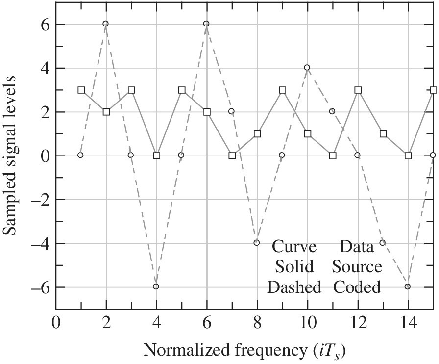
FIGURE 6.31 Example of multilevel duobinary coded symbols (k = 2 bits/symbol).
6.6.5 Classification of Partial Response Filters
Kretzmer [19, 20] expands the duobinary modulation of Lender by generalizing the implementation of partial response‐modulated waveforms. For example, the duobinary and the multilevel duobinary waveforms are categorized as Class 1 partial response waveforms, characterized by equal‐amplitude filter impulses. Class 2 partial response implementations result in a symmetrical triangular‐weighted set of filter impulses. The simplest case of the Class 2 partial response is the raised‐cosine Nyquist filter with α = 1 corresponding to the frequency and impulse responses expressed in (6.71) and shown in Figure 6.32. Although the frequency response extends over the range | f | ≤ W, the Nyquist criterion is satisfied resulting in impulses separated by T with zero responses otherwise as depicted by the filled circles in Figure 6.32. The triangular weighting results in a smoother, or more continuous, frequency response with much lower impulse response time sidelobes compared to those in Figure 6.19. This characteristic results in less sensitivity to demodulator symbol timing errors.


FIGURE 6.32 Class 2, n = 3 (1/2, 1, 1/2) partial response.
The Class 3 partial response, defined by Kretzmer, contains positive and negative impulse response components resulting from the ringing of the transient responses. The filters are characterized as causal lowpass filters, with a finite DC component, and result in nonsymmetrical decaying impulse components for t/T ≥ 0. The number of impulses is chosen by truncating the impulse response. Classes 4 and 5 are quasi bandpass filters with a zero DC component. The modified duobinary waveform discussed in Section 6.6.1 is a Class 4 partial response waveform; the Class 5 is similar, however, the frequency response corresponds to a sine‐squared function. For the classes of partial response considered, the best tolerance to signaling rate and channel impairments corresponds to the minimum value of n in each class.
ACRONYMS
- AGC
- Automatic gain control
- APSK
- Amplitude PSK
- ASK
- Amplitude shift keying
- AWGN
- Additive white Gaussian noise (channel)
- BPSK
- Binary phase shift keying
- DC
- Direct current
- FSK
- Frequency shift keying
- I/Q
- Inphase and quadrature (channels or rails)
- MLSE
- Maximum likelihood sequence estimation
- NRZ
- Non‐return to zero (PCM code format)
- NRZ‐L
- Non‐return to zero level (PCM code format)
- OOK
- On–off keying
- PA
- Power amplifier
- PAM
- Pulse amplitude modulation
- PCM
- Pulse code modulation
- PLL
- Phaselock loop
- PSD
- Power spectral density
- PSK
- Phase shift keying
- QAM
- Quadrature amplitude modulation
- QPSK
- Quadrature phase shift keying
- RF
- Radio frequency
- SSB
- Single‐sideband (modulation)
PROBLEMS
- Using (6.18) for the expressions of Pbe(Th) for coherent detection of OOK, derive the optimum detection threshold Tho that results in the minimum bit‐error probability.
Hint: Differentiate Pbe(Th) with respect to Th using the second equality in (6.18) and Leibniz’s Theorem and set the result equal to zero and solve for Tho. - Derive the optimum bit‐error probability (Pbe) for the coherent detection of OOK by substituting the optimum detection threshold Tho into the expression (6.18) for Pbe(Th). That is, show all of the steps used to arrive at
 in (6.19).
 - Consider the performance of a special case of OOK in which the space level is not zero but a small value given by α0 = ρα1 where 0 ≤ ρ ≤ 1. This situation was encountered in practice and resulted from a modulator implementation issue involving an analog amplifier bias. Derive the expression for the signal distance and the bit‐error probability and comment on the detection loss relative to the ideal OOK modulator.
- Repeat Problem 1 and find the optimum threshold for the noncoherent detection of OOK using the second equality in (6.22); the same hint applies.
- Repeat Problem 2 for the bit‐error probability of noncoherent detection of OOK by substituting the optimum threshold found in Problem 4 into (6.22).
- Derive general expressions in terms of M′ for the following QAM parameters for k′ = even and odd.
- The average signal power.
- The peak‐to‐average signal power ratio.
- Rewrite (6.42) in terms of the complementary error function erfc(x) and Eb/No.
- Derive the expression for the symbol‐error probability for the APSK modulation shown in Figure 6.14. Also, determine the average signal power and the peak‐to‐average power ratio.
- Determine the outer radius required to provide equal Euclidian distances between all nearest neighbors when the inner constellation in Figure 6.14 is rotated 45° clockwise as shown. Derive the expression for the symbol‐error probability for the modified APSK constellation. Also, determine the resulting average signal power and the peak‐to‐average power ratio. Do the 3‐bit eight symbol assignments result in gray coding?
- The rectangular constellation for the 32‐ary QAM waveform with k′ = 5 and symbol‐error probability shown in Figure 6.13, uses eight (8) I‐axis and four (4) Q‐axis rest‐points located symmetrically about the respective axes with a normalized minimum Euclidian distance of two between neighboring rest‐points. Reconfigure the 32‐ary constellation as shown below using the same Euclidian distances and compute the average power and the peak‐to‐average power ratio. Compute the same parameters for the 8 × 4 constellation and compare the results.
- Derive the expressions for the symbol‐error probabilities for the following 8‐ary QAM constellations when all neighboring rest‐points are separated by a normalized minimum distance of two. Compute the corresponding average power and the peak‐to‐average power ratio. Associate the eight 3‐bit symbols with the rest‐points to minimize the bit‐errors when a symbol error occurs. Is gray‐coding possible?

- Show all of the steps in the determination of the noise bandwidth of the duobinary spectrum expressed in (6.46).
- Show all of the steps in the evaluation of the inverse Fourier transform of the frequency function H(f) in (6.46) and confirm the corresponding impulse response.
- Using the probability density distribution p(y) and the random variable transformation y = |x|, where the random variable x is characterized as the normal distribution N(A, σx) and A is the level of bipolar NRZ‐L data sequence, show that the total‐error probability (Pe) is the same as expressed in (6.54).
Hint: Use the decision regions in Figure 6.25b and modifications to the corresponding pdfs in (6.49) based on the magnitude transformation. The final result is obtained by evaluating the conditional probabilities Pr(error|b = 0) and Pr(error|b = 1), performing the integrations over the range 0 ≤ y ≤ A/2, and computing Pe as the total‐error probability. - With the same source data sequence used in Figure 6.23, show the corresponding coded sequences Di, Bi, and ℓi using the modified duobinary‐modulated waveform. Compare the results with each of the related introductory comments in Section 6.6.1. The source sequence is: di = (11101100111000011101001101001).
- Using the same Bi sequence in Problem 15, determine the sequence
 based on the 10 −1 modified duobinary filter impulse response. As an alternative to determining the bit‐by‐bit sequence
  , simply show the relationship between
  and ℓi.
 - Evaluate the optimum samples of the received duobinary (L = 3) response to the binary source data sequence: 1010101010101010. Repeat the evaluation for the multilevel duobinary response using L = 4, and 5. Discuss how the received modulated sequence might be used and sketch a functional implementation of your idea(s).
- Determine the noise bandwidth of the modified duobinary‐modulated waveform.
- Show all of the steps in the evaluation of the inverse Fourier transform of the frequency function in (6.62) and confirm the corresponding impulse response.
- Using the multilevel filter function expressed in (6.66) evaluate and plot (or sketch) the impulse response for n = 4 − 7.
REFERENCES
- 1. J.I. Marcum, “A Statistical Theory of Target Detection by Pulsed Radars,” RAND Research Memorandum, RM‐754, RAND Corporation, Santa Monica, CA, December 1, 1947.
- 2. J.I. Marcum, P. Swerling, “Studies of Target Detection by Pulsed Radar,” IRE Transactions on Information Theory, Vol. IT‐6, No. 2, Special Monograph Issue, April 1960.
- 3. J.I. Marcum, “Table of Q Functions,” RAND Research Memorandum, RM‐339, RAND Corporation, Santa Monica, CA, January 1, 1950.
- 4. D.E. Johansen, “New Techniques for Machine Computation of the Q‐Function, Truncated Normal Deviates and Matrix Eigenvalues,” Applied Research Laboratory, Sylvania Electronic Systems, Scientific Report No. 2, Waltham, MA, July 1961.
- 5. H. Nyquist, “Certain Factors Affecting Telegraph Speed,” Bell System Technical Journal, Vol. 3, No. 2, pp. 324–346, April 1924.
- 6. H. Nyquist, “Certain Topics of Telegraph Transmission Theory,” Proceedings of the IEEE, Vol. 90, No. 2, pp. 280–305, February 2002. This paper was first published in the Transaction of the AIEE, Vol. 47, No. 2, pp. 617–644, April 1928.
- 7. A. Lender, “The Duobinary Technique for High‐Speed Data Transmission,” AIEE Transactions of the Communication and Electronics, Vol. 82, No. 2, pp. 214–218, May 1963.
- 8. A. Lender, “Correlative Digital Communications Techniques,” IEEE Transactions Communication Technology, Vol. 12, No. 4, pp. 128–135, December 1964.
- 9. A. Lender, Digital Communications: Microwave Applications, Chapter 7, K. Feher, Editor, “Correlative (Partial Response) Techniques and Applications to Digital Radio Systems,” Prentice‐Hall, Inc., Englewood Cliffs, NJ, 1981.
- 10. A. Lender, “Correlative Level Coding for Binary‐Data Transmission,” IEEE Spectrum, Vol. 3, No. 2, pp. 104–115, February 1966.
- 11. R.W. Lucky, J. Salz, E.J. Weldon, Jr., Principles of Data Communication, Chapter 4, “Baseband Pulse Transmission,” pp. x83–92, McGraw‐Hill, New York, 1968.
- 12. J.G. Proakis, “Maximum‐Likelihood Sequence Estimation of Digital Signals Transmitted over Time‐Dispersive Channels,” Department of Electrical Engineering, Northeastern University, Boston, MA, August 1976.
- 13. F.K. Becker, E.R. Kretzmer, J.R. Sheehan, “A New Signal Format for Efficient Data Transmission,” Bell System Technical Journal, Vol. 45, No. 5, pp. 755–758, May–June 1966.
- 14. R.W. Lucky, J. Salz, E.J. Weldon, Jr., Principles of Data Communication, Chapter 7, “Linear Modulation Systems,” pp. 197–199, McGraw‐Hill, New York, 1968.
- 15. R.W. Lucky, J. Salz, E.J. Weldon, Jr., Principles of Data Communication, Chapter 4, “Baseband Pulse Transmission,” pp. 88–90, McGraw‐Hill, New York, 1968.
- 16. D. Roth, “Mean Power Density Spectrum of a Continuous FSK Signal Modulated by the Duobinary Sequence,” National Telecommunications Conference, NTC74, pp. 572–589, San Diego, CA, 1974.
- 17. W.J. Melvin, R.W. Middlestead, “Power Density Spectrum of M‐ary Correlative Encoded MSK,” International Conference on Communications, ICC77, pp. 3.6.60–3.7.63, Chicago, IL, 1977.
- 18. G.S. Deshpande, P.H. Wittke, “The Spectrum of Correlative Encoded FSK,” International Conference on Communications, ICC78, pp. 25.3.1–25.3.5, Toronto, Ontario, 1978.
- 19. E.R. Kretzmer, “Binary Data Communication by Partial Response Transmission,” IEEE Annual Communication Convention, Conference Record, pp. 451–455, Boulder, CO, 1965.
- 20. E.R. Kretzmer, “Generalization of a Technique for Binary Data Communication,” IEEE Transactions on Communication Technology, Vol. 14, No. 1, pp. 67–68, February 1966.