
8
CODING FOR IMPROVED COMMUNICATIONS
8.1 INTRODUCTION
Before delving into the details of error detection and forward error correction (FEC) techniques, it is useful to describe several baseband coding techniques. In the following sections, various forms of baseband pulse code modulation (PCM) are discussed. PCM codes and data compression codes are source coding techniques. Following the description of PCM waveforms, a variety of important coding‐related topics are introduced: gray coding1 in Section 8.3 and differential coding in Section 8.4; pseudo‐random noise (PRN) sequences in Section 8.5; binary cyclic codes in Section 8.6; cyclic redundancy check (CRC) codes in Section 8.7; data randomizing, or scrambling in Section 8.8; data interleaving in Section 8.9. Following these topics, several forms of FEC channel coding are discussed; Wagner coding and decoding in Section 8.10; convolutional coding and Viterbi decoding in Section 8.11; turbo codes (TCs), parallel concatenated convolutional codes (CCCs) (PCCCs), serially CCCs (SCCCs), double parallel CCCs (DPCCCs), and double serially CCCs (DSCCCs) with reference to the related hybrid CCCs (HCCCs), and self‐concatenated codes (SCCs) in Section 8.122 (the nonturbo codes are collectively referred to as turbo‐like codes); low‐density parity‐check (LDPC) codes, product codes (PCs), and turbo product codes (TPCs) are introduced in Section 8.13; and Bose–Chaudhuri–Hocquenghem (BCH) codes, including M‐ary Reed–Solomon (RS) codes and RS Viterbi (RSV) codes, are discussed in Section 8.14.
The subject of coding to improve the performance of communication systems is broad and, in certain instances, requires knowledge in specialized areas like matrix and Boolean algebra and the theory of groups, rings, and fields. For example, an understanding of polynomials in the Galois field (GF) is crucial in the coding and decoding of both block and cyclic codes. These disciplines will be engaged only to the extent that they can be applied in a practical way to the coding and decoding of the various techniques considered. Several coding techniques are listed in Figure 8.1.

FIGURE 8.1 Channel coding techniques.
8.2 PULSE CODE MODULATION
Baseband signals are characterized as those signals with the signal energy concentrated around zero frequency, although the zero‐frequency power spectral density, S(f = 0), may be zero. This is contrasted to bandpass signals that are associated with a carrier frequency around which the signal energy is concentrated. The data from an information source is typically formatted as binary data with a mark bit representing logic 1 and space bit representing logic 0 data. In cases involving analog information sources, the information is time‐sampled and amplitude‐quantized and represented as binary data. In either event, the resulting binary data can be represented as a form of PCM [2] that contains all of the source information. The binary formatted data is typically denoted as a series of pulses, or bits, of duration Tb with amplitude levels of 1 and 0. A series of data defined in this manner is referred to as unipolar non‐return‐to‐zero (NRZ) formatted data [3], and with the binary amplitude levels of 1 and −1 the data format is referred to as polar NRZ. These and other baseband data formats are the subject of this section. There are a number of PCM codes that have been devised to address issues unique to certain applications; however, the most significant characteristics of the PCM codes are the power spectral density (PSD), bit synchronization properties, and the bit‐error performance. Other important characteristics involve the error detection and correction (EDAC) capabilities; however, the more powerful techniques in this regard use redundancy through increased bandwidth or decision space. A review of 25 baseband PCM codes and their properties is presented by Deffebach and Frost [4] and much of this section is based on their work. Another treatment of this subject is given by Stallings [5].
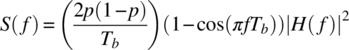
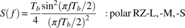
The PSD, with units of watt‐seconds/Hz, of binary PCM modulated random data sequences, with mark and space probabilities given by p and 1 − p, respectively, is evaluated by Bennett [6], Titsworth and Welch [7], and Lindsey and Simon [8] as

where Tb is the bit interval and Hm(f) and Hs(f) are the underlying spectrums of the mark and space bits. With unipolar formatted data, the mark data spectrum is defined as ![]() and the space data spectrum is zero, that is,
and the space data spectrum is zero, that is, ![]() , and upon substituting these results into (8.1) yields the unipolar PSD
, and upon substituting these results into (8.1) yields the unipolar PSD

With polar formatted data the space data spectrum is defined as ![]() so the polar PSD is given by
so the polar PSD is given by

These results are applied in the followings sections to evaluate the spectrums of various forms of unipolar and polar formatted PCM waveforms. Houts and Green [9] compare the spectral bandwidth utilization in terms of the percent of total power in bandwidths of {0.5,1,2,3}Rb for a variety of binary baseband coded waveform. In Section 8.2.5, the PCM demodulator bit‐error performance is examined.
8.2.1 NRZ Coded PCM
The designation NRZ denotes the binary format that characterizes a mark bit as being one amplitude level and space bit as another. When the space bit is represented by a zero level, the format is called unipolar NRZ. In contrast, when the level of the space bit is the negative of the mark bit level, the designation polar NRZ is used. The designation NRZ‐L indicates that the level of the binary format is changed whenever the level of the source data changes. These two PCM data formats are shown in Figure 8.2. The bipolar NRZ‐L format is a special tri‐level code for which a space source bit corresponds to a zero output level, while the level corresponding to the mark source data is bipolar, alternating between plus and minus levels.

FIGURE 8.2 Unipolar, polar, and bipolar NRZ‐L formatted data.
The designation NRZ‐M (NRZ‐S) indicates that changes in the formatted data occur when the source data is a mark (space); otherwise, the coded level remains the same. The unipolar NRZ‐M and NRZ‐S coded waveforms are depicted in Figure 8.3. This baseband coding results in differentially encoded data and is discussed in more detail in Section 8.4.

FIGURE 8.3 Unipolar NRZ‐M,‐S formatted data.
The advantage of differentially encoded data is that correct bit detection is maintained in the demodulator with a 180° error in the carrier phase as might occur in the channel or the demodulator carrier tracking loops. The penalty for using differential data coding is a degradation of the bit‐error performance with a 2 : 1 increase in the bit errors at high signal‐to‐noise ratios. Because the source data is encoded in the transitions of the PCM coded data, the absolute level is not as important; however, polar NRZ data with binary phase shift keying (BPSK) modulation results in the optimum detection performance through an additive white Gaussian noise (AWGN) channel.
The PSD of the unipolar NRZ level, mark, space NRZ‐L,‐M,‐S formatted data is evaluated using (8.2) with the underlying spectrum characterized by the unit amplitude pulse rect(t/Tb − 1/2) with the square of the spectrum magnitude expressed as

The sampled spectrum expressed by (8.4) results in zero magnitude at ![]() for all n except n = 0, in which case, the magnitude is
for all n except n = 0, in which case, the magnitude is ![]() . With random source data, corresponding to p = 1/2, (8.2) becomes
. With random source data, corresponding to p = 1/2, (8.2) becomes

The PSD for the polar NRZ coded waveform is evaluated in a similar way using (8.3) and (8.4) and, assuming random data with p = 1/2, the result is

Therefore, the polar NRZ coded waveform has 6 dB more energy in the underlying spectrum, and there is no zero‐frequency impulse.
The spectrum for the bipolar NRZ‐L,‐M,‐S is evaluated by Sunde [10] as
The PSD in (8.4) is based on the PCM coded data having a constant amplitude over the entire bit interval, that is, the there is no pulse shaping, and, assuming random source data with p = 1/2, upon substituting |H(f)|2 using (8.4) into (8.7) yields the PSD for bipolar NRZ coded PCM expressed as

Equations (8.5), (8.6), and (8.8) are normalized by Tb and plotted in Figure 8.4 as the PSD for the NRZ coded PCM waveforms. The spectrum of the bipolar NRZ code does not have a direct current (DC) component so transmission over lines that are not DC coupled is possible as, for example, over long‐distance lines that use repeater amplifiers.

FIGURE 8.4 Power spectral density for NRZ coded PCM waveforms.
8.2.2 Return‐to‐Zero Coded PCM
Another form of baseband coding is return‐to‐zero (RZ) coding that is characterized by the NRZ‐L coding in Figure 8.2 with the exception that the bit interval is split, that is, the coded pulse level is nonzero over the first Tb/2 data interval and returns to zero over the remaining interval.3 The RZ coded PCM waveforms are depicted in Figure 8.5. In the unipolar case, the space bit is always zero and the mark bit is split. The polar case is similar; however, the space bit is split with the opposite polarity of the mark bit. The polar RZ code allows the bit timing to be established simply by full‐wave rectifying and narrowband filtering the received bit stream.

FIGURE 8.5 RZ formatted data.
In the bipolar case, the mark bit is split with alternating polarities and the space bit is always zero. By alternating the polarity of the mark bits, the bipolar RZ code provides for one bit‐error detection [11]. The bipolar RZ coded PCM is used in the Bell Telephone T1‐carrier system [12].
The PSD of the unipolar and polar RZ coded PCM waveforms are evaluated using (8.2) and (8.3) in a manner similar to that used for the unipolar and polar NRZ code; however, in these cases, the mark bit is split and characterized by the pulse rect(2t/Tb − 1/2) with the underlying square of the spectrum magnitude given by

Substituting (8.9) into (8.2) and recognizing that the spectrum is zero for all n ≠ 0, the PSD of the unipolar RZ coded waveform with random data is evaluated as

In a similar manner, the polar RZ PSD is evaluated using (8.3) with the result
The PSD of the bipolar RZ coded PCM waveform is characterized by Sunde [10] as in (8.7), with ![]() given by (8.9) so that, with random data,
given by (8.9) so that, with random data,

The PSD of the bipolar RZ coded PCM waveform is plotted in Figure 8.6.

FIGURE 8.6 Power spectral density for RZ coded PCM waveforms.
8.2.3 Biphase (Biϕ) or Manchester Coded PCM
Biphase (Biϕ), or Manchester, coded PCM is a commonly used waveform because of the robust bit timing recovery even without random data. For example, in an idle mode that uses either mark or space hold data, the demodulator timing can be maintained. The biphase‐level, ‐mark, ‐space (Biϕ‐L,‐M,‐S) coded waveforms are depicted in Figure 8.7. For the Biϕ‐L code, the mark bit is split and the space bit is the inverse of the mark bit. With the Biφ‐M code, a transition occurs at the beginning of each source data bit and the mark bit is split; however there is no change in the code‐bit level when a space source bit occurs. The Biϕ‐S code is similar to the Biϕ‐M with the role of the mark and space bits reversed.

FIGURE 8.7 Biphase Biϕ‐L,‐M,‐S polar formatted data.
The PSD of the biphase coded PCM waveform, using random data with p = 1/2, is evaluated by Batson [13] as

Equation (8.13) is normalized by Tb and plotted in Figure 8.8.

FIGURE 8.8 Power spectral density for Biϕ‐L,‐M,‐S coded PCM waveforms.
8.2.4 Delay Modulation or Miller Coded PCM
Delay modulation (DM), or Miller code, is a form of PCM where, for DM‐M coding, the code bit corresponding to each mark source bit is split, that is, the level changes in middle of each mark bit. The level of the code bit corresponding to a space source bit is unchanged unless it is followed by another space source bit in which case it is changed at the beginning of the space source bit. The DM‐S coding reverses the roles of the mark and space source bits, that is, the code bit corresponding to each space source bit is split and the level of the code bit corresponding to a mark source bit is unchanged unless it is followed by another mark source bit in which case it is changed at the beginning of the mark source bit. DM‐M,‐S coding is shown in Figure 8.9 for the source data sequence (1,0,0,1,1,0,1). To establish the correct phase of the bit timing in the demodulator an alternating mark‐space preamble must be transmitted.

FIGURE 8.9 Delay Modulation DM‐M,S coded PCM waveforms.
The PSD of the DM coded PCM waveform is evaluated for random data by Hecht and Guida [14] as

Equation (8.14) is normalized by Tb and plotted Figure 8.10.

FIGURE 8.10 Power spectral density for DM coded PCM waveforms.
8.2.5 Bit‐Error Performance of PCM
The bit‐error performance of phase modulated4 (PM), PCM, and (PCM/PM) coded waveforms [15] are expressed in terms of Q(x), the complement of the probability integral, where x is a function of the signal‐to‐noise ratio ![]() measured in the bandwidth corresponding to the information bit rate Rb. The approximate functional dependencies [16] of the indicated PCM/PM coded waveforms are expressed in (8.15) and are based on ideal demodulator bit timing. The approximations improve with increasing signal‐to‐noise ratio and the bit‐error results are shown in Figure 8.11.
measured in the bandwidth corresponding to the information bit rate Rb. The approximate functional dependencies [16] of the indicated PCM/PM coded waveforms are expressed in (8.15) and are based on ideal demodulator bit timing. The approximations improve with increasing signal‐to‐noise ratio and the bit‐error results are shown in Figure 8.11.


FIGURE 8.11 Bit‐error performance of PCM/PM coded waveforms.
The performance of frequency modulated (FM) PCM (PCM/FM) coded waveforms is dependent on the normalized frequency deviation Δf/Rb, pre‐detection filter bandwidth Bif /Rb, and post‐detection or video bandwidth Bv/Rb, where Rb is the information bit rate. Based these parameters and the pre‐detection signal‐to‐noise ratio γb and constants k and k1, the approximate bit‐error probability is expressed [16] as

The parameters in (8.16) are dependent on the format of the PCM/FM modulation, for example, NRZ‐L,‐M and Biϕ‐L, as indicated in Table 8.1. The signal‐to‐noise ratio, ![]() , is measured in a bandwidth corresponding to the bit rate Rb.
, is measured in a bandwidth corresponding to the bit rate Rb.
TABLE 8.1 Typical Parameter Sets for PCM/FM Coded Waveforms
| PCM/FM | k | k1 | Δf/Rb | Bv/Rb | Bif /Rb |
| NRZ‐L | 2.31 | 1 | 0.35 | 1/2 | 1 |
| NRZ‐M,‐S | 2.22 | 1 | 0.35 | 1/2 | 1 |
| Biφ‐La | 1.89 | 1/4 | 0.65 | 1 | 2 |
aManchester code.
The peak deviation, Δf, is the modulation frequency deviation from the carrier frequency fc with +Δf usually assigned to binary 1 (Mark) data and −Δf assigned to binary 0 (Space) data; the peak‐to‐peak deviation is 2Δf. Using a five‐pole, phase‐equalized, Butterworth intermediate frequency (IF) pre‐detection filter, the optimum peak deviation [17] for NRZ PCM/FM is ![]() and for Biφ PCM/FM
and for Biφ PCM/FM ![]() . The pre‐detection filter 3‐dB bandwidth [18, 19] is denoted as Bif with the condition Bif /Rb ≥ 1. The range of the normalized video bandwidth is 0.5 ≤ Bv/Rb ≤ 1; however, the recommended range is 0.7 ≤ Bv/Rb ≤ 1. The best values of these parameters are selected by examining the bit‐error performance of hardware tests or Monte Carlo computer simulations. Typical parameters sets are shown in Table 8.1 [20] for the indicated PCM/FM coded waveforms and the approximate bit‐error results are shown in Figure 8.12 [21, 22]. The bit‐error performance results apply to bit‐by‐bit detection corresponding to a filter matched to the bit duration. Performance improvements can be achieved using a maximum‐likelihood detector spanning multiple bits in the form of a decoding trellis [23, 24].
. The pre‐detection filter 3‐dB bandwidth [18, 19] is denoted as Bif with the condition Bif /Rb ≥ 1. The range of the normalized video bandwidth is 0.5 ≤ Bv/Rb ≤ 1; however, the recommended range is 0.7 ≤ Bv/Rb ≤ 1. The best values of these parameters are selected by examining the bit‐error performance of hardware tests or Monte Carlo computer simulations. Typical parameters sets are shown in Table 8.1 [20] for the indicated PCM/FM coded waveforms and the approximate bit‐error results are shown in Figure 8.12 [21, 22]. The bit‐error performance results apply to bit‐by‐bit detection corresponding to a filter matched to the bit duration. Performance improvements can be achieved using a maximum‐likelihood detector spanning multiple bits in the form of a decoding trellis [23, 24].

FIGURE 8.12 Approximate bit‐error performance of PCM/FM coded waveforms.
A supportive test, used to establish best parameter values, is the evaluation of the PSD of the modulated waveform. An analytical formulation of the PSD of the NRZ PCM/FM modulated waveform is expressed as [25]
The parameters in (8.17) are defined in Table 8.2 and the spectrums are plotted in Figure 8.13 for peak deviations Δf/Rb = 0.25, 0.35, and 0.45. This analytical expression does not include the influence of the pre‐detection filter. The radio frequency (RF) bandwidth is defined as the occupied bandwidth corresponding to 99% spectral containment and the objective is to select a set of parameters that minimize the bit‐error performance and provide an acceptably low occupied bandwidth [26–29]. Spectral masks are discussed in Section 4.4.1 and examples of spectral containment for various modulations are given in Section 4.4.3 and following. Section 5.6 discusses binary FSK (BFSK) modulation with an emphasis on the PSD using various modulation indices.
TABLE 8.2 NRZ PCM/FM PSD Parameters Used in Equation (8.17)
| Normalized Parameter | Description |
| S(u) | Power spectral density w/r carrier powera |
| Bsa/Rbb | Spectrum analyzer resolution = 0.003 for Q ≅ 0.99 (used); =0.03 for Q ≅ 0.9 |
| D = 2Δf/Rb | Peak‐to‐peak deviation |
| X = 2u/Rb | Frequency deviation from carrier u = f − fc Hz |
aExpressed in decibels, the dimension is dBc.
bQ is related to narrowband spectral peaking when D ≅ integer value.

FIGURE 8.13 NRZ PCM/FM PSD sensitivity to peak deviation.
8.3 GRAY CODING
The performance benefits of gray coding is demonstrated in Section 4.2 where it is stated that the conversion from symbol‐error to bit‐error probability is expressed by the approximation
where k is the number of bits mapped into a single symbol. On the other hand, when the source bits are randomly assigned to a symbol interval, that is, when gray coding is not used, the conversion is bounded by
The bit‐error performance for these two symbol‐to‐bit‐error mapping techniques is shown in Figure 4.5 for multiphase shift keying (MPSK) modulated waveforms.
The function of gray coding is to minimize the number of bit errors in the process of converting from detected symbols to receive bits. For PSK modulation, gray coding ensures that adjacent symbols will differ in only one bit position. For example, consider the 8PSK modulated signal mapped into the two possible phase constellations shown in Figure 8.14.

FIGURE 8.14 Mapping of source bits to 8PSK phase constellation.
The most probable error condition occurs when the detected symbol is adjacent to the correctly transmitted symbol. For example, referring to Figure 8.14, if the correct symbol is (000), then the most likely error conditions are the detection of symbols (001) and (111) resulting, on average, in two bit errors. On the other hand, the Gray coded data results in symbol errors (001) and (100) with an average of only one bit error. In general, a k‐tuple of source bits ![]() results in the Gray coded k‐tuple
results in the Gray coded k‐tuple ![]() established using the encoding rule:
established using the encoding rule:
where ![]() denotes the exclusive‐or operation and b0 is considered to be the least significant bit (LSB).
denotes the exclusive‐or operation and b0 is considered to be the least significant bit (LSB).
The modulation of gray coded quadrature PSK (QPSK) unipolar binary data b′:{1,0} is accomplished in a relatively straightforward manner by translating to bi‐polar data d:{−1,1} as ![]() : i = 0, 1 as illustrated by the QPSK phase constellation in Figure 8.15. This mapping results in detected bipolar data estimates corresponding to the sign of the quadrature decisions {x,y} such that
: i = 0, 1 as illustrated by the QPSK phase constellation in Figure 8.15. This mapping results in detected bipolar data estimates corresponding to the sign of the quadrature decisions {x,y} such that ![]() :
:![]() where
where ![]() and
and ![]() . The gray decoded received bit estimates are determined as
. The gray decoded received bit estimates are determined as ![]() and the final step is the decoding of the gray coded received bit estimates. The decoding of a unipolar k‐tuple of Gray coded bits is accomplished using the following rule:
and the final step is the decoding of the gray coded received bit estimates. The decoding of a unipolar k‐tuple of Gray coded bits is accomplished using the following rule:

FIGURE 8.15 Quadrature phase constellation using gray coding.
8.4 DIFFERENTIAL CODING
The need for differential encoding arises to combat catastrophic error propagation resulting from inadvertent initialization or subsequent false‐lock conditions in the demodulator acquisition or phase tracking process. Although an initial phaselock error can be overcome by using a known preamble, subsequent phase slips, caused by channel noise or phase hits are effectively overcome by using differential encoding. Without differential encoding a phase hit, causing a false‐lock condition to occur, will result in a continual stream of data errors until the phase error is detected and corrected. For example, with MPSK modulation, if the receiver phaselock loop were to settle on a conditionally stable track point π radians out of phase, then all of the received bits will be in error—referred to as a catastrophic error condition. Differential encoding and decoding avoids catastrophic error events and is implemented in the modulator as
and, in the demodulator, as
where • represents the differential encoding operator and • ′ is the inverse operator. For binary data, the • and • ′ operators are represented by the exclusive‐or operation, denoted as ![]() .
.
Consider the simple case of differentially encoded BPSK (DEBPSK)5 to prevent catastrophic errors. The encoding, using the exclusive‐or operation, is shown in Figure 8.16 and an example of the received data sequence, with a received error forced at bit i = 6, is shown in Table 8.3. The phase error is assumed to result from a 180° phase‐step in the carrier frequency caused by the channel or a phase‐slip in the demodulator phaselock loop. This example shows that instead of continuing to output inverted data following the phase‐step, a single error occurs because of the differential encoding.

FIGURE 8.16 Differential encoding for DEBPSK modulation.
TABLE 8.3 Transmitted Data Sequence Demonstrating DEBPSK
| i | 0 1 2 3 4 5 6 7 8 9 10 11 … |
| di | ‐‐ 0 1 0 0 1 1 0 1 0 1 0 … |
| Di | 0 0 1 1 1 0 1 1 0 0 1 1 … |
| 0 0 1 1 1 0 0 0 1 1 0 0 … | |
| ‐‐ 0 1 0 0 1 0 0 1 0 1 0 … | |
In Table 8.3, the encoder and decoder are identically initialized. In Problem 3, the error events are examined under two cases: for a single received bit error in ![]() , that is, the phaselock loop tracking continues uninterrupted.
, that is, the phaselock loop tracking continues uninterrupted.
As a second example, consider differentially encoded QPSK (DEQPSK) with input data ![]() where Ii and Qi are the inphase and quadrature bit assignments, respectively. The objective is to encode the data so that receiver phase errors of π and ±π/2 will not result in a catastrophic error condition. The encoding and decoding functions shown in Figure 8.17 provide the correct received data for a fixed unknown phase of 0 or π radians provided that unique I and Q symbol synchronization sequences precede the data symbols. Although the differential decoder is self‐synchronizing, without the correct initialization,6 the first received symbol will be in error and this error is absorbed by the synchronization symbol. In this case, there are two, phase‐dependent, correct differential decoder initialization symbols, and because the phase is unknown the correct initialization symbol is unknown.
where Ii and Qi are the inphase and quadrature bit assignments, respectively. The objective is to encode the data so that receiver phase errors of π and ±π/2 will not result in a catastrophic error condition. The encoding and decoding functions shown in Figure 8.17 provide the correct received data for a fixed unknown phase of 0 or π radians provided that unique I and Q symbol synchronization sequences precede the data symbols. Although the differential decoder is self‐synchronizing, without the correct initialization,6 the first received symbol will be in error and this error is absorbed by the synchronization symbol. In this case, there are two, phase‐dependent, correct differential decoder initialization symbols, and because the phase is unknown the correct initialization symbol is unknown.

FIGURE 8.17 Differential encoding for DEQPSK modulation.
To accommodate unknown phases of nπ/2: n = 0, …, 3, caused by a channel phase hit or a false‐lock condition in the demodulator, the differential encoding and decoding algorithms in (8.24) and (8.25) provide the correct received data and are self‐synchronizing. As in the preceding example, a synchronization symbol is required to absorb the error in the first received symbol because of the unknown correct initialization state; in this case, there are four possible initialization states.


The decoding algorithm follows logically from the encoding process and is best seen by examining all of the discrete combinations as shown in Table 8.4. For example, when the data is the same in each channel, that is, Ii ⊕ Qi = 0, the phase error affects each channel identically and differential encoding of the I and Q channels individually is required; this is the situation depicted in Figure 8.17. However, when the data is different on each channel, that is, Ii ⊕ Qi = 1, the I and Q channels appear to be interchanged so differential encoding across the I and Q channels is required.
TABLE 8.4 Discrete Coding and Decoding of DEQPSK for Zero Channel Phase Shift
| IiQi | |||||
| 00 | 00 | 00 | 00 | 00 | 00 |
| 00 | 01 | 01 | 01 | 01 | 00 |
| 00 | 10 | 10 | 10 | 10 | 00 |
| 00 | 11 | 11 | 11 | 11 | 00 |
| 01 | 00 | 01 | 01 | 00 | 01 |
| 01 | 01 | 11 | 11 | 01 | 01 |
| 01 | 10 | 00 | 00 | 10 | 01 |
| 01 | 11 | 10 | 10 | 11 | 01 |
| 10 | 00 | 10 | 10 | 00 | 10 |
| 10 | 01 | 00 | 00 | 01 | 10 |
| 10 | 10 | 11 | 11 | 10 | 10 |
| 10 | 11 | 01 | 01 | 11 | 10 |
| 11 | 00 | 11 | 11 | 00 | 11 |
| 11 | 01 | 10 | 10 | 01 | 11 |
| 11 | 10 | 01 | 01 | 10 | 11 |
| 11 | 11 | 00 | 00 | 11 | 11 |
The simulated bit‐error performance of differentially encoded BPSK and QPSK are shown in Figure 8.18. These results are obtained using Monte Carlo simulations involving 100 Kbits for signal‐to‐noise ratios ≤6 dB: 1,000 Kbits for 6 dB < signal‐to‐noise ratios <10 dB, and 10,000 Kbits for signal‐to‐noise ratios ≥10 dB. The results are essentially the same for both modulations because gray coding is used with the QPSK modulation ensuring that one bit error occurs for each of the most probable symbol‐error conditions.

FIGURE 8.18 Performance of differentially encoded BPSK and QPSK.
8.5 PSEUDO‐RANDOM NOISE SEQUENCES
The subject of PRN7 sequences [30, 31] is an important topic in applications involving ranging, FEC coding, information and transmission security, anti‐jam, and code division multiple‐access (CDMA) communications. Furthermore, PRN sequences fill an important role in the generation of acquisition preambles for the determination of signal presence, frequency, and symbol timing for data demodulation. The noise‐like characteristics of binary PRN sequences exhibit random properties similar to that generated by the tossing of a coin with the binary outcomes: heads and tails. In this example, the random properties for a long sequence of j events are characterized as having a correlation response ci characterized by the delta function response ci = δ(j − i). A random sequence also exhibits unique run length properties; in that, defining a run of length ℓ as having ℓ contiguous events with identical outcomes, a run of length ℓ occurs with a probability of occurrence approaching Pr(ℓ) = 2−ℓ as the number of trials increases. This property also indicates that the probability of the number of heads or tails (ℓ = 1) in the tossing of a coin approaches 1/2 as the number of trials increases. Binary PRN sequences, generated using a linear feedback shift register [32] (LFSR) with module‐2 feedback from selected registers, exhibit these noise‐like characteristics. A useful property of LFSR generators is that the noise characteristics can be repeated simply by reinitializing the generator.
Sequences can be generated as polynomials over a GF with properties analogous to those of integers. Binary sequences contained in the GF(2)8 are particularly useful because of their simplicity and predictable pseudo‐random properties. The maximal linear PRN sequences, referred to as m‐sequences, generate the longest possible codes for a given number of m shift registers. The code length9 is Lm = 2m − 1 and repeats with a repetition time TL = Lm/fck where fck is the shift register clock frequency. The linear characteristic of the LFSR implementation results because of the property: for a given set of initial conditions SIj with outcomes SOj: j = 1, 2 then, for the initial conditions SI = SI1 ⊕ SI2, the output sequence is SO = SO1 ⊕ SO2 where ⊕ denotes modulo‐2 addition.
The LFSR PRN generators are characterized by m‐degree polynomials in x expressed as
with gm = g0 = 1. Some useful properties [33] of g(x) are as follows:
- A generator polynomial g(x) of degree m that is not divisible by any polynomial of degree less than m but if not divisible by a polynomial of any degree greater than 0, then g(x) is an irreducible polynomial.
- A polynomial g(x) of degree m is primitive if it generates all 2m distinct elements; a field with 2m distinct elements is called a GF(2m) field.
- An element, or root, α of g(x) in the GF(2m) is primitive if all powers αj: j ≠ 0 generates all nonzero elements of the field.
- An irreducible polynomial is primitive if g(α) = 0 where α is a primitive element.
- Polynomials that are both irreducible and primitive result in m‐sequences.
For each m, there exits at least one primitive polynomial of degree m. Irreducible and primitive polynomials are difficult to determine; however, Peterson and Weldon [34] have tabulated extensive list10 of irreducible polynomials over GF(2), that is, with binary coefficients, for degrees m ≤ 34; polynomials that are also primitive are identified.
The m‐sequences are generated based on the specific LFSR feedback connections; otherwise, non‐maximal sequences will result with periods less than TL. A feedback connection that does not result in an m‐sequence can result in one of several possible non‐maximal sequences of varying lengths <Lm depending on the initial LFSR settings. For a sequence of length Lm = 2m − 1 that conforms to an irreducible primitive polynomial, the maximum number m‐sequences that can be generated is determined as [35, 36]
where φ(Lm) Euler’s phi function evaluated as

Table 8.5 lists the number of m‐sequences for degrees m = 2 through 14.
TABLE 8.5 The Number of m‐Sequences and Polynomial Representationa
| Degree m | Lm | Nm | Prime Factors of Lm |
| 2 | 3 | 1 | Prime |
| 3 | 7 | 2 | Prime |
| 4 | 15 | 2 | 3*5 |
| 5 | 31 | 6 | Prime |
| 6 | 63 | 6 | 3*3*7 |
| 7 | 127 | 18 | Prime |
| 8 | 255 | 16 | 3*5*17 |
| 9 | 511 | 48 | 7*73 |
| 10 | 1,023 | 60 | 3*11*31 |
| 11 | 2,047 | 176 | 23*89 |
| 12 | 4,095 | 144 | 3*3*5*7*13 |
| 13 | 8,191 | 630 | Prime |
| 14 | 16,383 | 756 | 3*43*127 |
aRistenbatt [35]. Reproduced by permission of John Wiley & Sons, Inc.
For a given order, m, the irreducible primitive generator polynomial expressed by (8.26) is established by converting the octal notation to the equivalent binary notation and then associating the taps with the nonzero binary coefficients corresponding (bm = 1, bm−1, …, b1, b0 = 1). The LFSR feedback taps are the nonzero taps for the coefficient orders less than m. For example, from Table 8.6, the octal notation for the irreducible primitive generator polynomial corresponding to m = 3 is (13)o and the binary notation is (1011)b, so the generator polynomial is ![]() . The LFSR is implemented with descending coefficient order from left to right as shown in Figure 8.19. The generator clock frequency fck is also shown in the figure and the shift register delays correspond to the clock interval τ = 1/fck, which is denoted as the unit sample delay z−1. The generator must be initialized by the selection of the parameters (b2, b1, b0) recognizing that, for this example,
. The LFSR is implemented with descending coefficient order from left to right as shown in Figure 8.19. The generator clock frequency fck is also shown in the figure and the shift register delays correspond to the clock interval τ = 1/fck, which is denoted as the unit sample delay z−1. The generator must be initialized by the selection of the parameters (b2, b1, b0) recognizing that, for this example, ![]() where
where ![]() is the exclusive‐or operation. The initialization parameters characterize the state of the encoder, generally defined as (bn−1, bn−2, …, b0). If g(x) is irreducible and primitive, as in this example, the selection of the initial conditions simply results in one of the L = 2n − 1 cyclic shifts of the output PN sequence.11 If, however, g(x) is not primitive then mutually exclusive subsequences with length <Lm are generated and, taken collectively, the subsets contain all of the 2m − 1 states of the encoder (see Problem 5).
is the exclusive‐or operation. The initialization parameters characterize the state of the encoder, generally defined as (bn−1, bn−2, …, b0). If g(x) is irreducible and primitive, as in this example, the selection of the initial conditions simply results in one of the L = 2n − 1 cyclic shifts of the output PN sequence.11 If, however, g(x) is not primitive then mutually exclusive subsequences with length <Lm are generated and, taken collectively, the subsets contain all of the 2m − 1 states of the encoder (see Problem 5).
TABLE 8.6 Partial List of Binary Irreducible Primitive Polynomials of Degree ≤ 21 with the Minimum Number of Feedback Connectionsa
| m | g(x)b | m | g(x)b |
| 2 | 7 | 12 | 10123 |
| 3 | 13 | 13 | 20033 |
| 4 | 23 | 14 | 42103 |
| 5 | 45 | 15 | 100003 |
| 6 | 103 | 16 | 210013 |
| 7 | 211 | 17 | 400011 |
| 8 | 435 | 18 | 1000201 |
| 9 | 1021 | 19 | 2000047 |
| 10 | 2011 | 20 | 4000011 |
| 11 | 4005 | 21 | 10000005 |
aPeterson and Weldon [34]. Appendix C, Table C.2, © 1961 Massachusetts Institute of Technology. Reproduced by permission of The MIT Press.
bMinimum polynomial with root α in octal notation.

FIGURE 8.19 Third‐order LFSR implementation of PN sequence generator g(x) = x3 + x + 1.
8.6 BINARY CYCLIC CODES
Cyclic codes are a subset of linear codes that form the basis for a large variety of codes for detecting and correcting isolated single errors, multiple independent errors, and the more general situation involving bursts of errors. Cyclic code encoders are implemented using shift registers with appropriate feedback connections that are easily implemented and operate efficiently at high data rates. The following discussion of cyclic codes focuses on the encoding of systematic cyclic codes that are used for error checking of demodulated received data prior to passing the message data to the user. If errors are detected in the received data, the message may be blocked, sent to the user marked as containing errors, or scheduled for retransmission using an automatic repeat request (ARQ) protocol. In these applications, the cyclic code is referred to as a CRC code.
A systematic code is characterized as containing the uncoded message data followed by the parity‐check information as depicted in Figure 8.20. In the following description, the parity and message data, ri and mj, are based on the field elements in GF(2) and correspond to the binary bits {1,0}. The notation involving the parameter x denotes the polynomial representation of the cyclic‐code block of n transmitted bits, k information bits, and r = n − k parity bits. The information and parity polynomials are expressed as
and
so the cyclic coded message block, or code polynomial, in Figure 8.20 is constructed as

FIGURE 8.20 Coded message block.
The structure of the (n,k) cyclic code is based on the following properties; the proof of the last three properties are given by Lin [37].
- An (n,k) linear code, described by the code polynomial(8.32)is a cyclic code if every polynomial, described by shifting each element by i = 1, …, n − 1 places, is also a code polynomial of the (n,k) linear code. For example, the polynomial
 (8.33)is also a code polynomial of the (n,k) linear code.
- For an (n,k) cyclic code, there exists a unique polynomial g(x) of degree n − k expressed aswith g0, gn−k ≠ 0. Furthermore, every code polynomial v(x) is a multiple of g(x) and every polynomial of degree < = n − 1, which is a multiple of g(x) is a code polynomial.
- The generator polynomial of a (n,k) cyclic code v(x) is a factor of xn + 1,12 that is,(8.35)

- If g(x) is a polynomial of degree n − k and is a factor of xn + 1, then g(x) is the generator polynomial of the (n,k) cyclic code.
The generator polynomials are derived from irreducible polynomials that are difficult to determine; however, as mentioned previously, the tables13 of Peterson and Weldon [38] provide a list of all irreducible polynomials over GF(2) of degree ≤35.
The following description of constructing systematic cyclic codes from the message polynomial follows the development by Lin [39]. However, for simplicity and clarity, the construction is described using the (5,3) single‐error correcting code with generator polynomial given in octal form as (7)o; the binary equivalent (111)b corresponds to the polynomial
In (8.36), the LSB is the rightmost bit.14 The following example evaluates the cyclic code polynomial for the three‐bit message ![]() using the (5,3) code. In this case, the message polynomial is
using the (5,3) code. In this case, the message polynomial is ![]() and the corresponding code polynomial is obtained by dividing
and the corresponding code polynomial is obtained by dividing ![]() by the generator polynomial, that is, in this example, dividing
by the generator polynomial, that is, in this example, dividing ![]() by
by ![]() as follows:
as follows:

The remainder in (8.37) is r(x) = x and, using (8.31), the code polynomial for the message m4 is evaluated as
Therefore, the message bits (001) map into the cyclic code polynomial bits (01001). This result is shown in Table 8.7 with the other seven cyclic coded message blocks. The encoder for the example (5,3) cyclic code corresponding to Table 8.7 is shown in Figure 8.21 and the generalized r = n − k order encoder, generated using (8.34), is shown in Figure 8.22. As the uncoded message bits pass by the encoder, the bits are applied to the taped delay line according to the generator coefficients, 1 or 0 in the binary case. When the last message bit enters the generator, the switches, indicated by the dashed lines, are changed and the parity information contained in the registers is appended to the information bits forming the coded message block.15 These concepts are applied to the generation and performance evaluation of CRC codes discussed in Section 8.7.
TABLE 8.7 Code Polynomial Coefficients Corresponding to the (5,3) Cyclic Code
| i | mi | vi | |
| ri | mi | ||
| 0 | 0 0 0 | 0 0 | 0 0 0 |
| 1 | 1 0 0 | 1 1 | 1 0 0 |
| 2 | 0 1 0 | 1 0 | 0 1 0 |
| 3 | 1 1 0 | 0 1 | 1 1 0 |
| 4 | 0 0 1 | 0 1 | 0 0 1 |
| 5 | 1 0 1 | 1 0 | 1 0 1 |
| 6 | 0 1 1 | 1 1 | 0 1 1 |
| 7 | 1 1 1 | 0 0 | 1 1 1 |

FIGURE 8.21 Binary (5,3) second‐order encoder.

FIGURE 8.22 Generalized r‐th‐order encoder.
8.7 CYCLIC REDUNDANCY CHECK CODES
The CRC code of degree r is generated by multiplying an irreducible primitive polynomial, p(x), by (x + 1) resulting in the CRC code generator polynomial
The polynomial p(x), with degree r − 1, corresponds to the maximal length, or m‐sequence, of 2r−1 bits containing 2r−2 ones and 2r−2 − 1 zeros. Therefore, the underlying structure of the (n,k) CRC code is the r − 1 degree m‐sequence. CRC code parity bits are appended to the message information bits to form a systematic code; however, the purpose is to detect errors in the received (n,k) cyclic code for a variety of message lengths <k, referred to a shortened codes. The performance measure of CRC codes is the undetected error probability (Pue). The theoretical computation of Pue requires the Hamming weight distribution over the n‐bits corresponding to the 2k code words. For large values of n and k, evaluation of the Hamming weight distribution is impractical; however, using MacWilliams’ theorem [40, 41], the dual code (n,n − k) = (n,r) requires evaluation of the weight distribution (Bi) over the n‐bits corresponding to 2r code words. In this case, the undetected error probability, over the binary symmetric channel (BSC), with bit‐error probability p, is expressed as

The theoretical average undetected error probability of a binary (n,k) code, with equally probable messages, is expressed as [42]
and is plotted in Figure 8.23 for r = 16, 24, and 32 order CRC code generators and shortened messages corresponding to k = 24 and 256 bits.

FIGURE 8.23 Ensemble average of undetected error probability.
From (8.41), the average value of Pue at p = 0.5 is evaluated as
Equation (8.40) is used by Fujiwara et al. [43] to evaluate the performance of two International Telecommunication Union Telecommunication Standard (ITU‐T X.25)16 CRC codes, referred to as the frame check sequence (FCS) codes. Their evaluations provide detailed plots of Pue as a function of p, for the 16th‐order generators and various shortened code lengths; however, the results listed in Table 8.8 show the intersection of the bit‐error probability p corresponding to Pue = 1e−15. When compared to the r = 16th‐order generators in Figure 8.23, it is evident that these CRC codes perform considerably better than the average performance of ![]() . However, the performance trends are similar; in that, the performance for p = 0.5 is identical to the value predicted by (8.42) and the trend in the performance degradation as the shortened code length is increased approaching the natural, or underlying, code length of 2r is consistent with (8.42).
. However, the performance trends are similar; in that, the performance for p = 0.5 is identical to the value predicted by (8.42) and the trend in the performance degradation as the shortened code length is increased approaching the natural, or underlying, code length of 2r is consistent with (8.42).
TABLE 8.8 Simulated FCS Bit‐Error Probability Corresponding to Undetected Error Probability of 1e−15
| FCS Code | g(x)a | Shortened Length k | ||||
| 24 | 128 | 512 | 2048 | 16,384 | ||
| p at Pue = 1e−15 | ||||||
| ITU‐1 | 170037 | 1e−4 | 4e−5 | 1e−5 | 2.7e−6 | 3.2e−7 |
| ITU‐2 | 140001 | 1e−4 | 3e−5 | 1e−5 | 2.7e−6 | 3.2e−7 |
ag(x) designations in octal notation.
Using a simplified approach in the computation of the Hamming weight distribution (Bi) in (8.40), Wolf and Blakeney [44] verify the simulated performance of the ITU‐1 code in Table 8.8 and provide the performance of the additional codes listed in Table 8.9. Upon comparing the performance of the CRC‐16 code with that of the ITU‐1 code, there is not a significant difference; however, the CRC‐16Q code performance crosses the Pue = 1e−15 threshold at a lower bit‐error probability by about two and one orders of magnitude, respectively, for the 24‐ and 32‐bit shortened codes; this advantage diminishes rapidly as k increases. As seen from Figure 8.23 and demonstrated in Table 8.9 for the CRC‐24Q and ‐32Q codes, the most significant performance improvement over the range of shortened codes is obtained by increasing the degree of the generator polynomial.
TABLE 8.9 Simulated FCS Bit‐Error Probability Corresponding to Undetected Error Probability of 1e−15
| CRC Codes | g(x)a | Shortened Length k | |||||
| 24 | 32 | 64 | 256 | 512 | 1024 | ||
| p at Pue = 1e−15 | |||||||
| CRC‐16 | 100003 | 1e−4 | 8e−5 | 4e−5 | 1.8e−5 | 1e−5 | — |
| CRC‐16Q | 104307 | 9e−3 | 2.3e−3 | 9e−5 | 2.2e−5 | 1e−5 | — |
| CRC‐24Q | 404356 | — | 3e−2 | 2.3e−3 | 5.2e−3 | 2.8e−3 | — |
| 51 | |||||||
| CRC‐32Q | 200601 | — | — | 2.2e−2 | 1.3e−3 | 7e−4 | 4e−4 |
| 40231 | |||||||
ag(x) designations in octal notation.
The CRC message decoder is shown in Figure 8.24. As the decoded message data passes by the CRC decoder, the processing is identical to that of the CRC encoder creating parity, or check data, corresponding to the received message. Upon completion of the message, the switches, indicated by the dashed lines, are changed and the newly created message check data is compared to those appended to the received message. If a disagreement between the two sets of check data is detected, the message is declared to be in error.

FIGURE 8.24 CRC decoder.
8.8 DATA RANDOMIZING CODES
Data randomization, or scrambling, is required in many applications to avoid long source data sequences of ones, zeros, and other nonrandom data patterns that may disrupt the demodulator automatic gain control (AGC), symbol and frequency tracking functions, and other adaptive processing algorithms. Nonrandom data patterns may also result in transmitted spectrums containing harmonics that interfere with adjacent frequency channels and randomizers ensure that the transmitted signal spectral energy conforms to the theoretical spectrum of the modulated waveform that is based on random data. Randomizers can be implemented using nonbinary PRN generators initialized with a known starting seed [45]; however, in this section, the focus is on binary PRN generators that use LFSRs that conform to irreducible primitive polynomials [38]. The randomization of the data can be viewed as low‐level data security; however, the subject of data encryption provides a high level of communication security and involves specialized and often classified topics regarding implementation and performance evaluation.
Data randomization is implemented using either synchronous or asynchronous configurations. With the binary data randomizer initialized to a known state, the randomizer is synchronized by performing the exclusive‐or logical operation of the source bits with the PRN or LFSR generated feedback bits. The derandomization, in the demodulator, is accomplished in the same way; however, the derandomizer must be synchronized to the start‐of‐message (SOM) or message frame and initialized to the known state used in the modulator. In this case, the loss of demodulator timing during the message results in catastrophic errors and missed messages. The asynchronous randomizer is a self‐synchronizing configuration that avoids the synchronization issues and catastrophic error conditions; however, error multiplication by the number of LFSR taps occurs for each received bit error.
The following example of an asynchronous randomizer generated using the 7th‐order irreducible primitive polynomial ![]() is shown in Figure 8.25a and the derandomizer is shown in Figure 8.25b. Table 8.10 lists some generator polynomials with four or less feedback taps. These generators generate m‐sequences with periods of (2r − 1)Tb where r is the order of the generator.
is shown in Figure 8.25a and the derandomizer is shown in Figure 8.25b. Table 8.10 lists some generator polynomials with four or less feedback taps. These generators generate m‐sequences with periods of (2r − 1)Tb where r is the order of the generator.

FIGURE 8.25 Binary 7th‐order data randomization (Tb = bit interval).
TABLE 8.10 Some Randomizer Generator Polynomials with ≤ 4 LFSR Tapsa
| Order | Generatorb | Taps | Order | Generatorb | Taps |
| 6 | 103 | 2 | 13 | 20033 | 4 |
| 7 | 203 | 2 | 20065 | 4 | |
| 8 | 703 | 4 | 14 | 42103 | 4 |
| 543 | 4 | 15 | 100003 | 2 | |
| 9 | 1021 | 2 | 110013 | 4 | |
| 1131 | 4 | 122003 | 4 | ||
| 10 | 2011 | 2 | 16 | 210013 | 4 |
| 3023 | 4 | 200071 | 4 | ||
| 2431 | 4 | 312001 | 4 | ||
| 11 | 4005 | 2 | 17 | 400011 | 2 |
| 5007 | 4 | 400017 | 4 | ||
| 12 | 10123 | 4 | 400431 | 4 | |
| 11015 | 4 | 18 | 1000201 | 2 |
aPeterson and Weldon [34]. Appendix C, Table C.2, © 1961 Massachusetts Institute of Technology. Reproduced by permission of The MIT Press.
bOctal notation.
8.9 DATA INTERLEAVING
Controlled correlation between adjacent symbols of a modulated waveform is often used to provide significant system performance advantages for both spectrum control and detection gains. Some examples are partial‐response modulation (PRM), continuous phase modulation (CPM), tamed frequency modulation (TFM) [46–49], and Gaussian minimum shift keying (GMSK). Using these techniques significant system performance improvements are realized through waveform spectral control. On the other hand, communication channels can result in symbol correlation causing significant system performance degradation if mitigation techniques are not included in the system design. The communication channels that result in symbol correlation include narrowband channel (filters) resulting in intersymbol interference (ISI), fading channels resulting in signal multipath and scintillation, and various forms of correlated noise channels including impulse noise cause by lightning and man‐made interference including sophisticated jammers that have the potential to result in significant performance losses.
Various types of equalizers provide excellent protection against ISI and multipath. Also, burst‐error correction codes, like the RS code, can be used to mitigate these correlated channel errors [37]. However, many FEC codes, including the most commonly used convolutional codes, require randomly distributed errors entering the decoder. Data interleavers and deinterleavers provide an effective way to mitigate the impact of correlated channel errors. An important application of data interleavers, that cannot be understated, is their role in providing coding gain in the construction of turbo and turbo‐like codes discussed in Section 8.12.
Interleavers typically operate on source or coded bits; however, deinterleavers may also operate on demodulator soft decisions and require several bits of storage for each symbol. The interleaver accepts an ordered sequence of data and outputs a reordered sequence in which contiguous input symbols are separated by some minimum number of symbols. The minimum interleaved symbol interval between contiguous input symbols is the span of the interleaver. At the deinterleaver, the reverse operation is performed restoring the original order of the data. The utility of the interleaver lies in the fact that bursts of contiguous channel errors appearing on the interleaved data will appear as individual or isolated random errors at the output of the deinterleaver. Interleavers are characterized in terms of the block length, delay, and the span of adjacent source bits in the interleaved data sequence. A good interleaver design provides a large span with uniformly distributed symbol errors in the deinterleaved sequence. Interleaver frame synchronization must be established at the demodulator. Commonly used interleavers are the block interleaver and the convolutional interleaver [50, 51], which are discussed in the following sections. The convolutional interleaver is a subset of a more general class of interleavers described by Ramsey [50] and Newman [52].
8.9.1 Block Interleavers
Block interleavers are described in terms of an (M,N) matrix of stored symbols where consecutive input symbols are written to the matrix column by column until the matrix is filled17 and then forming the interleaved data sequence by reading the contents of the matrix row by row. A block interleaver is shown in Figure 8.26 and the following examples are specialized for a (4 × 3) matrix. In these examples, the matrix elements are initialized to zero and the input symbols are represented by a sequence of decimal integers {1,2,3,…}. Upon interleaving a block of NM symbols, if the process is repeated, the last symbol of the previous block will be followed by the first symbol of the next block resulting in zero span between these two contiguous input symbols. This problem can be circumvented by randomly reordering the addressing of rows and columns from block‐to‐block. Using two data interleaver matrices in a ping‐pong fashion is often preferred to the complications associated with clocking the data in and out of the same memory area. The deinterleaving is performed in the reverse order; in that, the received symbols are written to the deinterleaver matrix row by row and read to the output column by column. With block interleavers, bursts of contiguous channel errors longer than N symbols will result in short data bursts in the deinterleaved sequence. For example, if the interleaved sequence contains a burst of errors of length JM bits, then the errors in the deinterleaved sequence can be grouped as N bursts of length ≤J bits. However, in this characterization, some of the N deinterleaved output bursts may be contiguous. In general, block interleavers do not result in a uniform distribution of deinterleaved symbol errors.

FIGURE 8.26 (M,N) block interleaver.
The following example characterizes the block interleaver for M = 4 and N = 3.
The block interleaver characteristics are summarized as follows:

The expression for the delay simplifies to delay ≥2[NM + 1] − (N + M). As mentioned previously, the span is defined as the minimum interleaved symbol interval between contiguous input symbols.
Block interleavers are conveniently applied to block codes of length n by choosing N = n and then selecting the number of interleaver rows M to correspond to the channel correlation time, that is, the channel burst‐error length, in view of the error correction capability of the FEC code. For example, consider a t‐error correcting M‐ary block code denoted as (n,k,t). In this case, choose the interleaver span as N = n with M ≥ 2 chosen to provide adequate decoder error correction in view of the burst‐error length of the channel errors. Large values of M, however, will result in long data throughput delays.
8.9.2 Convolutional Interleavers
The convolutional interleaver is a special case of four types of (N1, N2) interleavers discussed by Ramsey and denoted as types I, II, III, and IV. The major difference in the implementation between the different types is the assignment of the input and output taps and the direction of commutation of the input and output data taps. The utility of the Ramsey interleavers is that, with the proper selection of the parameters N1 and N2, the output error distribution resulting from a burst of input errors is nearly uniform. The convolutional interleaver is similar to the type II Ramsey interleaver that requires that N1 + 1 and N2 be relatively prime; however, the convolutional interleaver requires that N2 = K (N1 − 1) where K is a constant integer. An advantage of convolutional interleavers over Ramsey interleavers is that they are relatively easy to implement.
The characteristics of convolutional interleavers are similar to those of block interleavers; however, the amount of storage required at the modulator and demodulator is NK(N + 1)/2 or about one‐half of that required by a block interleaver with similar characteristics. The interleaver parameters N and K are defined in Figure 8.27. Also, the end‐to‐end delay, that is, the delay from the interleaver input to the deinterleaver out, is NK(N − 1). The operation of the convolutional interleaver is characterized by a commutator that switches the input bits through N positions with the first position passed to the output without delay. With the deinterleaver commutator properly synchronized the first interleaved symbol is switched into the (N − 1)K register, while the content of the last storage element is shifted to the deinterleaver output. The convolutional interleaver characteristics are summarized as follows:
Here, the span is defined as the interleaved symbol interval between corresponding contiguous input symbols.

FIGURE 8.27 Convolutional Interleaver Implementation.
An example of the convolutional interleaver operation is shown in the following data sequences. In this example, the interleaver and deinterleaver are initialized with all zeros and a sequence of symbols consisting of decimal integers {1,2,3,…}, is applied to the input. The resulting out sequences are tabulated below for the case N = 3, K = 1 and the case N = 3, K = 2.
N = 3, K = 1 Interleaver:
| Input Sequence: | 1, 2, 3, 4, 5, 6, 7, 8, 9, 10, 11, 12, 13, 14, 15, 16, 17, 18, 19, 20, 21, 22, 23, 24, … |
| Int’l Out: | 1, 0, 0, 4, 2, 0, 7, 5, 3, 10, 8, 6, 13, 11, 9, 16, 14, 12, 19, 17, 15, 22, 20, 18, … |
| Deint’l Out: | 0, 0, 0, 0, 0, 0, 1, 2, 3, 4, 5, 6, 7, 8, 9, 10, 11, 12, 13, 14, 15, 16, 17, 18, … |
N = 3, K = 2 Interleaver:
| Input sequence: | 1, 2, 3, 4, 5, 6, 7, 8, 9, 10, 11, 12, 13, 14, 15, 16, 17, 18, 19, 20, 21, 22, 23, 24, … |
| Int’l out: | 1, 0, 0, 4, 0, 0, 7, 2, 0, 10, 5, 0, 13, 8, 3, 16, 11, 6, 19, 14, 9, 22, 17, 12, … |
| Deint’l out: | 0, 0, 0, 0, 0, 0, 0, 0, 0, 0, 0, 0, 1, 2, 3, 4, 5, 6, 7, 8, 9, 10, 11, 12, … |
An example of the burst‐error characteristics of the convolutional interleaver is shown in the following data sequences for the N = 3, K = 2 interleaver with a burst of ten (10) contiguous channel errors following the 30th source symbol. In this example, the error bits are denoted as an X and the data record begins at the 30th symbol.
N = 3, K = 2 interleaver with 10 bit‐error burst, denoted as X, beginning at bit 30:
| Input sequence: | 30, 31, 32, 33, 34, 35, 36, 37, 38, 39, 40, 41, 42, 43, 44, 45, 46, 47, 48, 49, |
| Deint’l input: | 18, X, X, X, X, X, X, X, X, X, X, 35, 30, 43, 38, 33, 46, 41, 36, 49, |
| Deint’l out: | 18, 19, 20, X, 22, 23, X, 25, X, X, 28, X, 30, X, X, 33, X, 35, 36, X, 38, 39, X, 41, 42, 43, … |
Evaluations of the interleaver performance include the uniformity of deinterleaved error events for various channel burst‐error lengths and the probabilities associated with the span of the interleaved sequence relative to the contiguous source symbols. However, the ultimate evaluation of the interleaver performance is the bit‐error probability for a specified waveform modulation and FEC code under various channel fading conditions.
8.10 WAGNER CODING AND DECODING
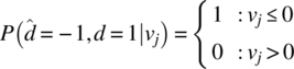
The Wagner code is a single‐error‐correcting block code denoted by (N, N − 1) where N is the block length containing N − 1 information bits. A typical block structure for the (N, N − 1) Wagner code is shown in Figure 8.28 where di = {0,1}, i = 1, 2, …, N − 1 represents the binary information bits and the single parity bit dN is determined from the modulo‐2 sum of the information bits as ![]() . The Wagner decoding process is quite simple. A hard decision is made to obtain an estimate of each received bit and the corresponding soft decisions are saved. A modulo‐2 addition is then performed on the five information bits and the parity bit. If the resulting parity bit is zero, the character is assumed to be correct. However, if the parity is one, the bit estimate corresponding to the smallest soft‐decision magnitude is inverted and the character is declared as being correct.
. The Wagner decoding process is quite simple. A hard decision is made to obtain an estimate of each received bit and the corresponding soft decisions are saved. A modulo‐2 addition is then performed on the five information bits and the parity bit. If the resulting parity bit is zero, the character is assumed to be correct. However, if the parity is one, the bit estimate corresponding to the smallest soft‐decision magnitude is inverted and the character is declared as being correct.

FIGURE 8.28 Wagner code structure.
The (6,5) Wagner code is sometimes applied to 7‐bit American Standard Code for Information Interchange (ASCII) character transmission. The first bit of the ASCII character is the start bit, which is followed by five information bits, and the seventh bit is the stop bit as shown in Figure 8.29. The start and stop bits are space or binary zero bits which are normally used for synchronization. In this situation, the Wagner coding is performed by replacing the stop bit with the parity bit formed as ![]() with
with ![]() , so the (6,5) Wagner code includes to the information bits and the stop bit. With this coding structure, the start bit is available for character synchronization.
, so the (6,5) Wagner code includes to the information bits and the stop bit. With this coding structure, the start bit is available for character synchronization.

FIGURE 8.29 Seven‐bit ASCII character with Wagner coding.
When differential coding is applied to the source data, as for example with compatible shift keying (CSK), the demodulation processing will result in two contiguous bit errors for every single‐error event. Therefore, to ensure detection of single‐error events, the parity check must be performed on every other bit. In this case, the start bit is used as the parity bit and is chosen to satisfy odd parity as ![]() with
with ![]() . Note that the parity check will detect all single‐error events with differential encoding; however, special consideration must be given to pairs of bit errors that span two adjacent characters because a detection error in the stop bit position will result in an error in the start (parity) bit in the next character. To ensure proper decoding in this case, a total of eight magnitude bits must be compared prior to the error correction. When the parity check fails on the current character block and the smallest magnitude is associated with the stop bit of the preceding character block, then the current parity bit is also assumed to be in error also and no error correction is performed on the current information bits.
. Note that the parity check will detect all single‐error events with differential encoding; however, special consideration must be given to pairs of bit errors that span two adjacent characters because a detection error in the stop bit position will result in an error in the start (parity) bit in the next character. To ensure proper decoding in this case, a total of eight magnitude bits must be compared prior to the error correction. When the parity check fails on the current character block and the smallest magnitude is associated with the stop bit of the preceding character block, then the current parity bit is also assumed to be in error also and no error correction is performed on the current information bits.
In the following sections, the character‐error performance of the Wagner code is examined. First, approximate expressions for the character‐error probability are developed for the three embodiments of the Wagner code discussed earlier, namely, the raw (N, N − 1) Wagner code, and Wagner coding applied to the 7‐bit ASCII character with and without differential encoding. The results of these analyses are approximate because the location of the bit in error is assumed to be known. The theoretical character‐error performance is then established based on using the soft decisions to identify the most likely bit to be in error. This analysis is exact in the sense that the soft decisions are used to locate the most probable bit in error.
8.10.1 Wagner Code Performance Approximation
The character‐error performance of a Wagner coded block can be approximated by assuming that all single errors are corrected and that all other error conditions are uncorrected and result in a character error. In this case, the character‐error probability of the raw (N, N − 1) Wagner code is simply
where the probability of a correct character, under the assumption of independent error events with probability Pbe, is given by
This result is based on the binomial distribution [53] and Pbe is the bit‐error probability of the underlying waveform modulation.
For the Wagner coded 7‐bit ASCII character without differential coding, the probability of a correct character is given by

With differential coding, the 7‐bit ASCII character is correctly decoded if a single bit‐error occurs among the six information bits. An error in the parity bit results in an error in the following information bits so the ASCII character cannot be corrected. The resulting probability of a correct character is then

The approximate performance results for the raw (N, N − 1) Wagner code are shown in Figure 8.30 for antipodal waveform modulation with AWGN. Figure 8.31 shows the approximate performance when the Wagner coded is applied to the 7‐bit ASCII character as discussed before. The signal‐to‐noise ratio (γc) for the underlying antipodal signaling of the coded bits is expressed in term to the code‐bit bandwidth 1/Tc, where Tc is the duration of the coded bit. The performance, however, is plotted as a function of the signal‐to‐noise ratio (γb) measured in the information bit bandwidth 1/Tb and the relationship is given by


FIGURE 8.30 Approximate performance of Wagner coded data (N‐bit character).
FIGURE 8.31 Approximate performance of Wagner coded data (7‐bit ASCII character).
For the raw Wagner code, ![]() and for the Wagner coded 7‐bit ASCII character Tb/Tc = 7/5 (= 1.46 dB).
and for the Wagner coded 7‐bit ASCII character Tb/Tc = 7/5 (= 1.46 dB).
8.10.2 (N, N − 1) Wagner Code Performance
In this section, the relationship between the bit‐error probability at the input to the Wagner decoder and the resulting character‐error probability at the decoder output is established. The theoretical performance in the AWGN channel is examined and the results are compared to Monte Carlo simulation results. The theoretical results apply for antipodal signaling such as BPSK, QPSK, OQPSK, or minimum shift keying (MSK); however, the simulation results are based on MSK waveform modulation with ideal symbol timing and phase tracking in the demodulator.
The general expression for the probability of a correctly received Wagner coded block is given by

When the noise is independent and identically distributed (iid) from bit to bit, this result can be expressed as

In the remainder of this section, the probability of correctly locating a single‐error event is analyzed using the stored soft decisions out of the optimally sampled matched filter.
The location of a single‐error event in the j‐th bit is based upon the magnitude zj of the j‐th decision variable vj being less than the magnitudes zi of all the other bit decision variables vi, i = 1, …, N such that i ≠ j. Given the transmitted bit sequence {di} and the received sequence {![]() }, the probability of correctly locating the error is given by the general expression
}, the probability of correctly locating the error is given by the general expression
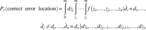
where f(−) is the conditional joint density function of the random variables ![]() . With independent source data, a memoryless channel, and ideal receiver timing, the AWGN channel decision variables, vi, are iid with distribution N(di, σn) for which the earlier result specializes to
. With independent source data, a memoryless channel, and ideal receiver timing, the AWGN channel decision variables, vi, are iid with distribution N(di, σn) for which the earlier result specializes to

The two conditioned distributions are found from a form of Bayes rule given by

Conditioning on an error event, that is, ![]() , the following relationships apply
, the following relationships apply

and
Upon combining these results with the normal distribution ![]() , the numerator in (8.58) becomes
, the numerator in (8.58) becomes

Using this result to evaluate the denominator in (8.58) conditioned on an error, it is noted that the denominator is simply the probability of a bit error, that is,

Since these results apply for vj > 0, upon substituting zj for vj in (8.61) the solution to (8.58) becomes
Evaluation of (8.58) conditioned on a correct decision, that is, ![]() , and proceeding in a similar manner leads to the conditional distribution
, and proceeding in a similar manner leads to the conditional distribution

Using (8.64) to evaluate the second integral in (8.57) results in

where Q(x) = 1 − Φ(x) and Φ(x) is the probability integral. Substituting (8.65) and (8.63) into (8.57) and, in turn, substituting (8.57) into the expression (8.55) for Pcc gives

This expression is computed numerically and the result is used to compute the character‐error probability expressed as
The solid curves in Figures 8.32 and 8.33 show the performance as a function of Eb/No for the (6,5) and (13,12) Wagner codes, respectively. The numerical integration is based on a resolution of 20 samples for each standard deviation σn over a range of 10 standard deviations above the mean value at zj = |dj|. The discrete circled data points for the (6,5) Wagner code are based on Monte Carlo simulations using 500 Kbits at each signal‐to‐noise ratio. Upon comparing these results with the approximations in Figure 8.30, it is seen that the approximate results are optimistic by about 1.0 dB at Pce = 10−5; owing to the fact that the bit‐error locations were assumed to be known.

FIGURE 8.32 Performance of MSK demodulator with (6,5) Wagner code.

FIGURE 8.33 Performance of MSK demodulator with (13,12) Wagner code.
The dotted curve in Figures 8.32 and 8.33 represent the character‐error performance if the information bits were not coded with the parity bit. These results are evaluated as
for N = 5 and 12, respectively, and they provide a reference for determining the coding gain of the Wagner coded characters which is about 2.0 dB at Pce = 10−5. The dotted curve in these figures is simply the uncoded bit‐error performance of antipodal signaling and is used to compute uncoded (5,5) and (12,12) Pce as a point of reference.
8.11 CONVOLUTIONAL CODES
The convolutional decoding discussed in this section focuses on the Viterbi decoding algorithm as it applies to a trellis decoding structure. Prior to the discovery of the trellis decoding structure, sequential decoding of convolutional codes, described by Wozencraft [54] and Fano [55], was used. Sequential decoding is based on metric computations on various branches through a code‐tree decoding structure [56]. In this case, the decoded data is associated with the branches or paths through the code tree that yield the largest metric. Heller and Jacobs [57] compare the advantages and disadvantages of the Viterbi and sequential decoding techniques in consideration of error performance, decoder delay, decoder termination sequences, code rates, quantization, and the sensitivity to channel conditions. The processing complexity is a major factor that distinguishes these two decoding procedures and, by this measure, Viterbi decoding is applicable to short constraint length codes (K ≤ 9); otherwise, the sequential decoding is more processing efficient.
The following description of convolutional coding draws upon the vast resource of research and publications on the subject [58–64] and other references cited throughout this section. Convolutional codes, unlike block codes, do not involve algebraic concepts in the decoding process and, therefore, result in more intuitive and, to some extent, straightforward processing algorithms. Throughout the following descriptions, binary data is considered and sequences are represented by polynomials ![]() with binary coefficients bi ∈ {1,0}. In this case, multiplication and summation of polynomials is performed using GF(2) arithmetic. For example, multiplication of two polynomials f(x) and f′(x) corresponds the coefficient multiplication
with binary coefficients bi ∈ {1,0}. In this case, multiplication and summation of polynomials is performed using GF(2) arithmetic. For example, multiplication of two polynomials f(x) and f′(x) corresponds the coefficient multiplication ![]() and summation is simply the modulo‐2 summation of the bi and
and summation is simply the modulo‐2 summation of the bi and ![]() coefficients.
coefficients.
Convolutional encoders accept a continuous stream of source data at the rate Rb bps and generate a continuous stream of code bits, at a rate of ![]() where rc is the code rate, defined as
where rc is the code rate, defined as
The parameter k represents the number of source data bits, corresponding to a q‐ary symbol (q = 2k), that are entered into the encoder each code block and n represents the corresponding number of coded bits.
A single parity bit is influenced by υ = kK source bits and the n encoder parity bits are generated by the convolutional sum, expressed as
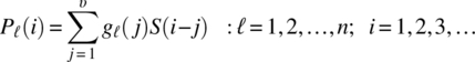
where gℓ(j) represents the ℓ‐th subgenerator of the code, S(j) is the stored array of source bits, and Pℓ(i) are the output parity bits corresponding to the ℓ‐th subgenerator. The parameter K is the constraint length of the code and corresponds to the number of stored M‐ary symbols during each code block. The index i, corresponding to the source data, can be arbitrarily long, distinguishing the convolutional codes from fixed‐length block codes. The encoder described by (8.70) can be viewed as a transversal, or finite impulse response (FIR), filter with unit‐pulse response described by the code generator.
The following description of the convolutional encoder is characterized in terms of the coding interval, or code block,18 defined as the encoder processing required to generate n parity bits in response to an input symbol of k source bits. This significantly simplifies the convolutional encoding and decoding description and notation. In the demodulator, the convolutional decoding is analogous to characterizing the trellis decoding as a recursion of multistate symbol decoding intervals.19 The encoding and decoding recognizes the correlative properties of preceding symbols, for example, the preceding K − 1 source symbols are processed in the encoder as described in the following.
In general, the convolutional encoder is implemented using binary arithmetic to compute the parity symbols by clocking a block of k source bits into shift registers and computing the corresponding n parity bits over the υ source bits stored in the encoder memory. To maintain real‐time operation, the duration of the n‐tuple of parity bits must equal the input symbol duration. The implementation of a GF(2k) convolution encoder is shown in Figure 8.34 where the binary arithmetic involves exclusive‐or operations.

FIGURE 8.34 Generalized GF(2k) nonsystematic convolutional encoder (rate rc = k/n, constraint length K).
The implementation in Figure 8.34 corresponds to one code block with the most recent k‐bit source symbol corresponding to the storage location 1 with the previous K − 1 symbols in the storage locations 2 through K. Following the message of length Tm seconds, the kK flush bits are used to return the encoder to the initial encoder state. Typically, the encoder is initialized to the zero state. The flush bits are also used in the decoder as described in Section 8.11.2. Each source symbol corresponds to a (k − 1)‐dimensional polynomial
where the bit bl0 is the rightmost or LSB of the input symbol. Taken collectively, the entire K symbols are denoted as the (υ − 1)‐dimensional polynomial
In Figure 8.34, the dotted lines, connecting the stored symbols to the subgenerators of the code, denote multiple connections from each subgenerator corresponding to the binary‐one coefficients of the (υ − 1)‐dimensional generator polynomial, expressed as
In the context of the code‐block processing, the subgenerators and stored data bits can be viewed as vectors with the parity formed by the scalar product ![]() .
.
An important consideration in the modulator encoding is the mapping of the code bits20 to the waveform modulation symbol as depicted in Figure 8.35 [65, 66]. The encoder shown in Figure 8.34 results in a nonsystematic code, in that the coded output contains only parity‐check bits; however, the code‐bit mapping also applies to systematic codes that include the k source bits plus n − k appended parity‐check bits. In either case, the information bits or the most significant bit (MSB) parity‐check bits must be mapped to the most protected states of the modulated waveform. If an interleaver is used, the number of interleaver columns is selected to accommodate an integer number of transmitted symbol. For example, for a rate rc = 1/n code using MPSK symbol modulation with modulation efficiency ![]() and n = multiples of rm, a row‐column interleaver may be designed with rm columns and n/rm rows. In this example, rate matching is not necessary; however, puncturing of low‐rate codes has many advantages and requires rate matching to the symbol modulation waveform.
and n = multiples of rm, a row‐column interleaver may be designed with rm columns and n/rm rows. In this example, rate matching is not necessary; however, puncturing of low‐rate codes has many advantages and requires rate matching to the symbol modulation waveform.

FIGURE 8.35 Mapping of code bits to modulation symbols.
Puncturing is a process in which certain parity‐check bits are not transmitted to realize a higher code rate than that of the underlying convolutional code. Although the resulting coding gain is reduced, the symbol bandwidth W is also reduced thus increasing the spectral efficiency, defined as, rs = Rb/W bits/s/Hz. Alternately, the symbol rate may remain the same thus increasing the data throughput time. In either event, puncturing provides for tailoring the message transmission to the channel conditions. When puncturing is used, it is only applied to the parity‐check bits, that is, the source bits of a systematic code are not punctured. Optimum puncturing of low‐rate convolutional codes is discussed in Section 8.11.7. Appendix 8A provides a list convolutional code puncturing patterns found by Yasuda et al. [67], for punctured code rates (n − 1)/n with n = 3 through 14 and constraint length ν = 2 through 8. The punctured codes are based on the underlying rate 1/2 codes with the same constraint lengths. The rate matching function in Figure 8.35 identifies and eliminates the punctured parity‐check bits and prioritizes and assigns the surviving bits in the interleaver.
Referring again to Figure 8.34, rate‐matching parity‐check bits are priority ordered and entered column by column into a row–column interleaver with the highest priority bits in the MSB (leftmost) columns. The information bits of a systematic code are always assigned the highest priority. The interleaver is emptied row by row and mapped to the symbol modulator with the highest priority row bits assigned to the MSB of the modulation states, thus providing the most protection. Gray coding prior to the modulation symbol mapping provides the most protection from demodulator symbol errors. For example, consider that three contiguous code blocks of the rate 1/3 convolutional encoder in Figure 8.34 are entered into a 3 × 3 block interleaver. The nine parity‐check bits, Pℓ, are assigned to the block interleaver, gray coded, and then mapped to the 8PSK modulator phase constellation as shown in Figure 8.36. The ordering of the bits (P9,P8,P7) corresponds to the three consecutive MSB bits of the encoder. For example, P9 corresponds to the parity‐check bit bm2, of the first code‐block modulator polynomial

FIGURE 8.36 Example of rate matching for (3,9) convolutional encoder (3 × 3 block interleaver, gray coding, and 8PSK modulation).
In terms of (8.70), P9 = P3(1), P8 = P3(2), and P7 = P3(3). The mapping of the code bits to the symbol modulation is discussed again in Section 8.12.2 in the context of concatenated convolutional codes where the code block is defined as the interleaver length that ranges from 128 to over 16,384 information bits. This is a significantly different requirement; in that, the number of transmitted code bits corresponding to the interleaver plus flushing bits must be integrally related to the number of transmitted symbols.
Gray coding is used to minimize the error events in a noisy channel and, upon examining the phase constellation, it is seen that the first‐ and second‐order modulator bits are the most protected bits. In this example, the entire interleaved parity set is transmitted in the code‐block interval using three consecutive phase modulated symbols. Increasing the number of interleaver columns and filling the interleaver across several code blocks provides for improved mitigation of channel fading at the expense of throughput delay.
Beginning with the commonly used binary convolutional encoder, the following sections examine specific convolutional encoder configurations and the associated decoding complexity and performance characteristics.
8.11.1 Binary Convolutional Coding and Trellis Decoding
The binary convolutional code is characterized by entering one source bit into the encoder memory array each code block. This corresponds to k = 1 in Figure 8.34 with the K encoder memory consisting of K bits. The widely used rate 1/2 convolutional code with constraint length K = 7 provides excellent coding gain with reasonable complexity; however, the following description of the rate 1/2, K = 3 binary convolutional encoder provides all of the essential encoding and decoding concepts necessary to implement the more involved coding structures.
The coding and decoding of the simple, and relatively easy to understand, rate 1/2, K = 3 encoder is shown in Figure 8.37. The structure follows directly for the general implementation shown in Figure 8.34 using k = 1, K = 3 and the two subgenerators g1(x) and g2(x).

FIGURE 8.37 Binary, rate 1/2, K = 3, nonsystematic convolutional encoder (g1(x) = x2 + x + 1, g2(x) = x2 + 1).
The K = 3 encoder stores K − 1 previous bits in locations 2 and 3 and with current bit of the input source data in location 1. The K − 1 bits represent the state of the encoder so, for this binary convolution encoder, there are 2K−1 = 4 states. The encoder memory is initialized to zero and the following example uses the input data sequence of 1011010010…. The first bit into the encoder is 1, the leftmost bit, and, in keeping the convolutional sum, the input data is time‐reversed yielding,21 …0100101101. Based on this description, the encoder output is developed as shown in Table 8.11. The code bits are then processed as shown in Figure 8.35 and the modulated symbols are transmitted through the channel to the receiver.
TABLE 8.11 Example of Binary Rate 1/2, K = 3 Convolutional Encoding
| Source Bit 1 | Encoder State Bits 2,3 | Parity Bits (1,2) | ||
| 1 | 0 | 0 | 1 | 1 |
| 0 | 1 | 0 | 1 | 1 |
| 1 | 0 | 1 | 0 | 0 |
| 1 | 1 | 0 | 0 | 1 |
| 0 | 1 | 1 | 0 | 1 |
| 1 | 0 | 1 | 0 | 0 |
| 0 | 1 | 0 | 1 | 0 |
| 0 | 0 | 1 | 1 | 1 |
| 1 | 0 | 0 | 1 | 1 |
| 0 | 1 | 0 | 1 | 0 |
| ⋯ | 0 | 1 | ⋯ | ⋯ |
8.11.2 Trellis Decoding of Binary Convolutional Codes
The maximum‐likelihood decoding of convolutional codes was published by Viterbi [68] in 1967. This paved the way for further research in what has become known as the Viterbi algorithm [69]. Forney [70, 71], rigorously showed that the Viterbi algorithm results in maximum‐likelihood decoding, and Heller [72, 73] is credited with the discovery of efficient decoding techniques using the Viterbi algorithm.
In the following, description of the trellis decoding of convolutional codes is based on the relatively straightforward binary, rate 1/2, K = 3 code, recognizing that more powerful convolutional codes use exactly the same, albeit more involved, decoding algorithms. The decoding starts by identifying the four‐state trellis decoder and the corresponding binary representations of the four states as indicated in Figure 8.38. The parameters of the generalized k‐ary trellis decoder in Figure 8.34 are identified in Table 8.12 with the numerical values corresponding to the example decoder in Figure 8.38. In general, the trellis diagram of a rate k/n convolutional code has 2k(K−1) states with 2k transitions emanating from each source state and terminating on each termination state.

FIGURE 8.38 Description of convolutional code Trellis decoder (binary, rate 1/2, K = 3).
TABLE 8.12 Generalized Convolution Decoder Parameters
| Parameter | Description | Example Value |
| k | Input source bits per encoding block | 1 |
| n | Output code bits (parity) | 2 |
| k/n | Code rate | 1/2 |
| K | Constraint length | 3 |
| K − 1 | Trellis buildup and flushing transitions | 2 |
| kK | Encoder bits and stuff bits | 2 |
| 2k(K−1) | Encoder and trellis decoder states | 4 |
| 2k | Trellis branches emanating from and terminating on each state | 2 |
| Ndep | Trellis depth (symbols) before removing data estimates (4 or 5 constraint lengths)a | 15 |
aFor high‐rate codes (3/4 and higher), trellis depths of 8 or 9 constraint lengths are required.
By way of explanation, the decoding states in Figure 8.38 are represented by the state vectors ![]() with elements αi,j: j = 0, …, 3 denoted as the state metric corresponding to each of the trellis states. It will be seen that the state metrics αi,j are updated with estimates of the received data at each state transition. The dark gray state transition lines are shown to indicate that these transitions are not required as the trellis is building up when starting at the known zero initial state of the encoder. For short messages or short decoding depths, the decoder Eb/No performance is improved somewhat by not including these transition; however, the decoder synchronization is more problematic, in that the first code‐bit word must be synchronized with the SOM preamble. On the other hand, for long messages, that can tolerate longer trellis depths, the inclusion of these transitions is not as important because, with a trellis depth in excess of four constraint lengths, the trellis processing essentially eliminates the incorrect paths through the maximum‐likelihood decisions at each state transition.22
with elements αi,j: j = 0, …, 3 denoted as the state metric corresponding to each of the trellis states. It will be seen that the state metrics αi,j are updated with estimates of the received data at each state transition. The dark gray state transition lines are shown to indicate that these transitions are not required as the trellis is building up when starting at the known zero initial state of the encoder. For short messages or short decoding depths, the decoder Eb/No performance is improved somewhat by not including these transition; however, the decoder synchronization is more problematic, in that the first code‐bit word must be synchronized with the SOM preamble. On the other hand, for long messages, that can tolerate longer trellis depths, the inclusion of these transitions is not as important because, with a trellis depth in excess of four constraint lengths, the trellis processing essentially eliminates the incorrect paths through the maximum‐likelihood decisions at each state transition.22
The self‐synchronizing characteristic of the trellis decoder allows for message decoding in random data without knowledge of the SOM. For example, after initializing the state metrics, α0,j, to zero, if the decoding is not correctly synchronized with the received code‐bit word, the surviving metrics at each state, after about four constraint lengths, will appear as random variables. In this event, the state metric accumulators are re‐initialized, the code‐bit word timing is shifted, and the processing is repeated until a dominant metric is observed indicating code synchronization.
The dark gray state transition lines indicate the transitions that are not associated with the trellis flushing required to drive the trellis to the known all‐zero state of the encoder following the message bits. The two (in general kK) zero flushing bits are appended to the message bits as indicate in Figure 8.38.
The details of the trellis decoding are described by the transition processing shown in Figure 8.39. The state transition is depicted from the source state to the termination state denoted by the state vectors ![]() and
and ![]() . As a practical matter, only the two state vectors
. As a practical matter, only the two state vectors ![]() and
and ![]() , their respective elements αs,j = αi−1,j and αt,j = αi,j, and the detected data estimate
, their respective elements αs,j = αi−1,j and αt,j = αi,j, and the detected data estimate ![]() are required for the entire trellis decoding. This simplicity results from the add–compare–select (ACS) function of the max(a,b) algorithm and, for a sufficiently long trellis depths, leads to maximum‐likelihood data decoding [68].
are required for the entire trellis decoding. This simplicity results from the add–compare–select (ACS) function of the max(a,b) algorithm and, for a sufficiently long trellis depths, leads to maximum‐likelihood data decoding [68].

FIGURE 8.39 Trellis decoding state transition processing (binary (k = 1), rate 1/2, K = 3,  ).
).
As indicated, the state transitions in Figure 8.39 are only shown for the source data estimate ![]() and the remaining processing for
and the remaining processing for ![]() is implicit. The source states j = 0, …, 3 are represented by the binary equivalents j = (b2,b1)b that are concatenated with the source data estimate
is implicit. The source states j = 0, …, 3 are represented by the binary equivalents j = (b2,b1)b that are concatenated with the source data estimate ![]() denoted23 as
denoted23 as ![]() . The rightmost bits of the concatenation correspond, or point, to the termination state, and by convention the transitions corresponding to
. The rightmost bits of the concatenation correspond, or point, to the termination state, and by convention the transitions corresponding to ![]() are denoted by the dashes state transition lines. When the
are denoted by the dashes state transition lines. When the ![]() source data estimate is included, two state transitions will emanate from each source state and terminate on the termination states as indicated in Table 8.12. As mentioned before, the two transitions that terminate on state j = 0 correspond to
source data estimate is included, two state transitions will emanate from each source state and terminate on the termination states as indicated in Table 8.12. As mentioned before, the two transitions that terminate on state j = 0 correspond to ![]() with the source states identified as (b2,b1) = (0,0) and (1,0) corresponding to j = 0 and 2. For each state transition, there is an associated source state metric αs,j, metric update Δαm, and termination state j′. Therefore, the termination state must select the maximum αs,j + Δαm of all source states terminating on j′. This is shown in Figure 8.39 as the ACS function corresponding to the termination states j′ = 0 and 2.
with the source states identified as (b2,b1) = (0,0) and (1,0) corresponding to j = 0 and 2. For each state transition, there is an associated source state metric αs,j, metric update Δαm, and termination state j′. Therefore, the termination state must select the maximum αs,j + Δαm of all source states terminating on j′. This is shown in Figure 8.39 as the ACS function corresponding to the termination states j′ = 0 and 2.
The parity bits (p2,p1) corresponding to each transition are determined from knowledge of the convolutional encoder and are determined in the same manner as in the encoder. Several important observations are that each state transition is characterized as having a Hamming distance24 of two, the parity bits associated with transitions terminating on the same state are antipodal, and the metric updates Δαm are associated with the parity bits with m = (p2,p1)b = 0, …, 3. The parity bits form the link to the received data; in that, the received parity bits at the demodulator matched filter output are correlated with each set of transition parity bits (p2,p1) with the correlation equal to the state transition update Δαm. The details in the computation of Δαm are discussed in the following.
The link between the trellis decoder and the convolutional encoder is found in the received symbols that contain noise corrupted estimates of the modulated waveform symbols. For example, consider the BPSK modulated waveform with phase modulation ![]() , where
, where ![]() 25 represents the two unipolar consecutive code bits corresponding to a code‐bit word; these bits are referred to as the parity bits
25 represents the two unipolar consecutive code bits corresponding to a code‐bit word; these bits are referred to as the parity bits ![]() in the earlier description of the trellis decoding. The corresponding demodulator matched filter samples are denoted as {ĉ2, ĉ1}, where
in the earlier description of the trellis decoding. The corresponding demodulator matched filter samples are denoted as {ĉ2, ĉ1}, where ![]() are the independent noisy estimates of
are the independent noisy estimates of ![]() . With ideal AGC and phase tracking, the receiver estimate, ĉℓ, is expressed as
. With ideal AGC and phase tracking, the receiver estimate, ĉℓ, is expressed as

where Es/No is the symbol energy‐to‐noise density ratio, held constant by the ideal gain control and nℓ is a zero‐mean, unit‐variance, independent Gaussian noise random variable.
The binary code bits corresponding to each state transition in Figure 8.38 are represented by their bipolar equivalents as shown in Table 8.13.
TABLE 8.13 Unipolar to Bipolar State Conversion ![]()
| Index m | Trellis State | |||
| Unipolar | Bipolar | |||
| b2 | b1 | d2 | d1 | |
| 0 | 0 | 0 | 1 | 1 |
| 1 | 0 | 1 | 1 | −1 |
| 2 | 1 | 0 | −1 | 1 |
| 3 | 1 | 1 | −1 | −1 |
The correlation of the received code block estimates ![]() with the 2n|n=2 = 4 possible code‐bit combinations of the trellis bipolar state code‐bits
with the 2n|n=2 = 4 possible code‐bit combinations of the trellis bipolar state code‐bits ![]() ;
; ![]() results in the correlations26
results in the correlations26

As the processing continues through the trellis, the surviving metric, determined from the ACS decisions, will eventually integrate to a uniquely large metric providing reliable data decisions. The trellis integration length or depth (Ndep) of four to five constraint lengths is usually sufficient for a reliable data decision. Figure 8.40 summarizes the state transition processing described in Figures 8.38 and 8.39 and includes the storage of the data estimate ![]() that is concatenation with the data vector
that is concatenation with the data vector ![]() . After a trellis depth of Ndep transitions, the oldest data is removed from the data vector and output as the maximum‐likelihood decoded estimate of the corresponding source data.
. After a trellis depth of Ndep transitions, the oldest data is removed from the data vector and output as the maximum‐likelihood decoded estimate of the corresponding source data.

FIGURE 8.40 Summary of convolutional code trellis decoding (binary (k = 1), rate 1/2, K = 3).
As mentioned before, associated with each surviving state metric is a stored sequence of data estimates and, after Ndep received bits are process, the oldest bits in the stored sequence are output as the maximum‐likelihood estimate of the transmitted bits. This is referred to at the path history storage and Rader [74] discusses efficient memory management and trace‐back to the transmitted data estimate. Through the ACS decisions, made at each trellis state, all of the incorrect paths leading to the estimate of the transmitted data, Ndep‐bits earlier, tend to be eliminated so, with high probability, any of the stored data vectors associated with the surviving metrics can be used to recover the estimate of the transmitted data. However, for shorter trellis depths or short constraint lengths codes with lower throughput delays, the optimum transmitted data estimate must be taken from the stored data array associated with the maximum metric of the trellis states, that is, max(αs,j) : j = 0, …, 3. Upon completion of transition processing, the termination metrics αt,j are assigned to the source metrics αs,j and the decoding continues with a minimum of trellis memory. To avoid metric accumulation overflow, the maximum metric must be examined periodically and each metric reduced by a constant value if overflow is imminent.
8.11.3 Selection of Good Convolutional Codes
In general, the code generators are selected to ensure that the codes result in the maximal free distance27 and do not result in catastrophic error propagation [75] following an error event. Exhaustive computer search algorithms are run to determine the best code generator for specific code configurations [76, 77]. The search algorithms examine details of the encoding structure including those involving catastrophic error propagation and equivalent codes. Equivalent codes have properties involving the reciprocal, shifting, and ordering of subgenerators. For example, reversing the order of the subgenerators results in an equivalent code. The following convolutional codes, referred to as good codes, are based on the maximal free distance, dfree, criterion when used with Viterbi decoding of convolutional codes.
A useful characteristic of convolutional codes is the insensitivity to signal phase reversals when used with differential data coding. Convolutional codes exhibiting this feature are referred to as transparent convolutional codes in which complements of code words are also code words. A convolutional code is transparent if each subgenerator has an odd number of binary coefficients [78]. By examining the variations in the surviving metrics through the trellis decoder, an estimate of the channel quality and the received signal‐to‐noise ratio are established. These estimates take advantage of the surviving state metric that increases at a constant rate in proportion to the received signal‐to‐noise ratio through the trellis decoder [78].
Good nonsystematic rate 1/n binary convolutional code generators for use with the Viterbi decoding algorithm were investigated by Odenwalder [76], and the results for rate 1/2 convolutional codes with constraint lengths 3 through 9 are listed in Table 8.14.28 Odenwalder’s results for rate 1/3 binary convolutional codes with constraint lengths 3 through 8 are listed in Table 8.15. Larsen [79] has extended Odenwalder’s results to include the respective constraint lengths 10 through 14 and 9 through 14, in these tables. The constraint length 9 codes listed in these tables are specified in the North American direct sequence CDMA (DS‐CDMA) Digital Cellular System Interim Standard (IS‐95) [80]. The rate 1/4 convolutional codes in Table 8.16 were found by Larson.29 The bit‐error performance dependence on Eb/No for the rate 1/2 code is examined in Section 8.11.8 for constraint lengths K = 4 through 9. Duet, Modestino, and Wismer [81] have extended the binary rate 1/n convolutional codes with maximum free distances to include code generators for n = 5, 6, 7, and 8; their results are listed in Tables 8.17, 8.18, 8.19, and 8.20 for constraint lengths 3 through 8.
TABLE 8.14 Rate 1/2 Nonsystematic Binary Convolutional Code Subgeneratorsa
| Constraint Length, K | Subgenerators (g1,g2) | dfree |
| 3 | 7,5 | 5 |
| 4 | 17,15 | 6 |
| 5 | 35,23 | 7 |
| 6 | 75,53 | 8 |
| 7 | 171,133 | 10 |
| 8 | 371,247 | 10 |
| 9 | 753,561b | 12 |
| 10 | 1545,1167 | 12 |
| 11 | 3661,2335 | 14 |
| 12 | 5723,4335 | 15 |
| 13 | 17661,10533 | 16 |
| 14 | 27123,21675 | 16 |
aLarsen [79]. Reproduced by permission of the IEEE.
bIS‐95 DS‐CDMA forward link speech encoder.
TABLE 8.15 Rate 1/3 Nonsystematic Binary Convolutional Code Subgeneratorsa
| Constraint Length, K | Subgenerators (g1,g2,g3) | dfree |
| 3 | 7,7,5 | 8 |
| 4 | 17,15,13 | 10 |
| 5 | 37,33,25 | 12 |
| 6 | 75,53,47 | 13 |
| 7 | 175,145,133b | 15 |
| 8 | 367,331,225 | 16 |
| 9 | 711,663,557c | 18 |
| 10 | 1633,1365,1117 | 20 |
| 11 | 3175,2671,2353 | 22 |
| 12 | 6265,5723,4767 | 24 |
| 13 | 17661,10675,10533 | 24 |
| 14 | 37133,35661,21645 | 26 |
aLarsen [79]. Reproduced by permission of the IEEE.
bThis code found by Larsen and Odenwalder. Odenwalder’s published code is (171,145,133) with dfree = 14
cIS‐95 DS‐CDMA reverse link speech encoder.
TABLE 8.16 Rate 1/4 Nonsystematic Binary Convolutional Code Subgeneratorsa
| Constraint Length, K | Subgenerators (g1,g2,g3,g4) | dfree |
| 3 | 7,7,7,5 | 10 |
| 4 | 17,15,15,13 | 13 |
| 5 | 37,33,27,25 | 16 |
| 6 | 75,71,67,53 | 18 |
| 7 | 163,147,135,135 | 20 |
| 8 | 357,313,275,235 | 22 |
| 9 | 745,733,535,463 | 24 |
| 10 | 1653,1633,1365,1117 | 27 |
| 11 | 3175,2671,2353,2387 | 29 |
| 12 | 7455,6265,5723,4767 | 32 |
| 13 | 16727,15573,12477,11145 | 33 |
| 14 | 35537,35527,23175,21113 | 36 |
aLarsen [79]. Reproduced by permission of the IEEE.
TABLE 8.17 Rate 1/5 Nonsystematic Binary Convolutional Code Subgeneratorsa
| Constraint Length, K | Subgenerators (g1,g2,g3,g4,g5) | dfree |
| 3 | 7,7,7,5,5 | 13 |
| 4 | 17,17,13,15,15 | 16 |
| 5 | 37,27,33,25,35 | 20 |
| 6 | 75,71,73,65,57 | 22 |
| 7 | 175,131,135,135,147 | 25 |
| 8 | 257,233,323,271,357 | 28 |
aDaut et al. [81]. Reproduced by permission of the IEEE.
TABLE 8.18 Rate 1/6 Nonsystematic Binary Convolutional Code Subgeneratorsa
| Constraint Length, K | Subgenerators (g1,g2,g3,g4,g5,g6) | dfree |
| 3 | 7,7,7,7,5,5 | 16 |
| 4 | 17,17,13,13,15,15 | 20 |
| 5 | 37,35,27,33,25,35 | 24 |
| 6 | 73,75,55,65,47,57 | 27 |
| 7 | 173,151,135,135,163,137 | 30 |
| 8 | 253,375,331,235,313,357 | 34 |
aDaut et al. [81]. Reproduced by permission of the IEEE.
TABLE 8.19 Rate 1/7 Nonsystematic Binary Convolutional Code Subgeneratorsa
| Constraint Length, K | Subgenerators (g1,g2,g3,g4,g5,g6,g7) | dfree |
| 3 | 7,7,7,7,5,5,5 | 18 |
| 4 | 17,17,13,13,13,15,15 | 23 |
| 5 | 35,27,25,27,33,35,37 | 28 |
| 6 | 53,75,65,75,47,67,57 | 32 |
| 7 | 165,145,173,135,135,147,137 | 36 |
| 8 | 275,253,375,331,235,313,357 | 40 |
aDaut et al. [81]. Reproduced by permission of the IEEE.
TABLE 8.20 Rate 1/8 Nonsystematic Binary Convolutional Code Subgeneratorsa
| Constraint Length, K | Subgenerators (g1,g2,g3,g4,g5,g6,g7,g8) | dfree |
| 3 | 7,7,5,5,5,7,7,7 | 21 |
| 4 | 17,17,13,13,13,15,15,17 | 26 |
| 5 | 37,33,25,25,35,33,27,37 | 32 |
| 6 | 57,73,51,65,75,47,67,57 | 36 |
| 7 | 153,111,165,173,135,135,147,137 | 40 |
| 8 | 275,275,253,371,331,235,313,357 | 45 |
aDaut et al. [81]. Reproduced by permission of the IEEE.
The code generators in Tables 8.14, 8.15, 8.16, 8.17, 8.18, 8.19, and 8.20 are based on the binary Hamming distance and, as such, represent good codes for binary signaling in which each of the coded bits is mapped into one symbol using, for example, BPSK or BFSK waveform modulation. Alternately, each pair of code bits generated by the rate 1/2 binary convolutional code can be mapped into a 4‐ary modulated symbol and consecutive groups of three code bits generated by a rate 1/3 binary convolutional code can be mapped to an 8‐ary modulated symbol. However, a nonbinary Hamming distance measure should be used when mapping the code bits to an M‐ary modulated symbol. In this regard, Trumpis [82] investigated good rate 1/2 and 1/3 binary convolutional codes based on nonbinary Hamming distances with corresponding 4‐ary and 8‐ary symbol mapping; the resulting code generators are listed in Tables 8.21 and 8.22.
TABLE 8.21 Rate 1/2 Nonsystematic Binary Convolutional Code Subgenerators for 4‐ary Signalinga
| Constraint Length, K | Subgenerators (g1,g2) |
| 3 | 7,5 |
| 4 | 15,12 |
| 5 | 32,25 |
| 6 | 75,57 |
| 7 | 133,176 |
aMichelson and Levesque [63]. Reproduced by permission of John Wiley & Sons, Inc.
TABLE 8.22 Rate 1/3 Nonsystematic Binary Convolutional Code Subgenerators for 8‐ary Signalinga
| Constraint Length, K | Subgenerators (g1,g2,g3) |
| 3 | 4,6,5 |
| 4 | 11,15,13 |
| 5 | 22,33,26 |
| 6 | 46,67,55 |
| 7 | 176,155,127 |
aMichelson and Levesque [63]. Reproduced by permission of John Wiley & Sons, Inc.
The preceding codes are all binary rate 1/n convolutional codes, and Paaske [77] has evaluated nonbinary rate (n − 1)/n convolutional codes and the subgenerators are listed in Tables 8.23 and 8.24 for the codes rates 2/3 and 3/4. Paaske’s work is based on Forney’s formulation [83, 84] of high‐rate convolutional codes where the parameter ν is defined as the constraint length. The topology of the rate (n − 1)/n encoder is similar to the general encoder shown in Figure 8.34. For these convolutional codes, the number of source‐bits input to the encoder memory each code block is k = n − 1. The example code, used to clarify the following description, is shown in Figure 8.41 and corresponds to the rate 3/4, constraint length 6, convolutional encoder listed in Table 8.24.
TABLE 8.23 Rate 2/3 Nonsystematic Nonbinary Convolutional Code Subgeneratorsa
| Constraint Length, ν | Subgenerators (g1,g2,g3) | dfree |
| 2 | 13,06,16 | 3 |
| 3 | 41,30,75 | 4 |
| 4 | 56,23,65 | 5 |
| 5 | 245,150,375 | 6 |
| 6 | 266,171,367 | 7 |
| 7 | 1225,0655,1574 | 8 |
| 9 | 4231,2550,7345 | 9 |
| 10 | 5516,2663,6451 | 10 |
aPaaske [77] by permission of the IEEE.
TABLE 8.24 Rate 3/4 Nonsystematic Nonbinary Convolutional Code Subgeneratorsa
| Constraint Length, ν | Subgenerators (g1,g2,g3,g4) | dfree |
| 3 | 400,630,521,701 | 4 |
| 5 | 442,270,141,763 | 5 |
| 6 | 472,215,113,764 | 6 |
| 8 | 4463,2470,1511,7022 | 7 |
| 9 | 4113,2246,1744,7721 | 8 |
aPaaske [77] by permission of the IEEE.

FIGURE 8.41 Rate 3/4, constraint length v = 6, K = 3, convolutional encoder.
In terms of the code‐block parity generator matrix G, Paaske defines as set of (n − 1 by n) generator matrices Gi: i = 0, …, K − 1 expressed as
where ![]() are n − 1‐dimensional column vectors with binary elements {1,0}. The subgenerators gℓ(x), defined by (8.73) and shown in Figure 8.34, are evaluated, in terms of the transpose of the k = n − 1 column vectors
are n − 1‐dimensional column vectors with binary elements {1,0}. The subgenerators gℓ(x), defined by (8.73) and shown in Figure 8.34, are evaluated, in terms of the transpose of the k = n − 1 column vectors ![]() , as
, as
In words, gℓ(x) is the sum of the transpose of the ℓ‐th column vector in Gi with the significance of the bits in descending order from right to left. For example, Paaske’s generator matrices for the rate 3/4, constraint length v = 6, convolutional code, shown in Figure 8.41, are listed in Table 8.25; the corresponding subgenerators gℓ(x) are listed in Table 8.26 using binary and octal notation.
TABLE 8.25 Paaske’s Generator Matrices for the Rate 3/4, Constraint Length 6, Convolutional Code
| G 0 | G 1 | G 2 | |||||||||
| 1 | 0 | 0 | 1 | 1 | 0 | 0 | 1 | 0 | 1 | 0 | 1 |
| 0 | 1 | 0 | 1 | 1 | 0 | 0 | 1 | 1 | 0 | 1 | 0 |
| 0 | 0 | 1 | 1 | 1 | 1 | 1 | 0 | 0 | 1 | 1 | 0 |
TABLE 8.26 Subgenerators for the Rate 3/4, Constraint Length 6, Convolutional Code
| Subgenerators | Binary | Octal |
| g1(x) | 100111010 | 472 |
| g2(x) | 010001101 | 215 |
| g3(x) | 001001011 | 113 |
| g4(x) | 111110100 | 764 |
Referring to the state transitions in the trellis diagram as emanating from a source state and converging on a termination state, the code bits associated with each of the transitions to a given termination state are important; in that, they influence the selection of the survivor at the termination states and ultimately the trellis decoding performance. For the rate 1/2, K = 3 binary trellis decoder, shown in Figure 8.38, there are only two transitions converging on each termination state and the corresponding Hamming distances between any two code words is: hd = {0,1,2}. However, with the unipolar‐to‐bipolar mapping di = 1 − 2bi, such that bi = {0,1} and di = {1,−1}, the, noise‐free, correlation response between any two code words is, from (8.76), ![]() . The maximum cross‐correlation,
. The maximum cross‐correlation, ![]() , corresponds to the received code‐word matching the transition code word leading to a correct survivor decision in the noise‐free case. Therefore, the matched filter or correlation detector responses dissimilar to the receive code word are either orthogonal or antipodal.
, corresponds to the received code‐word matching the transition code word leading to a correct survivor decision in the noise‐free case. Therefore, the matched filter or correlation detector responses dissimilar to the receive code word are either orthogonal or antipodal.
For a trellis decoder with a large number of trellis states with multiple source states converging on each termination state, it is processing efficient to store pointers to each source state and the corresponding transition code words. Using the rate 3/4, constraint length 6, K = 3 convolutional code in Figure 8.41 as an example, the 2k=3 = 8 source states (Si), converging on the selected termination state (Si+1), are depicted in Figure 8.42. The selected termination state identifies the binary source data in the k = 3‐bit encoder memory B−1,n and B and the eight different source states is determined by indexing the 3‐bit encoder memory B−2,m from 0 to 7. For each source state, the unique 4‐bit code word (CWm) is determine by applying the subgenerators gℓ(x) as expressed in (8.73) and identified in Table 8.24.

FIGURE 8.42 Convolutional code trellis decoding (8‐ary, rate 3/4, K = 3).
It is relatively easy to write a computer program to evaluate the encoder binary memory that identifies the source states, the input source data B, and the corresponding transition code words given the termination state as described earlier. In this evaluation, it is useful to write a procedure to convert from binary to integer and vice versa using the convention that the LSB is on the right. Computer simulations indicate that, for all 26 = 64 possible states, hd = {0,1,4} and the noise‐free cross‐correlation response between the received and transition code‐words is ![]() . Using the binomial coefficient, the number of combinations of the eight code words taken two at a time is
. Using the binomial coefficient, the number of combinations of the eight code words taken two at a time is ![]() and of these 28 combinations, 4 have cross‐correlations of +4 and 24 have cross‐correlations of zero.
and of these 28 combinations, 4 have cross‐correlations of +4 and 24 have cross‐correlations of zero.
8.11.4 Dual‐k Nonbinary Convolutional Codes
The dual‐k code is a nonbinary class of convolutional codes that are designed to be used with M‐ary symbol modulation. The dual‐k encoder shifts k input bits through dual (two) k‐bit registers and outputs dual (two) k‐bit symbols. Proakis [85] expresses the subgenerators gi(x) : i = 1, …, 2k for the dual‐k codes as follows:


Here, Ik is the k × k identity matrix. The dual‐3 code provides robust communications in a Rayleigh fading stressed environment using 8‐ary FSK symbol modulation and noncoherent detection [86, 87]. The dual‐3, ‐4, and ‐5 encoder subgenerators are tabulated in Table 8.27 and the dual‐3 encoder is shown in Figure 8.43.
TABLE 8.27 Dual‐3, ‐4, and ‐5 Convolutional Code Subgenerators
| Code | Subgeneratorsa | |
| Dual‐3 | g1, g2, g3 | (4,4), (2,2), (1,1) |
| g4, g5, g6 | (6,4), (1,2), (4,1) | |
| Dual‐4 | g1, g2, g3, g4 | (10,10), (4,4), (2,2), (1,1) |
| g5, g6, g7, g8 | (14,10), (2,4), (1,2), (10,1) | |
| Dual‐5 | g1, g2, g3, g4, g5 | (20,20), (10,10), (4,4), (2,2), (1,1) |
| g6, g7, g8, g9, g10 | (30,20), (4,10), (2,4), (1,2), (20,1) | |
aGroups of k‐bits are in octal notation with the LSB on the right.
FIGURE 8.43 Dual‐3 convolutional encoder.
8.11.5 Convolutional Code Transfer Function and Upper Bound on Performance
An important technique in the performance analysis of a convolutional code is the transfer function described by Odenwalder [76] and in a tutorial paper by Viterbi [88]. The convolutional code transfer function is derived from a state diagram [89] that highlights the Hamming distance properties of the code for various states through the trellis decoder. The transfer function properties are characterized as the ratio of the output to input states over a prescribed code sequence; however, since the convolution code is linear, the Hamming distance is independent of the selected output to input states so the all‐zero sequence is chosen because of its relative simplicity in interpreting the transfer function of the code.
The convolutional code transfer function is described using, as an example, the binary rate 1/2, constraint length K = 3 code shown in Figure 8.37 and the corresponding trellis diagram shown in Figure 8.38. The state diagram for this code is shown in Figure 8.44 and is based on an all‐zero data sequence with the data error branches converging on successive states and reemerging with the correct zero state at different points through the trellis. The distance between the correct code word 00 and the code word corresponding to the transition path is labeled Dd where d denotes the Hamming distance, so the distance from the state 00 to 01 labeled D2. In a like manner, the number of bit errors and the path length corresponding to the transition path are labeled N and L, respectively. These labels are easily determined from the trellis diagram of the code, as shown for this example code in Figure 8.38 where, for the assumed zero source data, a single bit error is indicated by the solid transition lines. In the state diagram description, the path length L is included with each transition path; however, when expressed in terms of the code transfer function, L will take on an integer exponent indicating the path length for a divergent path reemerging with the all‐zero path.

FIGURE 8.44 State diagram for binary, rate 1/2, K = 3, convolutional code.
The state diagram is used to compute the convolutional code transfer function by following the few simple rules shown in Figure 8.45.

FIGURE 8.45 State diagram reduction rules.
Defining the transfer function as T(N,L,D) = y0/x0 and applying the appropriate rules in Figure 8.45 results in the expression

Referring to the last equality in (8.81), the exponents of the parameters N, L, and D indicate, respectively, the number of decoded bit errors that occurred before reemerging with the all‐zero path, the number of path lengths prior to reemerging with the all‐zero path, and the Hamming distance of the code words over the path before reemerging with the all‐zero path. Therefore, the minimum distance for this example convolutional code is dmin = 5 and occurred over one path of 3 trellis transitions resulting in one bit error. The next smallest Hamming distance of 6 and occurred over two path lengths of 4 and 5 resulting in two bit errors per path for a total 4 bit‐errors, and so on. The number of bit errors corresponding to each Hamming distance is determined by differentiating (8.81) with respect to N and then setting N and L equal to one; the result is expressed as

For ideal BPSK waveform modulation and the AWGN channel, the probability of error for each incorrect path prior to reemerging with the all zero path is given by
where rc is the code rate, γb is the energy‐to‐noise‐density ratio measured in the data rate bandwidth, hd and np are the Hamming distance and number of bit errors for all paths associated with the Hamming distance. The overall bit‐error probability can be upper bounded by applying the union bound and, for the binary, rate rc = 1/2, K = 3 example code being considered, the bit‐error probability is upper bounded by

As stated previously, the decoding path length is important with short messages, and (8.84) and the last equality in (8.81) provide some insight on the impact of the trellis decoding length on the decoder performance. However, for long messages the trellis depth of four or five constraint lengths is not a performance limiting issue, aside from the message throughput delay.
Odenwalder [76] provides a convenient closed‐form solution for the upper bound on the bit‐error probability by using the inequality
Using this result, (8.84) is expressed as

The derivative of the convolutional code transfer functions for the binary rate 1/2 and 1/3 convolutional codes, listed in Tables 8.14 and 8.15, are shown in Tables 8.28 and 8.29 where
TABLE 8.28 Derivative of the Transfer Function of the Binary Rate 1/2 Convolutional Codea
| Constraint Length, K | |
| 3 | D5 + 4D6 + 12D7 + 32D8 + 80D9 + 192D10 + 448D11 + 1024D12 + 2304D13 + 5120D14 + ⋯ |
| 4 | 2D6 + 7D7 + 18D8 + 49D9 + 130D10 + 333D11 + 836D12 + 2069D13 + 5060D14 + 12255D15 + ⋯ |
| 5 | 4D7 + 12D8 + 20D9 + 72D10 + 225D11 + 500D12 + 1324D13 + 3680D14 + 8967D15 + 22270D16 + ⋯ |
| 6 | 2D8 + 36D9 + 32D10 + 62D11 + 332D12 + 701D13 + 2342D14 + 5503D15 + 12506D16 + 36234D17 + ⋯ |
| 7 | 36D10 + 211D12 + 1404D14 + 11633D16 + 77433D18 + 502690D20+ ⋯ |
aMichelson and Levesque [63]. Reproduced by permission of John Wiley & Sons.
TABLE 8.29 Derivative of the Transfer Function of the Binary Rate 1/3 Convolutional Codea
| Constraint Length, K | |
| 3 | 3D8 + 15D10 + 58D12 + 201D14 + 655D16 + 2052D18+ ⋯ |
| 4 | 6D10 + 6D12 + 58D14 + 118D16 + 507D18 + 1284D20 + 4323D22+ ⋯ |
| 5 | 12D12 + 12D14 + 56D16 + 320D18 + 693D20 + 2324D22 + 8380D24+ ⋯ |
| 6 | D13 + 8D14 + 26D15 + 20D16 + 19D17 + 62D18 + 86D19 + 204D20 + 420D21 + 710D22 + 1345D23 + ⋯ |
| 7 | 7D15 + 8D16 + 22D17 + 44D18 + 22D19 + 94D20 + 219D21 + 282D22 + 531D23 + 1104D24 + 1939D25 + ⋯ |
aMichelson and Levesque [63]. Reproduced by permission of John Wiley & Sons.
Similarly, the derivative of the convolutional code transfer functions for the rate 1/2 and 1/3 convolutional codes with 4‐ary and 8‐ary symbol modulations are listed in Tables 8.30 and 8.31. The subgenerators for these codes correspond to those listed in Tables 8.21 and 8.22 for 4‐ary and 8‐ary symbol modulations, respectively. The performance of these codes can be compared, without the need for detailed computer simulations, using (8.84), (8.85), and (8.87) with the appropriate polynomials in D given in the following tables.
TABLE 8.30 Derivative of the Transfer Function of the Binary Rate 1/2 Convolutional Code for 4‐ary Symbol Modulationa
| Constraint Length, K | |
| 3 | D3 + 4D4 + 12D5 + 32D6 + 80D7 + 192D8 + 448D9 + 1024D10 + 2304D11 + 5120D12 + ⋯ |
| 4 | D4 + 14D5 + 21D6 + 94D7 + 261D8 + 818D9 + 2173D10 + 6335D11 + 17220D12 +47518D13 + ⋯ |
| 5 | 3D5 + 15D6 + 22D7 + 196D8 + 398D9 + 1737D10 + 4728D11 + 15832D12 + 47491D13 +144170D14 + ⋯ |
| 6 | 9D6 + 14D7 + 62D8 + 212D9 + 874D10 + 2612D11 + 9032D12 + 28234D13 + 93511D14 +288974D15 + ⋯ |
| 7 | 7D7 + 39D8 + 104D9 + 352D10 + 1348D11 + 4540D12 + 14862D13 + 48120D14 +156480D15 + 505016D16 + ⋯ |
aMichelson and Levesque [63]. Reproduced by permission of John Wiley & Sons.
TABLE 8.31 Derivative of the Transfer Function of the Binary Rate 1/2 Convolutional Code for 8‐ary Symbol Modulationa
| Constraint Length, K | |
| 3 | D3 + 2D4 + 5D5 + 10D6 + 20D7 + 38D8 + 71D9 + 130D10 + 235D11 + 420D12 + ⋯ |
| 4 | D4 + 2D5 + 7D6 + 16D7 + 41D8 + 94D9 + 219D10 + 492D11 + 1101D12 + 2426D13 + ⋯ |
| 5 | D5 + 5D6 + 8D7 + 25D8 + 64D9 + 170D10 + 392D11 + 958D12 + 2270D13 + 5406D14 + ⋯ |
| 6 | D6 + 5D7 + 7D8 + 34D9 + 76D10 + 200D11 + 557D12 + 1280D13 + 3399D14 + 8202D15 + ⋯ |
| 7 | D7 + 4D8 + 8D9 + 49D10 + 92D11 + 186D12 + 764D13 + 1507D14 + 4198D15 + 10744D16 + ⋯ |
aMichelson and Levesque [63]. Reproduced by permission of John Wiley & Sons.
8.11.6 The Dual‐k Convolutional Code Transfer Function
The transfer function of a rate rc = 1/n dual‐k convolutional code, with ℓ transmissions of the code, is expressed as [64, 90],

Upon differentiating (8.88) with respect to N and evaluating the result for N, L = 1 results in the expression

Equation (8.89) is evaluated for n = 2, corresponding to the code rate rc = 1/2, and the resulting polynomial expressions in terms of D are summarized in Table 8.32 for ℓ = 1 through 4 with

TABLE 8.32 Derivative of the Transfer Function of the Nonbinary Dual‐3 Codea
| ℓ | |
| 1 | D4F(D) |
| 2 | D8F(D2) |
| 3 | D12F(D3) |
| 4 | D16F(D4) |
aWith F(D) = C0 + C1D + C2D2 + ⋯, the notation F(Dm) = C0 + C1Dm + C2D2m + ⋯.
In this case, the exponent of D is the Hamming distance of the q‐ary symbol with q = 8 corresponding to the transmissions of two 8‐ary FSK symbols‐per‐code. The underlying code, corresponding to ℓ = 1, has a minimum free distance of dfree = 4.
8.11.7 Code Puncturing and Concatenation
Code puncturing is a technique that involves deleting specified parity bits from an underlying convolutional code, with rate rc, to provide codes rates greater than rc, with a commensurate decrease in the coding gain. The puncturing is accomplished by the rate and symbol mapping functions shown in Figure 8.35 and, if the puncturing is performed judiciously, the decoding can be accomplished with very little change in decoding complexity. Cain et al. [91] identify subgenerators for the best codes, derived by periodically puncturing an underlying rate 1/2 convolutional code, to obtain code rates 2/3 and 3/4 with constraint lengths30 v = 2, …, 8. Yasuda et al. [67], identify subgenerators (see Appendix 8A) derived from the underlying rate 1/2 convolutional code, to obtain punctured codes rates (n − 1)/n for n = 3 through 14 with constraint length v = 2, …, 8. High‐rate codes that are generated in this manner and decoded using a trellis decoder are referred to as pragmatic trellis codes. Wolf and Zehavi [92] discuss punctured convolutional codes used to generate high‐rate codes in the generation of pragmatic punctured [93] (P2) trellis codes [94], for PSK and quadrature amplitude modulation (QAM) waveforms.
When the punctured codes are derived from an underlying lower rate code, the trellis decoding is essentially the same as that of the underlying code; however, there is an increase in complexity associated with synchronization and tracking of the puncturing location in the decoding trellis. The ability to select the code rate by simply selecting the puncturing configuration has many advantages. For example, by altering the puncturing configuration, a single convolutional decoding chip [95] can be configured to accommodate more efficient modulation waveforms or to adjust the code rate to maintain the message reliability under varying channel conditions.
Code concatenation is a technique in which two codes are operated in a serial configuration to increase the overall coding gain relative to that of a single code. This configuration consists of an outer and inner code that may be identical codes; however, a common configuration is to use an RS outer code with a convolutional inner code. Typically, the codes are separated by an interleaver to ensure that error bursts are randomly distributed between the codes. Forney [96] has proposed the concatenation of a 2K‐ary RS outer code with a constraint length K convolutional inner code separated by an L‐by‐M row‐column block interleaver. The RS symbol contains K bits and the block interleaver is filled row by row with L RS symbols and emptied column by column with M = 2K − 1 symbols. Odenwalder [97] examines the performance this concatenated code configuration. Proakis and Rahman [87] examine the performance of concatenated dual‐k codes.
Other applications of code concatenation involve the design of turbo and turbo‐like codes. These configurations may involve two or more convolutional codes with each code separated by block interleavers that are instrumental in the overall decoding performance. Concatenated convolutional coding is discussed in more detail in Section 8.12 with references to original research and additional reading.
8.11.8 Convolutional Code Performance Using the Viterbi Algorithm
The performance results using the Viterbi algorithm are shown in Figure 8.46 for rate 1/2 binary convolutional coding with constraint lengths of 4 through 9. The decoding trellis depth is four constraint lengths. The results are shown using hard limiting and virtually infinite quantization of the matched filtered symbol samples. The hard‐limiting performance is equivalent to 1‐bit quantization. For comparison, the ideal or theoretical performance of antipodal signaling with AWGN is shown as the dashed curve. The Monte Carlo simulation results are based on 5M bits for each signal‐to‐noise ratio less than 4 dB. To preserve the simulated performance measurement accuracies for larger signal‐to‐noise ratios, the number is increased 10 fold. Under these conditions, the 90% confidence limit for bit‐error probabilities on the order of 5 × 10⁻⁷ is ±1.6 × 10⁻⁷ or within ±32%. For the hard‐limited performance evaluation, the 4.5M bit Monte Carlo simulation is increased 10 fold for signal‐to‐noise ratios ≥6 dB.

FIGURE 8.46 Rate 1/2, convolutional decoding performance with constraint length and infinite and hard limiting quantization (trellis depth = 5K bits).
An important consideration, regarding the demodulator processing, is the quantization of the matched filter output sample that directly impacts the performance of the convolutional decoder [72]. For example, with the received signal level held constant by the AGC, the two‐level hard‐limiting simulation performance in Figure 8.46, results in about 2.1 dB loss in Eb/No performance at Pbe = 10−5 compared to the infinitely quantized performance. By contrast, the simulation performance results shown in Figure 8.47 indicates that the performance loss with 4‐ and 8‐level (2‐ and 3‐bit) quantization results in a, respective, performance loss of less than 0.2 and 0.1 dB compared to the performance with essentially infinite quantization.

FIGURE 8.47 Rate 1/2, K = 7, convolutional decoding performance with input quantization (trellis length = 30 bits).
The results indicate that the improvement in signal‐to‐noise ratio at Pbe = 10−7, relative to the uncoded performance, is about 4.2 dB for K = 4 with 8‐level quantization and about 2.0 dB with hard limiting. By way of contrast, with Pbe = 10−7 and K = 9, the performance with infinite quantization and hard limiting is 7.3 and 4.4 dB respectively. Furthermore, for large signal‐to‐noise ratios, there is about 0.5 dB of improvement in the signal‐to‐noise ratio with each unit increase in the constraint length.
Figure 8.48 shows the sensitivity of the performance to receiver AGC gain variations. The 3‐bit quantizer includes a sign bit and two magnitude bits with saturation occurring at 1.0 V so the magnitude bits are assigned as b12−1 + b02−2. It is important to note that under‐flow rounding is used in all of the simulation results. In the simulation program, the nominal baseband signal voltage at the quantizer input of is set to 0.707 V or 3 dB below the 1.0 V saturation level.

FIGURE 8.48 Rate 1/2, K = 7, convolutional decoding sensitivity to demodulator gain changes (input quantization = 3‐bits).
The results of the simulated performance show that the loss in Eb/No performance is within ±0.2 dB over a receiver gain variation of about ±12 dB. Furthermore, the results indicate that symmetrical performance with respect to the receiver gain variation is obtained by setting the nominal baseband signal to 0.707 V below the quantizer saturation; this is not a surprising result since the nominal receiver level was adjusted based on this analysis.
8.11.9 Performance of the Dual‐3 Convolutional Code Using 8‐ary FSK Modulation
The dual‐3 convolutional coded 8‐ary noncoherent FSK performance with AWGN is evaluated using the uncoded bit‐error probability expressed in (7.21) as

where ![]() . Equation (8.91) is labeled as the uncoded curve in Figure 8.49 and is used as the underlying bit‐error probability in the evaluation of the dual‐3 convolutional coded performance with AWGN. The signal‐to‐noise ratio γ is measured in the symbol rate bandwidth and is related to the bandwidth of the bit rate as γ = kγb. The performance of the dual‐3 coded noncoherent 8‐ary FSK waveform is evaluated using (8.89) with n = 2, corresponding to the code rate rc = 1/2, and diversity values of ℓ = 1 through 4.31 In the evaluation of (8.89), the terms Dx are replaced by Pbe(xγ) and the results are shown as the dashed curves in Figure 8.49 for the indicated diversities; these curves represent upper bounds on the performance as indicate by the first inequality in (8.86).
. Equation (8.91) is labeled as the uncoded curve in Figure 8.49 and is used as the underlying bit‐error probability in the evaluation of the dual‐3 convolutional coded performance with AWGN. The signal‐to‐noise ratio γ is measured in the symbol rate bandwidth and is related to the bandwidth of the bit rate as γ = kγb. The performance of the dual‐3 coded noncoherent 8‐ary FSK waveform is evaluated using (8.89) with n = 2, corresponding to the code rate rc = 1/2, and diversity values of ℓ = 1 through 4.31 In the evaluation of (8.89), the terms Dx are replaced by Pbe(xγ) and the results are shown as the dashed curves in Figure 8.49 for the indicated diversities; these curves represent upper bounds on the performance as indicate by the first inequality in (8.86).

FIGURE 8.49 Dual‐3 coded 8‐ary noncoherent FSK performance with AWGN.
The dashed curves in Figure 8.50 show the performance of the dual‐3 coded noncoherent 8‐ary FSK in a Rayleigh fading channel for the indicated diversities; the solid curve represents the uncoded performance with Rayleigh fading. The theoretical expressions for these results are based on the work of Odenwalder [98]. In this case, the bit‐error probability is evaluated by summing the coefficients (Ci) of the polynomial

where n = 2 corresponds to the rate 1/2 dual‐3 encoder. The coefficients Ci are those of F(D) expressed in (8.90) and the bit‐error probability is expressed as

where the factor involving k = 3 is used to convert from symbol errors to bit errors. Typically, only a few coefficient terms are required to obtain a good bound on Pbe and four are used to obtain the results in Figure 8.50. In (8.93), the probability Pi is the probability of an error in comparing two sequences that differ in i symbols and is evaluated as

where p is given by [99]


FIGURE 8.50 Dual‐3 coded 8‐ary noncoherent FSK performance with slow Rayleigh fading.
An easier evaluation of Pi, which applies for i ≥ 6, is [64, 90]

Equation (8.95) is plotted as the solid curve in Figure 8.50 and, using (8.94), (8.95), and (8.96), Equation (8.93) is plotted as the dashed curves. The notation <s> denotes the average value of s corresponding to the fading channel. The performance of the dual‐3 convolutional code in combating Raleigh fading is impressive and, referring to the performance with diversity applied to uncoded 8‐ary FSK in Section 20.9.5, the dual‐3 code without diversity, that is, with ℓ = 1, requires about 3 dB less Eb/No than the uncoded 8‐ary FSK modulation with ℓ = 4.
8.12 TURBO AND TURBO‐LIKE CODES
The discovery by Berrou, Glavieux, and Thitimajshima [1] of near‐optimum error correction coding and decoding, referred to as TCs, represents a major step toward achieving Shannon’s error‐free performance limit of Eb/No = −1.56 dB. Their revolutionary results describe an implementation involving the parallel concatenation of two convolutional codes, with an intervening random interleaver, that are decoded with multiple forward and backward iterations through a trellis decoder resulting in performance remarkably close to Shannon’s limit. This discovery sparked a new focus among analysts and practitioners that resulted in a unified theory32 of multiple PCCCs [100] with iterative decoding that performed within a few tenths of a decibel of Shannon’s limit. Divsalar and Pollara [101], Benedetto and Montorsi, and other researchers have substantiated the near Shannon‐limit performance of the PCCC and present generalized descriptions of an encoder/decoder suitable for personal communications service (PCS) and many other applications. This research has also led to a variety of alternative concatenated codes and a unified approach to their implementation [102]. For example, Benedetto, Montorsi, Divsalar, and Pollara have made major contributions to the understanding of the fundamentals of turbo coding and have extended the notion of iterative decoding to SCCCs [103]. Furthermore, their efforts have resulted in the description of a universal soft‐in soft‐out (SISO) decoding module [104] that is suitable for implementation using a variety of technologies: digital signal processors (DSPs), field programmable gate arrays (FPGAs), and application‐specific integrated circuits (ASICs). Divsalar [105] provides detailed descriptions of the coding and decoding of turbo and turbo‐like codes.
Compared to high‐constraint‐length convolutional codes, required to achieve moderately high coding gains, turbo‐like codes involve relatively short‐constraint‐length concatenated convolutional codes.33 An important distinction is that convolutional codes traditionally use nonrecursive convolutional (NRC) codes requiring, for example, constraint length K = 9 bits or 256 states, to achieve modest coding gains at relatively high signal‐to‐noise ratios. For example, a 256‐state convolutional code with a Viterbi decoder achieves ![]() dB at Pbe = 10−5 and the RSV concatenated code achieves
dB at Pbe = 10−5 and the RSV concatenated code achieves ![]() dB. On the other hand, TCs or PCCCs use recursive systematic convolutional (RSC) constituent codes (CCs) with 8 or 16 states and achieve
dB. On the other hand, TCs or PCCCs use recursive systematic convolutional (RSC) constituent codes (CCs) with 8 or 16 states and achieve ![]() dB at Pbe = 10−5. The SCCCs use two‐ or four‐state NRC and RSC CCs to achieve comparable performance. The selection of the code rates, interleaver lengths, and the number of demodulator decoder iterations is a major factor that influences the resulting performance. There is also an accompanying increase in decoder processing complexity that is inversely proportional to the code rate and proportional to the interleaver length and the number of iterations.
dB at Pbe = 10−5. The SCCCs use two‐ or four‐state NRC and RSC CCs to achieve comparable performance. The selection of the code rates, interleaver lengths, and the number of demodulator decoder iterations is a major factor that influences the resulting performance. There is also an accompanying increase in decoder processing complexity that is inversely proportional to the code rate and proportional to the interleaver length and the number of iterations.
The use of RSC codes is critical in that they result in infinite impulse response (IIR) convolutional codes that yield the largest effective free distance [106] for the turbo encoder. This large effective free distance provides the coding gain necessary to overcome the operation in extremely low signal‐to‐noise conditions when approaching the Shannon limit of Eb/No = −1.59 dB. Divsalar and McEliece use the notation (r, k, m) for the convolutional CC generators defined as the k × r matrix G(D) expressed as

where Q(D) is a primitive polynomial of degree m and Pi(D) of m‐degree polynomials of the form
The notation D is a unit delay element much like the z‐domain notation z−1. In terms of the conventional systematic convolutional code notation (n, k, m) with n = k + r, the TC generator G′(D) is defined as
where Ik is the k × k identity matrix and G′(D) the k × n matrix. These notations are used in the following descriptions of the TC generators.
8.12.1 Interleavers
Interleavers play such a prominent role in the coding gain of turbo‐like codes that considerable attention has been focused on their design [107]. Typically, random block interleavers are employed and a number of algorithms have been examined for implementation. In addition to the interleavers impact of the coding gain, other key interleaver characteristics are delay, memory, spreading factor—a measure of the interleavers ability to spread, or distribute, channel burst errors to appear as independent errors over a specified interval at the deinterleaver output, and dispersion—a measure of the “randomness” of the interleaver. Interleavers are discussed in Section 8.12.1 and the selection of an appropriate turbo‐like code interleaver is based on the communication channel considerations and the trade‐off between interleaver coding gain and delay [108]. Unfortunately, high interleaver gains are associated with long interleavers resulting in long delays. The decoding memory for very long interleavers can be reduced by using overlapping sliding windows [109].
Several interleaver configurations that have been used with turbo‐like codes are described in the following sections. In the description of the interleavers and in the general description of the turbo‐like code processing to follow, the interleavers are denoted by the symbol π, and the following algorithms describe how the interleavers are filled and read. The turbo‐like code performance simulations, discussed in Section 8.12.7.1, use the Jet Propulsion Laboratory (JPL) spread interleaver with various interleaver lengths to demonstrate the dependence on the coding gain.
8.12.1.1 Turbo Interleaver
The turbo interleaver is used with the original description of the TC described by Berrou et al. [1]. It is characterized as a square L × L block interleaver and is filled, or written, row by row and emptied, or read, in a random manner described as follows. The respective row and column indices are i and j, indexed as 0, 1, …, L − 1. When the matrix is full, the data is interleaved by randomly reading from location (ir, jr) computed as permutations of the row–column indices i and j according to the following rules. The row index is computed as

where
and the column index computed as
where P(k), k = 0, 1, …, M − 1 is a set of prime numbers. The value of M is dependent on L; typically, M = 8 for L < = 256. The original set of prime numbers used by Berrou, Glavieux, and Thitimajshima are (7, 17, 11, 23, 29, 13, 21, 19); however, other sets have also been used, for example, (17, 37, 19, 29, 41, 23, 13, 7) [110].
The factor (L/2 + 1) in (8.100) ensures that two neighboring input bits written on two consecutive rows will not remain neighbors in the interleaved output. The factor (i + j) performs a diagonal reading that tends to eliminate regular input low‐weight patterns at the input from appearing in the interleaved output.
8.12.1.2 Random Interleaver
The random interleaver is a column vector interleaver with elements chosen randomly according to the following algorithm. Define a temporary array of integers ![]() and fill the interleaver using the following procedure. Generate a uniformly distributed random number
and fill the interleaver using the following procedure. Generate a uniformly distributed random number ![]() and assign to
and assign to ![]() . Then remove the integer r(j) from the temporary array r(i) by left shifting the elements in r(i) by one position starting at position
. Then remove the integer r(j) from the temporary array r(i) by left shifting the elements in r(i) by one position starting at position ![]() , that is,
, that is, ![]() for
for ![]() . The size of the temporary integer array r(i) that is of interest is now L − 1 with the randomly generated integer r(j) removed. For the next iteration of this procedure, a uniformly distributed random number
. The size of the temporary integer array r(i) that is of interest is now L − 1 with the randomly generated integer r(j) removed. For the next iteration of this procedure, a uniformly distributed random number ![]() is generated and assigned to
is generated and assigned to ![]() . The integer r(j) is now removed from the temporary array r(i) by left shifting the elements in r(i) by one position starting at position
. The integer r(j) is now removed from the temporary array r(i) by left shifting the elements in r(i) by one position starting at position ![]() , that is,
, that is, ![]() for
for ![]() . After L − 1 iterations, there remains one unassigned element, r(1), in the temporary array r(i). This integer is assigned as
. After L − 1 iterations, there remains one unassigned element, r(1), in the temporary array r(i). This integer is assigned as ![]() and completes the algorithms for filling the interleaver.
and completes the algorithms for filling the interleaver.
8.12.1.3 JPL Spread Interleaver
The JPL spread interleaver proposed by Divsalar and Pollara [111] for deep‐space communications is a variation of the random interleaver and is often referred to as a semi‐random interleaver or S‐random interleaver. This interleaver is a column vector of L interleaver locations that are filled in much the same way as the random interleaver; however, if the a random integer is selected that is within a distance S2 of the past S1 selections, it is discarded and an additional random integers are tried until this distance condition is satisfied. The parameters S1 and S2 are chosen to be larger than the memory, or constraint lengths, of the two related constituent convolutional codes. The time required to determine the interleaver addresses is somewhat longer than that for the random interleaver, and there is no guarantee that all locations will be filled according to this criteria. Divsalar and Pollara suggest that ![]() is a good choice to complete the addressing within a reasonable time. If the processing fails to complete the array addressing, it is suggested that additional attempts be made with different random number generator seeds. When S1 = S2 = 1, the spread interleaver reduces to the random interleaver discussed earlier.
is a good choice to complete the addressing within a reasonable time. If the processing fails to complete the array addressing, it is suggested that additional attempts be made with different random number generator seeds. When S1 = S2 = 1, the spread interleaver reduces to the random interleaver discussed earlier.
8.12.1.4 JPL Interleaver
The JPL interleaver [112] is a block interleaver characterized as having a low dispersion a = 0.0686 and spreading factors (3,1021), (6,39), (11,38), and (19,37). With M an even integer, the vector of eight prime numbers p = (31, 37, 43, 47, 53, 59, 61, 67) are used to fill the interleaver using the following algorithm. For each 0 ≤ i < L,
where the parameters m(i), r(i), and c(i) are computed as

and
The related parameters co, ro, and ℓ are computed as


and
8.12.1.5 Welch–Costas Interleavers
The Welch–Costas interleaver [113] is a column vector interleaver characterized as having unit dispersion. The interleaver is filled using the following algorithm:
Here, L = p − 1, where p is a prime number and α is a primitive element [114] of the field ![]() .
.
8.12.2 Code Rate Matching
The rate matching of PCCCs is different from that described in Section 8.11 for the convolutional code, in that, the PCCC rate matching must ensure that the number of bits‐per‐block (No) after puncturing is commensurate with an integer number of transmitted symbols. This rate matching criteria is based on the number of information bits‐per‐block N, the desired modulation efficiency rs with units of bits/second/Hz, and the modulation efficiency ![]() with units of bits‐per‐symbol. The parameter N is also equal to the interleaver length. To satisfy the requirement of an integer number of transmitted symbols‐per‐information block, the parameter No is evaluated as
with units of bits‐per‐symbol. The parameter N is also equal to the interleaver length. To satisfy the requirement of an integer number of transmitted symbols‐per‐information block, the parameter No is evaluated as

The puncturing ratio is defined as

where L is the total number of parity bits prior to the rate matching. The puncturing ratio for the nonsystematic code uses all of the party bits; whereas, for the systematic code only the party‐check bits are used.
An example of the rate matching processing, involving the evaluation of (8.111) and (8.112), is considered using the following design parameters: code rate rc = 1/2, constraint length K = 4, PCCC with interleaver length N = 2048, and 8PSK symbol modulation. The modulation efficiency is rm = log2(8) = 3 bits‐per‐symbol and the desired modulation or spectral efficiency is rs = 2 bits/s/Hz. In this case, there are 2(K − 1) = 6 flush bits, so there are L = 2N + 2(K − 1) = 4102 total bits before the rate matching. Under these conditions, the total bits out of the rate matching is No = 3072 and using N and L the puncturing ratio for the systematic code is evaluated as p = 0.50146. Therefore, of the original L − N = 2054 parity‐check bits only No − N = 1024 remain after the puncturing and the number of 8PSK symbols required to transmit the punctured block of data is No/rm = 1024 symbols.
The block interleaver columns and rows are (rm, No/rm) and the No bits are entered into the interleaver column by column with the highest priority systematic bits assigned to the leftmost columns. As the interleaver is filled, the punctured bits are identified as those bits for which (i − 1)p ≥ ⌊ip⌋ : i = 1, …, L − N with the surviving parity‐check bits entered into the rightmost columns of the interleaver.
The remaining functions, involving gray coding the interleaver rows and bit mapping of the interleaver row by row to the modulation symbols, are identical to those described in Section 8.11. As discussed in Section 8.12.3, rate matching is provided between each of the SCCC concatenated CCs.
8.12.3 PCCC and SCCC Configurations
As mentioned previously, convolutional code concatenation falls into two generic configurations [65]: turbo or turbo‐like codes. The HCCC and the SCC configurations are variants of the PCCC and SCCC configurations. These code configurations have been analyzed and the bit‐error performance dependence on Eb/No (dB) evaluated using computer simulations [103, 105]. This section focuses on the parallel [1, 100, 115–117] and serial [103, 115, 117, 118] configurations, implemented as shown in Figures 8.51 and 8.52, respectively. The codes are implemented as linear block codes composed of a block of input data bits plus tail‐bits that are used to ensure that the decoding trellis terminates on the all‐zero state at the end of each block. For nonrecursive convolutional encoders,34 the tail‐bits are input as a series of zero bits; whereas, for recursive convolutional encoders, the tail‐bits are dependent on the encoder feedback taps.35 The length of the data interleavers is equal to the number of input data bits and, based on coding theory, long random data sequences or interleaved data sequences are required to approach the channel capacity. Therefore, the interleavers provide the necessary random properties and the concatenated convolutional codes provide the coding structure necessary to approach Shannon’s theoretical performance limit. The interleavers are filled with the block of source code‐bits as described in Section 8.12.1. The code‐bits to symbol mapping is similar to that of the convolutional code shown in Figure 8.35. The PCCC encoder configuration is shown in Figure 8.51a for an arbitrary number (M) of code concatenations and, for simplicity, the PCCC decoder is shown in Figure 8.51b for M = 3; this configuration is referred to as a DPCCC decoder [105].

FIGURE 8.51 Multiple parallel concatenated convolutional codes.
Benedetto et al. [119]. Reproduced by permission of the IEEE.

FIGURE 8.52 Multiple serially concatenated convolutional codes.
Benedetto et al. [119]. Reproduced by permission of the IEEE.
For an arbitrary number of code concatenations, the basic functions of the PCCC decoder involve the input‐adder, interleaver (π), SISO, and inverse interleaver (π−1). The SISO newly formed extrinsic information outputs are fed forward through the interleavers and inverse interleavers with feedback connections forming the SISO input reliabilities. These functions are executed for each decoding iteration and repeated in the process of performing multiple iteration data decoding. Upon the last iteration through the decoder, the received data estimates are formed by summing the newly formed extrinsic information from each of the inverse interleavers. The received data block from the demodulator is interleaved data and is applied directly to SISO1 and to subsequent SISOs with the indicated block delays. The four port SISO is described in Section 8.12.4; however, the upper output, λ(c;O), is not used in the parallel configurations.
The generalized SCCC encoder is shown in Figure 8.52a for M concatenated convolutional encoders and M − 1 interleavers. The number of source data bits entered into the outer encoder for each sample is k and the number of code bits at the output of the inner encoder is n, so the overall code rate is rc = k/n. The individual encoder rates are defined as36 k/p1, p1/p2, …, pM−1/pM, and pM/n. Furthermore, requiring the interleaver length (Li) to be integerly related to pi, such that, ki = Li/pi : ki ∈ integer > 0, then, with equal values ki = N: i = 1, …, M − 1, the input source‐bit block size is kN and the interleaver lengths are determined as
The n inner code code‐bits are mapped onto the modulation symbol using rate matching and interleaving to associate the MSB code‐bit mapping with the least vulnerable channel error condition. The SCCC decoder is depicted in Figure 8.52b for M = 3 corresponding to the DSCCC [105] configuration. Table 8.33 provides some CC generators used by Benedetto, Divsalar, Montorsi, and Pollara to evaluate rate 1/3, 1/4, and 1/6 SCCC implementations. Their theoretical analysis shows that the DPCCC performs somewhat better than the rate 1/4 SCCC implementation.
TABLE 8.33 Constituent Code Generators for Serial Concatenated Convolutional Codesa
| Code Rate | Code Type | Generator G(D) |
| 1/2 | Recursiveb |  |
| Nonrecursive | ||
| 2/3 | Recursive |  |
| Nonrecursive |  |
|
| 3/4 | Recursive | 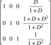 |
| Nonrecursive |  |
aBenedetto et al. [119]. Reproduced by permission of the IEEE.
bNot in referenced table; included here for completeness.
8.12.4 SISO Module
The SISO module37 decoding structures have been characterized in considerable detail by Benedetto et al. [115, 120]. These modules perform maximum a posteriori (MAP) detection processing using a finite‐state trellis decoder and are used in either configuration by appropriately connecting the input and output ports. Figure 8.53 shows an isolated SISO module as a four‐port device with two inputs and outputs denoted, respectively, as λ(c : I), λ(u : I) and λ(c : O), λ(u : O). In the following descriptions of the decoding, the number of iterations is established based on the diminishing improvement in the bit‐error or code block‐error performance and typically 8–20 iterations are used.

FIGURE 8.53 Soft‐in soft‐out processing module.
Benedetto et al. [121]. Reproduced by permission of Elsevier Books.
Depending upon the requirements of the channel coding, the processing complexity can be reduced if M = 2 constituent encoders and SISO decoding modules are used. These simplified implantations follow directly from the M = 2 PCCC and SCCC configurations that are shown in Figures 8.54 and 8.55, respectively. Similarly, the encoding with an arbitrary number (M) of CCs is shown in Figures 8.51 and 8.52, and the corresponding decoding configurations can be inferred from the M = 3 decoding implementations.

FIGURE 8.54 Turbo code implementation (M = 2).

FIGURE 8.55 SCCC code implementation (M = 2).
The TC configuration involves two constituent convolutional encoders and one interleaver and the decoder consists of two SISO modules and one interleaver and deinterleaver as shown in Figure 8.54. In this configuration, there is only one source of received code words available for use by the SISO external observations or inputs λ(c : I). These inputs are obtained directly from the demodulator matched filter; consequently, with PCCC decoding the decoded outputs λ(c : O) is not used. In this case, the SISO1 output λ(u : O) represents the newly formed extrinsic information that is interleaved to form the reliability input λ(u : I) to SISO2. With subsequent iterations, the deinterleaved output from SISO2 is used as the reliability input to SISO1 and the decoding proceeds as described before. Upon completion of the last iteration, the received data is output as shown in Figure 8.54.
The decoding of the SCCC is described in terms of Figure 8.55 using two serially concatenated encoders. In this case, the decoding involves two SISO modules with the input λ(c : I) to the inner SISO corresponding to the demodulator matched filter samples and represents the interleaved symbols received from the channel. The input λ(c : I) to the outer SISO corresponds to the deinterleaved output of the newly formed extrinsic information λ(u : O) from the inner SISO. The newly formed decoded output λ(c : O) of the outer SISO is then interleaved forming the new observations λ(u : I) to the inner SISO. In this case, there is no successive SISO from which to obtain extrinsic information, so the outer SISO input λ(u : I) is set to zero and is not used. At this point, the first iteration is completed and following the last iteration the received data corresponds to the extrinsic information λ(u : O) of outer SISO.
Although the configurations of the PCCC and SCCC implementations are quite different, the processing within the SISO module is very structured with many common algorithms for both codes. The internal processing is based on optimal decoding algorithms for concatenated convolutional codes using the trellis decoding structure. The processing is described in broad terms in the remainder of this section and in detail in Sections 8.12.5 and 8.12.6.
The Bahl–Cocke–Jelinek–Raviv (BCJR) algorithm [122] provides for the MAP decoding of binary convolutional codes using the trellis decoding structure and the SISO processing is a variant of the BCJR algorithm. The MAP algorithm makes symbol‐by‐symbol decisions and, with equal a priori source symbol probabilities, corresponds to the a posteriori probability (APP) algorithm. However, because the SISO module processes a block of information and parity symbols before outputting the symbol decisions, the SISO module uses an additive APP algorithm rather than the MAP algorithm. Divsalar [105] has developed step‐by‐step derivations of the generalized additive APP SISO algorithms for the decoding of turbo, serial, hybrid, and self‐concatenated codes. These derivations compare the multiplicative and additive APP processing within the SISO module for symbol and bit‐level processing. The multiplicative APP forms the product of APPs at each trellis transition and is more computationally complex than the additive APP algorithm, that is based the monotonic property of the logarithm and involves the natural logarithm of the summation of APPs.
The relative computational simplicity in forming the logarithm of the sum of the APPs, however, involves some degree of complexity. The issue is related to the ACS algorithm used to choose the surviving metric at each of the termination states when using the Viterbi algorithm. With the additive APP algorithm, the comparable processing is referred to as an ACS plus correction, or simply the max* (max‐star) operation, defined as

where aji : j = 1, 2 are the exponents of the APPs at state i, L is the number of trellis states, and δ(Δi) is the additive correction term that is stored in a lookup table. The last approximation simply chooses the maximum exponent and results in near‐optimum performance for medium‐to‐high signal‐to‐noise ratios; however, for very low signal‐to‐noise ratios an Eb/No performance loss [123] of 0.5–0.7 dB is encountered; this loss is not insignificant given the overall coding complexity required to approach the channel coding limit. The first approximation in (8.114) involves a table look, based on the additive term in the second equality, and results in nearly the optimum performance when only eight values are stored.
The demodulator matched filter samples (yk,i) represent sufficient statistics that contain all the information required to optimally detect the received information. However, the SISO processing requires that the receiver AGC establish a constant signal level satisfying one of the two following conditions. If the AGC normalizes the signal‐to‐noise ratio so that the additive noise samples (![]() ) represents a zero‐mean, unit‐variance random variables, the sufficient statistics is evaluated as
) represents a zero‐mean, unit‐variance random variables, the sufficient statistics is evaluated as

where ![]() with ck,i = {0,1} and dk,i = {−1,1}. The external observations from the channel are denoted as
with ck,i = {0,1} and dk,i = {−1,1}. The external observations from the channel are denoted as

On the other hand, if the AGC holds the signal level constant at A, such that the signal‐to‐noise ratio is ![]() , then the sufficient statistic is
, then the sufficient statistic is
where ![]() and the external observations from the channel are denoted as
and the external observations from the channel are denoted as

These results apply for BPSK; however, QPSK modulation can be used by considering two independent channels of PSK, each with unit noise variance and this requires dividing (8.116) and (8.118) by two.
Sections 8.12.5 and 8.12.6 describe the iterative decoding details for the parallel and serially concatenated codes involving two SISO modules based on the work of Divsalar [105] and Benedetto and Divsalar [65].
8.12.5 Iterative Decoding of Parallel Concatenated Codes
The computational complexity of the additive APP algorithm is lower than that of the multiplicative APP algorithm; so, for this reason, the additive APP algorithm [117] is described in this section. The description of the PCCC processing is based on Figure 8.54 and the focus is on the bit‐level processing within the SISO module that is commensurate with BPSK and QPSK waveform modulations. To simplify the description of the SISO algorithms, the state metric computation examples are based on a rate 1/2, four‐state binary convolutional encoder; however, the decoding algorithms are expressed in general terms. For example, the code rate38 is rc = p/q where p is the number of information bits; q is the total number of coded bits, including the parity bits; and N is the number of trellis states. For clarity, these parameters are included in the following description. Two major assumptions are made regarding the SISO processing: the channel is memoryless and maps the encoded symbols ck into the matched filter samples yk according to the channel probability density function ![]() ; the encoder is time‐invariant and corresponds to a fixed block code of length K symbols. In this case, with k = 1, …, K, the trellis‐state decoding is completely characterized by each trellis section from state Sk−1(ℓ) to
; the encoder is time‐invariant and corresponds to a fixed block code of length K symbols. In this case, with k = 1, …, K, the trellis‐state decoding is completely characterized by each trellis section from state Sk−1(ℓ) to ![]() . Based on the encoder convention, the decoding starts at state S0(0) and ends at state S0(K) and includes the flush bits required to return the trellis to the known termination state.
. Based on the encoder convention, the decoding starts at state S0(0) and ends at state S0(K) and includes the flush bits required to return the trellis to the known termination state.
The SISO processing is based on the forward and backward recursions through the trellis structure corresponding to the convolutional encoder implementation. The encoder can be implemented as a systematic or nonsystematic code and use recursive encoders, nonrecursive encoders, or both configurations. The recursions take place over the entire code block length of K‐symbols corresponding to the interleaver length;39 however, as mentioned earlier, the SISO processing is based on each trellis section associated with the q‐bit received code symbol. The forward and backward recursions for a trellis section are shown in Figure 8.56. The trellis processing is described using the nomenclature of the referenced authors. The trellis segment for the k‐th input code bit is described in terms of the starting edge SS(e), ending edge SE(e), and the branch metric, ![]() , for edge “e.” These three terms correspond, respectively, to the: source metric, termination metric, and metric update used in Section 8.11.1. To begin the description of the block decoding, the trellis states are initialized as α0(ℓ = 0), β0(ℓ = 0) = 0 and α0(ℓ ≠ 0), β0(ℓ ≠ 0) = −∞ with
, for edge “e.” These three terms correspond, respectively, to the: source metric, termination metric, and metric update used in Section 8.11.1. To begin the description of the block decoding, the trellis states are initialized as α0(ℓ = 0), β0(ℓ = 0) = 0 and α0(ℓ ≠ 0), β0(ℓ ≠ 0) = −∞ with ![]() and
and ![]() initialized to zero.
initialized to zero.

FIGURE 8.56 Example four‐state trellis section showing forward and backward recursions.
8.12.5.1 Forward and Backward Recursions
The forward recursion processing is very similar to that described in Section 8.11.2, with the inclusion of the reliability input λ(u : I). For example, the metric update Δαm in (8.76) is expressed as

and, with the inclusion of the reliability input λ(u : I), the forward recursion branch metric for edge “e” is expressed as

For the forward recursion, the SISO processing computes αk(s) from ![]() where SS(e) points to the starting states that terminate on the ending state
where SS(e) points to the starting states that terminate on the ending state ![]() . In Figure 8.56a, for each ending state there are two starting states, for example, the ending state
. In Figure 8.56a, for each ending state there are two starting states, for example, the ending state ![]() points to the starting states
points to the starting states ![]() and
and ![]() . As in the Viterbi decoding algorithm, a selection algorithm, similar to the ACS algorithm, must be used to determine the surviving metric at each ending state. For the additive APP algorithm, the max*(ai) selection algorithm is used and the surviving metric is computed as
. As in the Viterbi decoding algorithm, a selection algorithm, similar to the ACS algorithm, must be used to determine the surviving metric at each ending state. For the additive APP algorithm, the max*(ai) selection algorithm is used and the surviving metric is computed as

The backward recursion computes βk(s) from ![]() where SS(e) points to the starting states that terminate on the ending state
where SS(e) points to the starting states that terminate on the ending state ![]() . In Figure 8.56b for each ending state, there are two starting states, for example, the ending state
. In Figure 8.56b for each ending state, there are two starting states, for example, the ending state ![]() points to the starting states
points to the starting states ![]() and
and ![]() . In this case, the surviving metric is computed as
. In this case, the surviving metric is computed as

The demodulator matched filter observations λ(c, I) are given by (8.116) and the constants ![]() and
and ![]() are adjusted as required upon completion of each iteration to prevent accumulation overflow. Overflow in path metric computations using fixed‐point processing internal to the SISO must also be considered [124]. The PCCC performance evaluations in this chapter use 32‐bit floating point SISO processing and, to avoid computational overflow, the metric adjustments are made at the completion of each iteration.
are adjusted as required upon completion of each iteration to prevent accumulation overflow. Overflow in path metric computations using fixed‐point processing internal to the SISO must also be considered [124]. The PCCC performance evaluations in this chapter use 32‐bit floating point SISO processing and, to avoid computational overflow, the metric adjustments are made at the completion of each iteration.
For the PCCC implementation, the extrinsic bit information output λ(u : O) for Uk,j ; j = 1, …, p is computed as in (8.123) and the output λ(c : O) is not used.

The data storage requirements involve the forward and backward branch metrics αk, βk, the SISO input data, the interleaver and deinterleaver data, the transition code bits uk,i, and matched filter code‐bit estimates ck,i associated with each branch transition.
8.12.6 Iterative Decoding of Serially Concatenated Convolutional Codes
The serially concatenated code configuration is depicted in Figure 8.55 and the details of the SISO processing and iterative decoding between the two concatenated codes is the subject of this section [118]. Unlike the PCCC decoding algorithm, which only accepts the input bit reliabilities λ(c : I) from the demodulator matched filter, the SCCC decoding algorithm uses the matched filter samples on the first iteration; however, on subsequent iterations the input data reliabilities λ(c : I) are obtained from the deinterleaved extrinsic bit information λ(u : O) from the inner SISO. The outer SISO then computes the extrinsic bit information λ(c : O). In describing the decoding algorithms, the respective inner and outer code rates are p1/q1 and p2/q2, ck(e) represents ck,i(e): i = 1, 2, …, qm for the inner code (m = 1), and uk(e) represents uk,i(e): i = 1, 2, …, pm for the outer code (m = 2). Considering that the p and q input and output bits are binary, represented by {0,1}, the bit‐by‐bit decoding for the M = 2 SCCC code is described as follows.
The max* operation is identical to that defined by (8.114) and the intrinsic input λk(ck,i; I) from the demodulator matched filter samples are identical those described by (8.116). The inner and outer trellises are initialized as described for the PCCC decoding, that is, with α0(ℓ = 0), β0(ℓ = 0) = 0 and α0(ℓ ≠ 0), β0(ℓ ≠ 0) = −∞ with the constants ![]() and
and ![]() initialized to zero. Under these conditions, the inner and outer trellis recursions are computed as follows:
initialized to zero. Under these conditions, the inner and outer trellis recursions are computed as follows:
8.12.6.1 Inner Code Forward and Backward Recursions

and

with the extrinsic bit information for Uk,j: j = 1, 2, … p1 is computed as

8.12.6.2 Outer Code Forward and Backward Recursions

and

with the extrinsic bit information for Ck,j: j = 1, 2, … q2 is computed as

where λk(Ck,j; O) is interleaved and provided to the inner SISO as the input reliabilities λ(ck; I). Upon the final iteration, the output bit reliability Uk,j: j = 1, 2, …, p2 is computed as

8.12.7 PCCC and SCCC Performance
In this section, the bit‐error performance of the PCCCs and SCCCs are examined and compared.40 In the following performance evaluation, the rate 1/3 TC, included in the Consultative Committee for Space Data Systems (CCSDS) multi‐rate TC standard for space telemetry [125], is examined using Monte Carlo simulations. The bit‐error performance is evaluated for various interleaver lengths with four iterations and then with various iterations using an interleaver lengths of 1024 bits. The performance is also evaluated for short messages with interleaver lengths of 296 and 128 bits using 10 iterations. These results highlight the importance of the interleaver length as discussed in Section 8.12.1. In Section 8.12.7.2, the bit‐error performance comparisons between the PCCCs and SCCCs are based on the work of Benedetto, Divsalar, Montorsi, and Pollara. All of the following Monte Carlo performance evaluations correspond to an AWGN channel.
8.12.7.1 Rate 1/3 Turbo Code Performance
The CCSDS [126, 127], recommended TC has selectable code rates of 1/2, 1/3, 1/4, and 1/6 and uses two 16‐state convolutional encoders. The interleaver lengths are also selectable among the following options: 1,784, 3,568, 7,136, 8,920, and 16,384. The encoder including the full complement of code rates is shown in Figure 8.57. The source bits are randomly assigned to the interleaver according to the selected interleaver algorithm. This code is a systematic convolutional encoder with one information‐bit for each output symbol interval, so the delay registers D correspond to the bit interval Tb. The registers are initialized to zero and, following the last of L information bits, the code input switches are changed and four additional clock cycles are executed to terminate the trellis in the zero state. The four additional bits are transmitted and used in the decoder to terminate the decoding trellis in the zero state; consequently, (L + 4)/rc code bits are transmitted to recover the L information bits.

FIGURE 8.57 CCSDS selectable rate turbo code encoder.
CCSDS Blue Book [126]. Reproduced by permission of the Consultative Committee for Space Data Systems (CCSDS).
The generator for the turbo code is G = (g0, g1, g2, g3)T and subgenerators (gi) are listed in Table 8.34 using octal and binary notations. The code consists of recursive generators. The rate 1/2 code is generated by alternately puncturing the connections indicated by the open circles, starting with the encoder b connection, that is, the output of generator g1b is punctured first. The filled circles are fixed connections so there is no puncturing for the code rates 1/3, 1/4, and 1/6. The subgenerator g2b (indicated by the x) is not used in encoder b. The bits in a code symbol are transmitted in the order of the connections (top to bottom) indicated by the circles in Figure 8.57. For example, the information bit is always transmitted first; so, for the rate 1/3 code, the bits associated with the generators (g1a, g1b) are transmitted following the information bit. For the punctured rate 1/2 code, the bit following the information bit in the first symbol is g1a, and in the second symbol is g1b with successive symbols alternating between g1a and g1b. The information and parity bits are sequentially applied to the BPSK waveform modulator and transmitted over the AWGN channel.
TABLE 8.34 Turbo Code Subgenerators for Encoder in Figure 8.57
| Subgenerators | Octala | Binary | Connection |
| g0 | 13 | 100110 | Recursive |
| g1 | 33 | 110110 | Nonrecursive |
| g2 | 52 | 101010 | Nonrecursive |
| g3 | 73 | 111110 | Nonrecursive |
aOctal notation with LSB on the left.
The Monte Carlo simulated performance shown in Figure 8.59 is based on the JPL spread interleaver; the length 2048 JPL spread interleaver data was provided by Divsalar41 as a reference to validate the simulations. The performance of the JPL spread interleaver was also compared to the turbo and random interleavers, discussed in Section 8.12.1, and found to result in slightly improved bit‐error performance. The Monte Carlo bit‐error performance evaluations of the PCCC require considerably longer simulation runs compared to the performance evaluations of convolutional codes using the Viterbi decoding algorithm; this is not surprising in view of the much lower input signal‐to‐noise ratios and the steepness of the bit‐error performance curve. For example, a change in the signal‐to‐noise ratio of one‐tenth of a decibel can result in several orders of magnitude change in the bit‐error performance. In this regard, the signal‐to‐noise ratio (γb) in the simulation is established using (8.115), such that, the peak signal level is
where γb is measure in the bandwidth equal to the bit rate. Using (8.131) results in a zero‐mean, unit‐variance additive noise random variable. As a rule of thumb, the number of frames (Nsim) in the Monte Carlo simulations is given by
where ρ is the error in Pfe; Equation (8.132) is plotted in Figure 8.58 as a function of Pfe for various values of ρ in percent. Based on this rule, a frame‐error probability of Pfe = 10−4 with an 80% accuracy requires a Monte Carlo simulation of 20K frames or code blocks. This rule of thumb is somewhat pessimistic; however, it is useful in establishing a minimum upper limit while monitoring the frame‐error performance to terminate the simulation when the performance improvement appears to saturate. Unless save guards are available to restart the code, it is time‐consuming to underestimate the simulation run times. The following simulations for the 4096‐bit interleaver used about 40M bits for each signal‐to‐noise ratio.

FIGURE 8.58 Rule of thumb for the number of turbo‐like code simulation frames for each signal‐to‐noise ratio.
Figure 8.59a shows the performance using four iterations with interleaver lengths [128] ranging from 256 to 4096 bits. The performance gain, between Pbe = 10−5 and 10−6, in doubling the interleaver length is about 0.1 dB. Figure 8.59b shows the performance for a fixed interleaver length of 1024 bits with iterations ranging from 1 to 10. The diminishing performance gain with additional iterations above 10 is evident in these plots. For example, at Pbe = 10−6 the performance gain between 5 and 10 iteration is about 0.09 dB.

FIGURE 8.59 Rate 1/3 turbo code performance.
An application involving short‐message durations must use commensurately short interleavers, and Figure 8.60 shows the simulated performance using short‐message blocks of 296 and 128 bits. The message bits included a CRC code to reduce the false message acceptance probability. The error floor between Pbe = 10−5 and 10−6 is evident in both codes and, although the 296‐bit interleaver results in a significant coding gain improvement of about 0.6 dB, the error floor is considerably higher than that of the 128‐bit code block. These results highlight the importance of selecting good interleavers that are sufficiently random to provide independent estimates of the a posteriori probabilities for an information symbol given the encoder constraint length and channel memory.

FIGURE 8.60 Rate 1/3 turbo code performance (short messages, iterations = 10).
8.12.7.2 Comparison of PCCC and SCCC Performance
The PCCC bit‐error performance examined in this section is based on the work of Benedetto et al. [100], Benedetto and Montorsi [116], and Benedetto et al. [121]. The performance evaluation involves the rate 1/2, 1/3, 1/4, and 1/15 PCCC implementations corresponding to iterations of 18, 11, 13, and 12 and a common a data block length of 16K bits with 16‐state encoders. The 2/4 rate code is unique, in that it represents the CCs used in the generation of a trellis‐coded modulation (TCM) waveform. For a discussion of the design, implementation, and performance of TCM, refer to Sections 9.4 and 9.5. With TCM the parity‐check redundancy is achieved through additional modulation states so there is no bandwidth expansion. The generator polynomials for the rate 2/4 TCM CCs (denoted as Code A) are listed in Table 8.35.
TABLE 8.35 Rate 2/4 TCM Constraint Length ν = 4, 16‐State Systematic Recursive Constituent Code Generators
| Code | CC | h2 | h1 | h0 | Comments |
| A | CC1 | 33 | 35 | 31 | 16‐state TCM encoders |
| CC2 | 35 | 33 | 31 |
Referring to Section 9.4, the two input bits d2 and d1 of the rate 2/4 code are sequentially selected from the input source data block of N bits. These bits correspond to the systematic output bits ![]() and
and ![]() of the constituent code CC1. The two CCs are evaluated using
of the constituent code CC1. The two CCs are evaluated using

where ![]() are sequentially taken from the independently interleaved block of source data bits. The resulting rate 2/4 systematic encoder results in the four output bits
are sequentially taken from the independently interleaved block of source data bits. The resulting rate 2/4 systematic encoder results in the four output bits ![]() that are mapped to the selected waveform symbol(s) resulting in the rate 1/2 encoder. The generators for the SCCCs denoted as B through E are listed in Table 8.36 using octal notations.
that are mapped to the selected waveform symbol(s) resulting in the rate 1/2 encoder. The generators for the SCCCs denoted as B through E are listed in Table 8.36 using octal notations.
TABLE 8.36 Constituent Code Generators for SCCCs B–E
| Code | Rate | Generatorsa | ||
| CC1 | CC2 | CC3 | ||
| B | 1/2 | |||
| C | 1/3 | |||
| D | 1/4 | |||
| Eb | 1/15 | |||
aOctal notation with the LSB on the left.
bThese generators must be verified (an alternate CC3 parity generator polynomial to 72/13 is 12/13).
The SCCC implementations are based on the encoder and decoder configurations in Figure 8.61 with the CCs obtained from Table 8.33. The output connections of the inner SCCC CC in Figure 8.61b, indicated by the open circles, require puncturing in the order (a,b), starting with connection a and alternating between a and b at the coded symbol rate. The following comparison of the theory, implementation, and bit‐error performance of these codes42 is based on the work of Benedetto et al. [103, 119, 121, 127] and Dolinar et al. [129].
FIGURE 8.61 Selectable rate SCCC encoder.
The performance of the PCCC implementations is shown in Figure 8.62. The performance comparison between the codes is based on comparable complexity in that the codes correspond to 16‐state trellis decoders and the interleaver lengths are identical. Under the indicated conditions, the selection of the code rate is a major decision in achieving a specified signal‐to‐noise condition. However, the performance with longer interleaver block lengths will also result in lower Eb/No operating conditions. These simulation results do not show any Pbe flaring that is customarily associated with a reduction of the slope in the Pbe vs. Eb/No curve. With 16‐state encoders, the flaring usually becomes evident for Pbe below about 10−5 or 10−6 and results in Pbe = 10−15 at Eb/No values of 6 or 7 dB. These determinations are made using theoretical performance bounds based on the number of error events and the weight information sequence [116, 130]. It is noteworthy that SCCCs are less prone to severe flaring. The performance of the rate 2/4 (or 1/2) TCM waveform is somewhat limited to that shown in Figure 8.62 since bandwidth expansion is not an option and the inclusion of additional redundant modulation states has a rapidly diminishing advantage.

FIGURE 8.62 Simulated PCCC code performance.
Benedetto et al. [121]. Reproduced by permission of Elsevier Books.
The performance of the SCCC implementations is shown in Figure 8.63. The performance assessments are based on the identical complexity of the codes in that they each have four‐state trellis decoders with identical the interleaver lengths and iterations. An advantage of the SCCCs is that the SISO processing can run considerably faster than the PCCCs due to the 4 : 1 reduction in the number of states. The SCCC implementations do not show evidence of any Pbe flaring, as seen with four‐state PCCC performance. In comparing the rate 1/4, four‐state PCCC with the rate 1/4, 16‐state PCCC in Figure 8.62, there is a significant advantage in the coding gain using the 16‐state encoder. Furthermore, even though there is no evidence of Pbe flaring in the 16‐state encoder, it is predicted (see Reference 130, figure 15) that flaring is on the verge of occurring at a signal‐to‐noise ratios ![]() dB. In the performance critique of Figure 8.62, it was mentioned that the SCCCs are less prone to severe flaring; however, flaring occurs (see Reference 103, figure 5) with a rate 1/3, four‐state, and 2K interleaver SCCC for Pbe below about 10−8 at
dB. In the performance critique of Figure 8.62, it was mentioned that the SCCCs are less prone to severe flaring; however, flaring occurs (see Reference 103, figure 5) with a rate 1/3, four‐state, and 2K interleaver SCCC for Pbe below about 10−8 at ![]() dB and results in Pbe = 10−15 at
dB and results in Pbe = 10−15 at ![]() . For the PCCC and SCCC implementations the flaring conditions improve with increasing interleaver lengths.
. For the PCCC and SCCC implementations the flaring conditions improve with increasing interleaver lengths.

FIGURE 8.63 Theoretical SCCC performance comparison to rate 1/4 PCCC under identical conditions.
Benedetto et al. [121]. Reproduced by permission of Elsevier Books.
8.13 LDPC CODE AND TPC
The LDPC codes were discovered in 1962 by Gallager [131] and gained in recognition and popularity [132] following the discovery of TCs by Berrou, Glavieux, and Thitimajshima in 1993. Costello and Forney [133] have an excellent paper describing the development of coding theory over this period and through 2007. LDPC codes are block codes, formed from a class of parity‐check codes [134], and specified by a sparse matrix containing binary information‐digits and parity‐check digits denoted as ones; otherwise, the matrix elements are zeros. Using Gallager’s designation (n, j, k), the coded matrix is partitioned into j submatrices, each with k + I rows and n = k(k + I) columns, where n is the code block length. Designating the submatrix rows as i, each row of the first submatrix are filled with k consecutive ones, such that, (i − 1)k, …, ik: i = 1, …, k + I. Upon completion, each row of the first submatrix contains k consecutive ones and each column contains a single one. The remaining j − 1 submatrices are filled with random permutations of the ones in the first submatrix columns, while preserving the condition that the code matrix contains k ones in each row and j ones in each column. LDPC codes constructed in this manner are referred to as regular LDPC codes [135]; however, irregular LDPC codes [136, 137] are not restricted to having an equal number of ones in the code matrix rows and columns as described earlier and, thereby, result in superior performance by increasing the number of check nodes.
The k consecutive digits in the first submatrix correspond to a coded symbol interval consisting of k − j information‐bits and j parity‐bits. The k‐bit symbol is characterized by starting and ending edges much like the symbol edges defined in the trellis decoding of convolutional codes. With this understanding, the code rate of the LDPC code is defined as
The ![]() submatrices contain the known parity‐bit information needed to determine and correct errors in the received LDPC coded data block. The low‐density construction of the code matrix, for large n, results in a minimum distance between nearly all codes of [138]
submatrices contain the known parity‐bit information needed to determine and correct errors in the received LDPC coded data block. The low‐density construction of the code matrix, for large n, results in a minimum distance between nearly all codes of [138]
where δjk is a constant listed in Table 8.37 for several LDPC codes. The minimum distance increases linearly with the code length.
TABLE 8.37 Comparison of δjk for LDPC Code (n, j, k) for Large na
| j | k | Rate rc | δjk | δb |
| 5 | 6 | 1/6 | 0.225 | 0.263 |
| 4 | 5 | 1/5 | 0.210 | 0.241 |
| 3 | 4 | 1/4 | 0.122 | 0.214 |
| 4 | 6 | 1/3 | 0.129 | 0.173 |
| 3 | 5 | 2/5 | 0.044 | 0.145 |
| 3 | 6 | 1/2 | 0.023 | 0.110 |
aGallager [139]. Reproduced by permission of the IEEE.
bThe same ratio of an ordinary parity‐check code of the same rate.
Gallager [131] has also shown that maximum‐likelihood decoding of LDPC codes over a BSC, corresponding to bit‐by‐bit decoding, results in a decoding error probability that decreases exponentially with the block length. However, to take advantage of the performance improvement using iterative decoding before making a hard‐bit decision requires processing of the APP as discussed in Section 8.12.4. The decoding algorithm is formulated in terms of the log‐likelihood ratio, and Gallager’s solution is expressed as

where xd is the received bit in position d of the received sequence {y}, S is the event that xd satisfies the j parity‐check equations associated with position d, Pd is the probability that the transmitted digit xd is 1 conditioned on the received bit in position d with the log‐likelihood ratio LLRd = ln[(1 − Pd)/Pd].43 Defining the log‐likelihood ratio ![]() where Piℓ is defined similarly to Pd for the ℓ′th digit in the i′th first parity‐check set corresponding to second submatrix. The parameters αiℓ and βiℓ represent the sign and magnitude of LLRiℓ and f(βiℓ) is evaluated as
where Piℓ is defined similarly to Pd for the ℓ′th digit in the i′th first parity‐check set corresponding to second submatrix. The parameters αiℓ and βiℓ represent the sign and magnitude of LLRiℓ and f(βiℓ) is evaluated as
Using (8.137), LLRd, and the sign of αiℓ, the evaluation of (8.136) is fairly straightforward and can be computed either serially or in parallel for each input bit. Following the evaluation, if a parity error is detected at xn, the decoder corrects the error based on the sign of (8.136) with the correspondence: LLR ≥ 0 : xn = 0 and LLR < 0 : xn = 1. These corrections are based on hard decisions and apply to the received information and parity bits.44 Using the corrected bits, the process is repeated until a valid code word is detected or after a fixed number of iterations. As an example of the performance, the bit‐error probability of a high code rate IEEE 802.16e‐compliant LDPC code [140, 141] is shown in Figure 8.64a.

FIGURE 8.64 Performance of LDPC and TPC codes.
Gracie et al. [142]. Reproduced by permission of the IEEE.
Prior to the acceptance of LDPC codes, PCs and TPCs [143–146] were in wide use and continue to provide competitive solutions for FEC coding. PCs were introduced by Elias in 1954. The PC is characterized as a serial concatenation of block codes with data permutations and row–column parity‐check bits. For two concatenated block codes, the designations (ni, ki, dmi): i = 1, 2, correspond to ni the length of the code word, ki the number of information bits, and dmi the minimum Hamming distance. With equal parameters, the PC is denoted as45 (n, k, dm)2 where, in general, ![]() , and
, and ![]() . The PC row–column matrix (n1, n2) is formed using submatrix (k1, k2) in the upper‐left portion of (n1, n2) and forming (n2 − k2) row parity‐check bits and (n1 − k1) column parity‐check bits. The resulting PC rate is the product of the individual codes rates. The optimum decoder uses soft decision LLR processing of the rows and columns with iterative decoding to improve the performance. TPC bit‐error rates on the order of 10−11 can be achieved without experiencing the error floor associated with some PCCC designs. The performance of a high code rate IEEE 802.16‐compliant TPC [147] is shown in Figure 8.64b.
. The PC row–column matrix (n1, n2) is formed using submatrix (k1, k2) in the upper‐left portion of (n1, n2) and forming (n2 − k2) row parity‐check bits and (n1 − k1) column parity‐check bits. The resulting PC rate is the product of the individual codes rates. The optimum decoder uses soft decision LLR processing of the rows and columns with iterative decoding to improve the performance. TPC bit‐error rates on the order of 10−11 can be achieved without experiencing the error floor associated with some PCCC designs. The performance of a high code rate IEEE 802.16‐compliant TPC [147] is shown in Figure 8.64b.
LDPC code and TPC are processing efficient high‐rate codes with performance approaching within a few tenths of a decibel of the channel capacity. On the other hand, Chung et al. [148] demonstrated that a rate 1/2 irregular LDPC code with block length of 107 approaches the channel capacity for binary codes to within 0.04 dB achieving Pbe = 10−6 at Eb/No = 0.19 dB. The long interleaver lengths required for low‐rate LDPC code and TPC are restrictive for applications requiring low message latency. However, with parallel processing the decoding speeds can accommodate tens of Mbps data rates. These codes are also better suited for short messages, on the order of 256 bits or less, than concatenated convolution codes with performance limited by the noise floor.
The preceding description of LDPC coding is based on Gallager’s original publication on low‐density parity‐check encoding and decoding and significant advances have been made since the mid‐1990s when his work was recognized as providing competitive solutions to the need for low Eb/No, nearly error‐free, communication systems. The advances in high‐speed, high‐memory, and low‐power signal processing hardware were also a major motivation. In this regard, the vast amount of current literature on FEC coding, including the LDPC code and TPC should be consulted for the latest innovations, for example, the special issue of the IEEE Proceedings [149] contains a wealth of information, including many references, on a variety of FEC coding techniques, designs, and algorithms. TC synchronization [150, 151] is a major consideration in the system design and synchronization requirements for various standard FEC codes are detailed in the CCSDS specifications [152]. The impact on the performance through channels with memory [153] is another important consideration.
8.14 BOSE‐CHAUDHURI‐HOCQUENGHEM CODES
The binary BCH codes [34, 37] are block codes of length N containing K information bits with an error correction capability of t bit or symbol errors; in the following discussions, the binary BCH codes are denoted as (N, K, t); on occasions, the notation (N, K, t)m is used where m determines the number of bits or symbols in the code block given by N = 2m − 1. Binary BCH codes are generated over the GF(2m) with the binary polynomial coefficients in GF(2). The code polynomials are related to the parameters N, K, t, and m as and the number of parity bits satisfies the condition N − K ≤ mt.46 The BCH codes will correct all combinations of t errors for t ≤ (d − 1)/2 where d is the minimum distance of the code. These parameters are listed in Table 8.38 [154] for binary BCH codes generated over GF(2m) for 3 ≤ m ≤ 10 corresponding to codes of length 7–1023. The parameter tbin = t is used to emphasize the binary BCH code error correction capability. However, the parameters N and K also apply to the nonbinary BCH RS codes with 2m‐ary symbols generated over GF(2m). The nonbinary RS code will correct any combination of trs = t = ![]() m‐bit symbol‐errors or less; the fourth column in Table 8.38 tabulates trs for the RS code.
m‐bit symbol‐errors or less; the fourth column in Table 8.38 tabulates trs for the RS code.
TABLE 8.38 BCH Code Parameters Generated by Primitive Elementsa,b
| N | K | tbin | trs | N | K | tbin | trs | N | K | tbin | trs |
| 7 | 4 | 1 | 1 | 255 | 163 | 12 | 46 | 511 | 277 | 28 | 117 |
| 15 | 11 | 1 | 2 | 155 | 13 | 50 | 268 | 29 | 121 | ||
| 7 | 2 | 4 | 147 | 14 | 54 | 259 | 30 | 126 | |||
| 5 | 3 | 5 | 139 | 15 | 58 | 250 | 31 | 130 | |||
| 31 | 26 | 1 | 2 | 131 | 18 | 62 | 241 | 36 | 135 | ||
| 21 | 2 | 5 | 123 | 19 | 66 | 238 | 37 | 136 | |||
| 16 | 3 | 7 | 115 | 21 | 70 | 229 | 38 | 141 | |||
| 11 | 5 | 10 | 107 | 22 | 74 | 220 | 39 | 145 | |||
| 6 | 7 | 12 | 99 | 23 | 78 | 211 | 41 | 150 | |||
| 63 | 57 | 1 | 3 | 91 | 25 | 82 | 202 | 42 | 154 | ||
| 51 | 2 | 6 | 87 | 26 | 84 | 193 | 43 | 159 | |||
| 45 | 3 | 9 | 79 | 27 | 88 | 184 | 45 | 163 | |||
| 39 | 4 | 12 | 71 | 29 | 92 | 175 | 46 | 168 | |||
| 36 | 5 | 13 | 63 | 30 | 96 | 166 | 47 | 172 | |||
| 30 | 6 | 16 | 55 | 31 | 100 | 157 | 51 | 177 | |||
| 24 | 7 | 19 | 47 | 42 | 104 | 148 | 53 | 181 | |||
| 18 | 10 | 22 | 45 | 43 | 105 | 139 | 54 | 186 | |||
| 16 | 11 | 23 | 37 | 45 | 109 | 130 | 55 | 190 | |||
| 10 | 13 | 26 | 29 | 47 | 113 | 121 | 58 | 195 | |||
| 7 | 15 | 28 | 21 | 55 | 117 | 112 | 59 | 199 | |||
| 127 | 120 | 1 | 3 | 13 | 59 | 121 | 103 | 61 | 204 | ||
| 113 | 2 | 7 | 9 | 63 | 123 | 94 | 62 | 208 | |||
| 106 | 3 | 10 | 85 | 63 | 213 | ||||||
| 99 | 4 | 14 | 511 | 502 | 1 | 4 | 76 | 85 | 217 | ||
| 92 | 5 | 17 | 493 | 2 | 9 | 67 | 87 | 222 | |||
| 85 | 6 | 21 | 484 | 3 | 13 | 58 | 91 | 226 | |||
| 78 | 7 | 24 | 475 | 4 | 18 | 49 | 93 | 231 | |||
| 71 | 9 | 28 | 466 | 5 | 22 | 40 | 95 | 235 | |||
| 64 | 10 | 31 | 457 | 6 | 27 | 31 | 109 | 240 | |||
| 57 | 11 | 35 | 448 | 7 | 31 | 28 | 111 | 241 | |||
| 50 | 13 | 38 | 439 | 8 | 36 | 19 | 119 | 246 | |||
| 43 | 14 | 42 | 430 | 9 | 40 | 10 | 127 | 250 | |||
| 36 | 15 | 45 | 421 | 10 | 45 | ||||||
| 29 | 21 | 49 | 412 | 11 | 48 | 1023 | 1013 | 1 | 5 | ||
| 22 | 23 | 52 | 403 | 12 | 54 | 1003 | 2 | 10 | |||
| 15 | 27 | 56 | 394 | 13 | 58 | 993 | 3 | 15 | |||
| 8 | 31 | 59 | 385 | 14 | 63 | 983 | 4 | 20 | |||
| 255 | 247 | 1 | 4 | 376 | 15 | 67 | 973 | 5 | 25 | ||
| 239 | 2 | 8 | 367 | 16 | 72 | 963 | 6 | 30 | |||
| 231 | 3 | 12 | 358 | 18 | 76 | 953 | 7 | 35 | |||
| 233 | 4 | 11 | 349 | 19 | 81 | 943 | 8 | 40 | |||
| 215 | 5 | 20 | 340 | 20 | 85 | 933 | 9 | 45 | |||
| 207 | 6 | 24 | 331 | 21 | 90 | 923 | 10 | 50 | |||
| 199 | 7 | 28 | 322 | 22 | 94 | 913 | 11 | 55 | |||
| 191 | 8 | 32 | 313 | 23 | 99 | 903 | 12 | 60 | |||
| 187 | 9 | 34 | 304 | 25 | 103 | 893 | 13 | 65 | |||
| 179 | 10 | 38 | 295 | 26 | 108 | 883 | 14 | 70 | |||
| 171 | 11 | 42 | 286 | 27 | 112 | 873 | 15 | 75 | |||
| N | K | tbin | trs | K | tbin | trs | K | tbin | trs | ||
| 1023 | 863 | 16 | 80 | 573 | 50 | 225 | 278 | 102 | 372 | ||
| 858 | 17 | 82 | 563 | 51 | 230 | 268 | 103 | 377 | |||
| 848 | 18 | 87 | 553 | 52 | 235 | 258 | 106 | 382 | |||
| 838 | 19 | 92 | 543 | 53 | 240 | 248 | 107 | 387 | |||
| 828 | 20 | 97 | 533 | 54 | 245 | 238 | 109 | 392 | |||
| 818 | 21 | 102 | 523 | 55 | 250 | 228 | 110 | 397 | |||
| 808 | 22 | 107 | 513 | 57 | 255 | 218 | 111 | 402 | |||
| 798 | 23 | 112 | 503 | 58 | 260 | 208 | 115 | 407 | |||
| 788 | 24 | 117 | 493 | 59 | 265 | 203 | 117 | 410 | |||
| 778 | 25 | 122 | 483 | 60 | 270 | 193 | 118 | 415 | |||
| 768 | 26 | 127 | 473 | 61 | 275 | 183 | 119 | 420 | |||
| 758 | 27 | 132 | 463 | 62 | 280 | 173 | 122 | 425 | |||
| 748 | 28 | 137 | 453 | 63 | 285 | 163 | 123 | 430 | |||
| 738 | 29 | 142 | 443 | 73 | 290 | 153 | 125 | 435 | |||
| 728 | 30 | 147 | 433 | 74 | 295 | 143 | 126 | 440 | |||
| 718 | 31 | 152 | 423 | 75 | 300 | 133 | 127 | 445 | |||
| 708 | 34 | 157 | 413 | 77 | 305 | 123 | 170 | 450 | |||
| 698 | 35 | 162 | 403 | 78 | 310 | 121 | 171 | 451 | |||
| 688 | 36 | 167 | 393 | 79 | 315 | 111 | 173 | 456 | |||
| 678 | 37 | 172 | 383 | 82 | 320 | 101 | 175 | 461 | |||
| 668 | 38 | 177 | 378 | 83 | 322 | 91 | 181 | 466 | |||
| 658 | 39 | 182 | 368 | 85 | 327 | 86 | 183 | 468 | |||
| 648 | 41 | 187 | 358 | 86 | 332 | 76 | 187 | 473 | |||
| 638 | 42 | 192 | 348 | 87 | 337 | 66 | 189 | 478 | |||
| 628 | 43 | 197 | 338 | 89 | 342 | 56 | 191 | 483 | |||
| 618 | 44 | 202 | 328 | 90 | 347 | 46 | 219 | 488 | |||
| 608 | 45 | 207 | 318 | 91 | 352 | 36 | 223 | 493 | |||
| 598 | 46 | 212 | 308 | 93 | 357 | 26 | 239 | 498 | |||
| 588 | 47 | 217 | 298 | 94 | 362 | 16 | 147 | 503 | |||
| 578 | 49 | 222 | 288 | 95 | 367 | 11 | 255 | 506 | |||
aThe shaded parameters result in approximate code rates of 1/2 for the given N.
bPeterson and Weldon [154]. Reproduced by permission of The MIT Press.
A more extensive list of binary cyclic codes of odd length is given by Peterson and Weldon [155] in terms of the parameters N, K, d, dBCH and the roots of the generating polynomials. In this case, d is the true minimum distance of the code and dBCH the minimum distance guaranteed by the BCH bound. The extensive table of results is accredited to Chen [156] and applies to all binary cyclic codes of odd length or degrees ≤65. The results in Table 8.38 represent the codes of a given length for which dxmax(dBCH).
Section 8.14.1 focuses on binary BCH codes with the intent of introducing some basic concepts for examining the more powerful error‐correction capabilities of nonbinary, or q‐ary BCH, codes where the q‐ary symbols are generated over the GF(q). In particular, the nonbinary case is specialized to the RS code for which q = 2m.
8.14.1 Binary BCH Codes
This section briefly reviews binary BCH codes as an introduction to RS codes discussed in Section 8.14.2. To this end, the following introduces the GF(2) involving binary data di ∈ {0,1}. The set of elements α forms a field [157] with respect to addition and multiplication, if the set is closed with respect to addition and multiplication, the distributive law applies, and it contains a zero and unit element. The key to the generation of the field elements over GF(2) is that the generator, or primitive polynomial p(x), has binary coefficients47 {0,1}. The field element for which p(α) = 0 is referred to as the primitive element. Furthermore, the primitive polynomials for which p(α) = 0 are irreducible polynomials, that is, p(x) of degree m are not divisible by any other polynomial of degree m′: 0 < m′ < m ; this ensures that the field is closed.
Construction of the elements over GF(2) is best described by the following example using m = 3 and the known primitive polynomial p(x) = x3 + x + 1. Using the primitive polynomial, all of the distinct 23 symbols of the code are generated in terms of the primitive element α as shown in Table 8.39.
TABLE 8.39 Construction of the GF(23) Using p(x) = x3 + x + 1 [f(x) = b2x2 + b1x + b0]
| Elements | Reduction over Coefficient Field GF(2) | b2 b1 b0 | Integer |
| 0 | 0 0 0 | 0 | |
| 1 | 0 0 1 | 1 | |
| α | 0 1 0 | 2 | |
| α2 | 1 0 0 | 4 | |
| α3 | α + 1 | 0 1 1 | 3 |
| α4 | αα3 = α(α + 1) = α2 + α | 1 1 0 | 6 |
| α5 | αα4 = α(α2 + α) = α2 + α + 1 | 1 1 1 | 7 |
| α6 | αα5 = α(α2 + α + 1) = α2 + 1 | 1 0 1 | 5 |
| α7 | αα6 = α(α2 + 1) = 1 | 0 0 1 | 1 |
In the second column of Table 8.39, the primitive polynomial provides the key equality p(α) = α3 + α + 1 = 0 from which α3 = α + 1 is determined. Furthermore, addition and subtraction are indistinguishable, multiplication is performed by adding the exponents, and the field is closed, that is, α7 = 1. The primitive element of the field is the unit element so the set of elements ![]() form the 2m unique elements of the field. As mentioned earlier, the operations of addition and subtraction are the same in GF(2) with the special case αn ± αn = 0 : 0 ≤ n ≤ m − 1; these properties are a direct result of the modulo‐2 addition of the binary coefficients bn. Multiplication is performed simply by adding the exponents as αnαn′ = αn+n′.
form the 2m unique elements of the field. As mentioned earlier, the operations of addition and subtraction are the same in GF(2) with the special case αn ± αn = 0 : 0 ≤ n ≤ m − 1; these properties are a direct result of the modulo‐2 addition of the binary coefficients bn. Multiplication is performed simply by adding the exponents as αnαn′ = αn+n′.
Primitive polynomials are difficult to determine; however, Table 8.40 provides a list, for m = 3 through 10; these polynomials are also applicable to 8‐ary through 1024‐ary RS codes discussed in Section 8.14.2. More extensive tables of primitive polynomials are provided by Peterson and Weldon [155], from which Table 8.40 is compiled, and by Lin [37], Peterson [58], and Marsh [158].
TABLE 8.40 Primitive Polynomials for GF(2m) for m = 2–10a
| m | p(x) |
| 2 | x2 + x + 1 |
| 3 | x3 + x + 1 |
| 4 | x4 + x + 1 |
| 5 | x 5 + x2 + 1 |
| 6 | x6 + x + 1 |
| 7 | x7 + x3 + 1 |
| 8 | x8 + x4 + x3 + x2 + 1 |
| 9 | x9 + x4 + 1 |
| 10 | x10 + x3 + 1 |
aPartial list from Reference 155.
Binary BCH codes are defined for any positive integers m and t with the following properties:
- Block length n = 2m − 1
- Parity‐check bits n − k ≤ mt
- Minimum distance d ≥ 2t + 1
The binary BCH code is denoted as a (n, k, t) t‐error correcting code, where t or less errors can be corrected in any block of n bits, where (n − k)/m ≤ t ≤ (d − 1)/2. There is no easy way to evaluate the value n − k that satisfies the equality mt = (n − k); however, the values of t are tabulated in the third column of Table 8.38 as tbin.
The generator polynomial of a, t‐error‐correcting, binary BCH code is defined as the least common multiple (LCM) of the minimum polynomials48 mi(x) : i = 1, 3, 5, …, 2t − 1, expressed as
Comparing (8.151), the expression for computing the generator polynomials for nonbinary RS codes, with (8.138), it appears evident that determining the generator polynomials for binary BCH codes is considerably more difficult. The details for determining the minimum polynomials for the primitive element in GF(2) and the generator polynomial g(x) are discussed by Lin [159], Lin and Costello [160], and Peterson and Walden [34]. Peterson and Walden (Appendix C) provide tables of irreducible polynomials over GF(2) in which the minimum polynomials are identified. Michelson and Levesque [63] provide succinct descriptions of these topics with an explanation of the method for determination of the minimum polynomials from Peterson’s table. The generator polynomials for primitive binary BCH codes, tabulated by Stenbit [161], are listed in Appendix 8B.
Referring to Appendix 8B, the generator for the length n = 15, t = 2 error‐correcting (15,7,2) binary BCH code, in octal notation, is (721) and, considering the binary coefficients gi = {1,0}, the generator is computed as

The generator is implemented as shown in Figure 8.66 for the RS code; however, the generator weights gi corresponding to the coefficients of (8.139) are equal to binary one.
The decoding involves the following three principal decoding computations:
- Error syndrome calculation
- Error location polynomial calculations
- Error location calculation
The computation of the error values, required for the RS code, is not required because the error correction simply involves changing the binary coefficient at the calculated error location. There are several techniques, including the Berlekamp algorithm, that are used in the decoding computations for the binary BCH codes; these techniques are discussed by several authors [37, 58, 160, 162–165]. The following sections focus on the decoding of the binary BCH codes with the major emphasis on the decoding of M‐ary RS codes using the Berlekamp algorithm. The procedures for finding and correcting the errors in the binary BCH code are identified by evaluating the t rows of Table 8.41 as described by Lin [166]. The table is initiated as shown and the rows are completed iteratively, as described by the following algorithm, in the process of determining the error location polynomial.
TABLE 8.41 Binary BCH Iterative Algorithm for Determining the Error Location Polynomiala
| υ | συ(x) | dυ | ℓυ | |
| −1/2 | 1 | 1 | 0 | −1 |
| 0 | 1 | S1 | 0 | 0 |
| 1 | ||||
| … | ||||
| t |
aLin [166]. Reproduced by permission of Pearson Education, Inc., New York, NY.
Table 8.41 is filled out using the following algorithm. Given the previous row υ, the υ + 1 row is determined as
if (dυ = 0) thenelseFind another row, such that the last column

is the largest value with, and then compute:
end if: the degree of
and
where theare the coefficients of the polynomial
The polynomial σt(x) in the last row of Table 8.41 is the error location polynomial; however, if it has degree greater than t, the errors cannot be located and corrected.
8.14.2 RS Codes
The RS code is a subclass of nonbinary BCH codes that have excellent burst‐ and random error correcting properties. In general, the M‐ary RS code has a code or block length of N = M − 1 symbols where each symbol is composed of an M‐ary symbol alphabet. Referring to the number of information symbols as K < N, the M‐RS code is designated as a (N, K) code. The code rate is defined as rc = K/N. The error‐free correction capability of the RS code is t = (N − K)/2 symbols, that is, any combination of symbol errors equal to or less than one‐half the number of parity symbols can be corrected. In the following discussions, the notation (N, K, t) is used to explicitly identify the error‐correction capability being considered. The minimum distance of the RS code is ![]() . In the event that the decoder fails to correct the received symbol errors, additional processing can be performed by using symbol erasures to correct up to
. In the event that the decoder fails to correct the received symbol errors, additional processing can be performed by using symbol erasures to correct up to ![]() symbol errors where e is the number of symbols that are erased. The decision as to which symbols to erase must be made on the basis of a maximum‐likelihood rule at the symbol detection processor output; noisy threshold margins will influence the erasure selections. The code symbols most commonly used in the implementation of the RS code are taken from the GF(2m) where M = 2m. The notation (N, K, t)m is used to identifying the underlying code structure. This is a particularly useful notation when dealing with shortened codes with N < M − 1 that may lead to confusion as to the applicable GF. Several references are given in the following sections in which the details of GF arithmetic can be found. The RS code characteristics are summarized in Table 8.42.
symbol errors where e is the number of symbols that are erased. The decision as to which symbols to erase must be made on the basis of a maximum‐likelihood rule at the symbol detection processor output; noisy threshold margins will influence the erasure selections. The code symbols most commonly used in the implementation of the RS code are taken from the GF(2m) where M = 2m. The notation (N, K, t)m is used to identifying the underlying code structure. This is a particularly useful notation when dealing with shortened codes with N < M − 1 that may lead to confusion as to the applicable GF. Several references are given in the following sections in which the details of GF arithmetic can be found. The RS code characteristics are summarized in Table 8.42.
TABLE 8.42 Summary of M‐ary Reed–Solomon Code Characteristics
| Parameter | Symbols | Bits |
| Block length (N) | M − 1 | m(M − 1) |
| Bits/symbol (m) | — | log2(M) |
| Information | K | mK |
| Parity | N − K | m(N − K) |
| Error correction | ||
| Without erasures (t) | (N − K)/2 | m(N − K)/2 |
| With erasures (t′) | (2t − e)/2 | m(2t − e)/2 |
| Min. distance (dmin) | 2t + 1 | — |
In the following sections, the message format and encoding requirements are reviewed for a general M‐ary RS encoder. Of particular interest is the development of the encoder vector notation from the transmitted sequence. The vector notation represents the encoded message as a polynomial upon which the decoding algorithms are performed and is not an implicit function of time. Also the concept of shortened codes is introduced for which a specific example of a (24,12) code is given. The following discussion focuses on the processing requirements without the use of erasures; the processing requirement with erasures is discussed in Section 8.14.2.3. In either case, with or without erasures, the four principal decoding computations involve:
- Error syndrome calculation
- Error location polynomial calculations
- Error location calculation
- Error value calculations
The concluding sections outline a computer simulation code for all of the required processing for both the encoder and decoder. This chapter concludes with a discussion of several theoretical and simulated performance results. The performance is characterized in terms of the bit‐error probability dependence on the signal‐to‐noise ratio as measured in the symbol and information‐bit bandwidths.
8.14.2.1 Encoder Processing
This section relates the source data information or message sequence to the sequence of encoded symbols including the parity symbols. The parity symbols are appended to the message to form a systematic M‐ary RS coded sequence. The relationship between the time‐dependent transmitted sequence and the notion of a code vector generated from elements of the GF(2m) is discussed. Also, the generation of shortened forms of the underlying or parent (N, K) code is discussed.
Binary data comprising the source message is collected in a block of mK bits and taken m at a time to form K message symbols. Each symbol forms a 2m‐ary vector that is represented as an element in the GF having a primitive polynomial p(α) where α is called the “primitive element.” Therefore, each nonzero message symbol can be represented as a power of α such that
where n = i modulo‐(2m − 1) and i is any integer. The complete set consists of the 2m elements ![]() .
.
Most of the simulation examples provided in the following sections are based on the 64‐ary RS code generated over GF(26) and the corresponding set of elements are listed in Table 8.43. These elements form the basis upon which the encoding and decoding operations are performed and serve to illustrate the algebraic properties of GFs. The nonzero elements of GF(26) are generated from the primitive polynomial
with ![]() . The binary values are assigned, from left to right, as (b0, b1, b2, b3, b4, b5) where b0 is the LSB. The LSB is taken first‐in‐time from the data source, or parity generator, and is transmitted first‐in‐time. The relationship between the binary bits and the primitive element α for a typical symbol is
. The binary values are assigned, from left to right, as (b0, b1, b2, b3, b4, b5) where b0 is the LSB. The LSB is taken first‐in‐time from the data source, or parity generator, and is transmitted first‐in‐time. The relationship between the binary bits and the primitive element α for a typical symbol is

TABLE 8.43 Binary and Integer Equivalents of Field Elements in GF(26) [f(x) = b5x5 + b4x4 + b3x3 + b2x2 + b1x + b0]
| Symbol | Binary | Integer | Symbol | Binary | Integer |
| 0 | 000000 | 0 | α31 | 100101 | 37 |
| α0 | 000001 | 1 | α32 | 001001 | 9 |
| α1 | 000010 | 2 | α33 | 010010 | 18 |
| α2 | 000100 | 4 | α34 | 100100 | 36 |
| α3 | 001000 | 8 | α35 | 001011 | 11 |
| α4 | 010000 | 16 | α36 | 010110 | 22 |
| α5 | 100000 | 32 | α37 | 101100 | 44 |
| α6 | 000011 | 3 | α38 | 011011 | 27 |
| α7 | 000110 | 6 | α39 | 110110 | 54 |
| α8 | 001100 | 12 | α40 | 101111 | 47 |
| α9 | 011000 | 24 | α41 | 011101 | 29 |
| α10 | 110000 | 48 | α42 | 111010 | 58 |
| α11 | 100011 | 35 | α43 | 110111 | 55 |
| α12 | 000101 | 5 | α44 | 101101 | 45 |
| α13 | 001010 | 10 | α45 | 011001 | 25 |
| α14 | 010100 | 20 | α46 | 110010 | 50 |
| α15 | 101000 | 40 | α47 | 100111 | 39 |
| α16 | 010011 | 19 | α48 | 001101 | 13 |
| α17 | 100110 | 38 | α49 | 011010 | 26 |
| α18 | 001111 | 15 | α50 | 110100 | 52 |
| α19 | 011110 | 30 | α51 | 101011 | 43 |
| α20 | 111100 | 60 | α52 | 010101 | 21 |
| α21 | 111011 | 59 | α53 | 101010 | 42 |
| α22 | 110101 | 53 | α54 | 010111 | 23 |
| α23 | 101001 | 41 | α55 | 101110 | 46 |
| α24 | 010001 | 17 | α56 | 011111 | 31 |
| α25 | 100010 | 34 | α57 | 111110 | 62 |
| α26 | 000111 | 7 | α58 | 111111 | 63 |
| α27 | 001110 | 14 | α59 | 111101 | 61 |
| α28 | 011100 | 28 | α60 | 111001 | 57 |
| α29 | 111000 | 56 | α61 | 110001 | 49 |
| α30 | 110011 | 51 | α62 | 100001 | 33 |
Because of this assignment of the LSB, it is necessary in the simulation to reverse the binary symbol to accommodate the vector processing as defined throughout the literature and used in the following sections.
In completing Table 8.43, it is noted that the first m − 1 powers of α are simply evaluated as ![]() , i = 0, 1, …, m − 1 and αm is evaluated directly from the solution of the primitive polynomial as
, i = 0, 1, …, m − 1 and αm is evaluated directly from the solution of the primitive polynomial as ![]() . Subsequent powers are determined by repeated multiplication by α and subsequent reduction using the first m powers previously evaluated. Multiplication (division) over GF(2m) is performed simply by adding (subtracting), modulo‐(2m − 1), the exponents of α, that is,
. Subsequent powers are determined by repeated multiplication by α and subsequent reduction using the first m powers previously evaluated. Multiplication (division) over GF(2m) is performed simply by adding (subtracting), modulo‐(2m − 1), the exponents of α, that is, ![]() and
and ![]() . Addition over GF(2m) is performed by forming the binary representations of the terms being added and summing the corresponding coefficients modulo‐2; this is the same as performing an exclusive‐or on the corresponding binary elements. For example, referring to Table 8.43 and (8.140),
. Addition over GF(2m) is performed by forming the binary representations of the terms being added and summing the corresponding coefficients modulo‐2; this is the same as performing an exclusive‐or on the corresponding binary elements. For example, referring to Table 8.43 and (8.140), ![]() , noting that,
, noting that, ![]() .
.
Figure 8.65 depicts an arbitrary message symbol from a data source with each symbol composed of m source data bits. The collection of K source symbols forms the RS code block duration.

FIGURE 8.65 Relationship between source message bits, symbols, and code block.
The message sequence is described as

and the parity sequence is described as

where
and

For the systematic‐code format, the parity is simply appended to the message sequence and results in the transmitted code sequence expressed as
It is convenient to represent the transmitted sequence as an N‐dimensional code vector by making the substitution49 x−n = d(t − nT) which gives

Applying the common coefficient notation
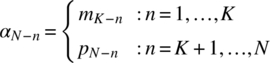
to each summation in (8.148) and multiplying both sides by XN−1 result in the simplified expression

where the first N − K terms represent the parity information and the remaining K terms represent the unaltered message information.
It is important to keep in mind the apparent reversal of the message and parity information symbols between the sequence notation of (8.147) and the vector notation of (8.150). In both cases, the message symbols are transmitted first and the first message symbol into the receiver corresponds to the coefficient of the highest order (N − 1) term of r(X). The expression for r(X) given by (8.150) presupposes an encoder implementation that stores the sequence prior to the encoding and transmission. This is not required, however, and r(X) can be generated without delay between the data source and modulator as shown in Figure 8.66.

FIGURE 8.66 Reed–Solomon encoder.
The tap weights, gn, of the parity generator are determined from the coefficients of the generator polynomial g(X). For the t‐error correcting RS code, g(X) is expressed as

where ![]() and
and ![]() .
.
This description of the generator polynomial is not unique and more in‐depth discussions can be found in the literature [37, 157, 158, 164, 167]. All of these operations must be performed in accordance with the algebraic rules of the GF(2m). As in the previous discussion of mn and pn, gn is also an element of the GF for which
Although the basic M‐ary RS code for which M = 2m is defined for N = M − 1, a shortened code for N < M − 1 can be easily implemented by considering the first message symbols mn: n = N, …, M − 1 to be zero. As is evident from Figure 8.66, these leading message symbols will not contribute to the parity information. For example, the shortened (32,20) 64‐ary RS code assumes that the code vector is expressed as
The shortened RS codes are denoted as (N′, K′, t′)m codes that are derived from the parent (N, K, t)m code by reducing the N and K symbols by a constant integer I < K. The resulting shorted code corresponds to N′ = N − I and K′ = K − I. Although the symbol‐error correction capability remains the same, that is, t′ = t, the code rate of the shortened code is
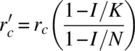
so that, for I > 0, ![]() .
.
8.14.2.2 Decoder Processing without Erasures
When errors, introduced by the transmission media, are added to the transmitted code vector r(X) the resulting received vector is expressed as
The first operation of the receiver decoder is to compute the error syndrome to determine the existence of errors. For the RS codes, the syndrome is a 2t‐dimensional vector given by

When S(X) ≠ 0, it is concluded that errors have occurred in the received data and that additional processing must be performed to determine their locations and magnitudes. The components Si are examined individually to determine the existence of an error condition. These components are given by

where ![]() are the coefficients of the received vector. Whenever
are the coefficients of the received vector. Whenever ![]() , the message block is assumed to be received without errors; otherwise, an error condition is declared. The operations involved in computing Si are referred to as the parity‐check calculations.
, the message block is assumed to be received without errors; otherwise, an error condition is declared. The operations involved in computing Si are referred to as the parity‐check calculations.
In the event of υ ≤ t symbol errors, there exists a set of unique nonzero error location numbers (Xℓ) and error value numbers (Yℓ) that are related to the syndrome components by

The problem in solving the nonlinear equations (8.158) for Xℓ and Yℓ was the major task facing algebraic coding theorists and the major task facing hardware or software engineers is to efficiently implement the resulting algorithms. The following development follows closely that given by Berlekamp.50
When υ ≤ t errors occur a set of elementary symmetric functions, σℓ, are defined by the equations

where the elementary symmetric functions are related to the error syndrome components by the linear equations51

Berlekamp developed an iterative procedure for solving this set of linear equations for the elementary symmetric functions and Lin presents a simplified outline of the algorithms. The procedure involves completing Table 8.44 after initialization of the first two rows as shown. In Table 8.44, Si is the error syndrome computed previously and completion of the table, given the υ‐th row, is accomplished as follows:
if (dυ = 0), thenelseFind row, such that the last column

is the largest value with, and then compute:
endif
where theare the coefficients of the polynomial
TABLE 8.44 Iterative Algorithm Table for the Error Location Polynomiala
| υ | συ(x) | dυ | ℓυ | |
| −1 | 1 | 1 | 0 | −1 |
| 0 | 1 | S1 | 0 | 0 |
| 1 | ||||
| … | ||||
| 2t |
aLin [166]. Reproduced by permission of Pearson Education, Inc., New York, NY.
Finding the row such that υ′ < υ under the indicated conditions requires completing 2t rows in Table 8.44 and the polynomial σ2t(x) in the last row is the error location polynomial. If the degree of this polynomial is greater than 2t, the errors cannot be located and corrected.
Upon successful completion of Table 8.44, the resulting polynomial σ2t(x) is the required error location polynomial. Therefore, having solved for the elementary symmetric functions (σℓ), the error locations numbers are determined as follows. The right‐hand side of (8.159) is referred to as the error location polynomial, and it follows from the left‐hand side of (8.159) that any valid error location number ![]() is related to the roots of this polynomial. The roots form a subset of the GF(2m) field elements given by
is related to the roots of this polynomial. The roots form a subset of the GF(2m) field elements given by
from which the error location numbers are given by
This is equivalent to identifying the error location in terms of the power n of Xn given in (8.150). Therefore, the location of the received symbol αn that is in error is given by the coefficients of Xn in the received vector where n = N − i.
The terminology used here is consistent with that used by Berlekamp. Peterson [58], however, defines the error locations as being the reciprocal of the error location numbers. The difference arises because of the form of (8.159), which Peterson expresses as

The location numbers are determined simply by substituting each element of GF(2m), except zero, into (8.159) and taking those values that are roots.
Having computed the error locations, the error values (Yℓ) are determined from (8.158), which is linear in Yℓ. For the binary BCH codes, the received bits found to be in error are simply inverted to give the corrected information. Determining the error values for the nonbinary BCH codes, however, is considerably more involved. The error values are expressed as

where W(X) is referred to as the error evaluation polynomial and can be expressed in the form

where the coefficients are given by

where So = 1, ![]() are the previously computed error syndromes, and σj are the elementary symmetric functions. An alternate procedure for computing the error values when with erasures is discussed in Section 8.14.2.3.
are the previously computed error syndromes, and σj are the elementary symmetric functions. An alternate procedure for computing the error values when with erasures is discussed in Section 8.14.2.3.
8.14.2.3 Decoder Processing with Erasures
As outlined in this section, the processing requirements with erasures follow the development given by Peterson. In the event that the decoding processing as outlined previously fails, additional attempts can be made with symbol erasures. The advantage of this procedure lies in the fact that the erasure locations are known that eliminates the need to evaluate of the error location polynomial. The computed error locations are then combined with the known erasure locations to compute the error values. The four basic steps listed in the introduction are still required with modifications as outlined in the following discussion.
The first requirement is to compute a new or modified error syndrome taking into consideration the known erasure locations. If symbols are erased in e locations, then, from Table 8.42, there are υ ≤ t′ additional errors where
and (8.158) can be expressed as

where Uℓ are the known erasure locations and Vℓ are the erasure error values that may be zero. Proceeding as before, a set of elementary symmetric functions is defined in terms of the known erasure locations as

The elementary symmetric functions (σℓ) are readily determined by expanding both sides of (8.170) and equating the coefficients of the parameter U. The modified syndrome components are then evaluated as

where the syndrome components Sj are determined from the received code vector as expressed by (8.157). The remaining unknown error location numbers are related to a modified set of elementary symmetric functions and the modified error syndrome components as given by (8.159) and (8.160) where Te+i is substituted for Si in (8.160) and the index i is taken over the range 1 ≤ i ≤ 2t‐e‐υ. The new set of elementary symmetric functions is computed using Berlekamp’s iterative algorithm. The unknown error location numbers Xℓ are computed from the roots on the right‐hand side of (8.159) as expressed in (8.163).
The error values can now be computed based on the error location numbers Xℓ and Uℓ. However, in view of the erasures, only υ nontrivial elementary symmetric functions have been computed; whereas, using (8.165) through (8.167), υ + e such functions are required. For this reason, the error values will be computed using Forney’s procedure [165], which is also discussed by Peterson [58]. The result of Forney’s evaluation is

where ![]() . The elementary symmetric functions (σℓj) can be determined from the recursive relationship
. The elementary symmetric functions (σℓj) can be determined from the recursive relationship
where ![]() and
and ![]() are the elementary symmetric functions of the error location numbers
are the elementary symmetric functions of the error location numbers ![]() , namely,
, namely,

It is not necessary to compute each value of ![]() based on (8.174) since the coefficients related to υ of the products are also related to the error polynomial coefficients computed using Berlekamp’s algorithm. Therefore, defining the coefficients for the partial expansion as γj, the relationship of interest is
based on (8.174) since the coefficients related to υ of the products are also related to the error polynomial coefficients computed using Berlekamp’s algorithm. Therefore, defining the coefficients for the partial expansion as γj, the relationship of interest is
Consequently, the product expansion must only be continued over the erasure locations and (8.174) becomes

Actually, the product expansion in (8.176) was also evaluated using (8.170) and could be used to further reduce the computational time. Of particular interest is the case with no erasures (e = 0), in which, all the coefficients ![]() are computed using (8.175) and, in the case where only erasures are used (υ = 0), then (8.170) provides the required coefficients directly. These procedures for determining the error values could also be used without erasures, in which case
are computed using (8.175) and, in the case where only erasures are used (υ = 0), then (8.170) provides the required coefficients directly. These procedures for determining the error values could also be used without erasures, in which case ![]() .
.
8.14.2.4 RS Simulation Program Outline
The program used to evaluate the RS code and the required processing functions are listed in Table 8.45. The simulation program focuses of the 64‐ary RS code and various shortened forms defined by the parent (N, K) code. However, the code can also be used to evaluate the performance of 16‐ary through 1024‐ary RS codes by selecting m = 4 through 10, respectively. The required inputs to the simulation are defined in Table 8.46.
TABLE 8.45 Reed–Solomon Simulation Code Processing
| Main program |
| Error syndrome computations. |
| Modified error syndrome computations |
| Berlekamp algorithm, error locations, and error values |
| Erasure coefficient computations |
| Error value computations |
| Block‐ and bit‐error statistics |
| GF(2m) field element and encoder coefficients |
| GF(2m) addition |
| GF(2m) multiplication |
| Symbol bit reverse |
| Binary‐to‐integer conversion |
| Uniform number generator |
| Gaussian number generator |
TABLE 8.46 Simulation Code Input Parameters
| Parameter | Description |
| SNR | Signal‐to‐noise ratio (Eb/No) dB (SNR ≥ 301 no noise is added) |
| m | Log2(M) for M‐ary RS code |
| N,K | Defines block code |
| mpass | Number of data blocks in simulation (bits per simulation = mpass*N*m) |
| iwrite | =1 Detailed output for evaluation |
| =0 Suppresses detailed output | |
| (defaults to zero for mpass > 2) | |
| iforce | =1 Forces defined error patterns for evaluation |
| =0 Suppresses forced error patterns | |
| (defaults to zero for mpass > 2) | |
| nstart | Seed for random source data |
| mstart | Seed for channel noise |
A block of source data consisting of mK message bits is obtained using a uniform number generator. The bits are taken m at a time to form the message coefficients mn, n = 0, 1, …, K − 1. From this message information, the parity coefficients pn, n = 0, 1, …, N − K − 1 are generated and appended to the message block to form a systematic block code. The unipolar binary block data (bn) is converted to bipolar data as dn = 1 − 2bn. This translation can be viewed as the baseband equivalent modulation for BPSK for which the signal‐to‐noise ratio is given by

where γc is expressed in terms of the transmitted code‐bit or symbol52 duration, T, and is defined as Ec/No. This definition is used for a normalized comparison of the performance; however, an absolute comparison is based on the signal‐to‐noise ratio defined in terms of the message bit duration, Tb, defined as Eb/No. These signal‐to‐noise ratios are related as

The Gaussian noise is generated as a zero‐mean random variable with standard deviation given by

The received signal is then the sequence composed of noisy bipolar data ![]() . The receiver threshold is set as zero and the received binary data is determined as
. The receiver threshold is set as zero and the received binary data is determined as ![]() and
and ![]() where
where ![]() is the estimate of the transmitted block data bi. Therefore, based on the received binary estimates, the RS decoder outputs estimates the original source message bits.
is the estimate of the transmitted block data bi. Therefore, based on the received binary estimates, the RS decoder outputs estimates the original source message bits.
The RS decoding functions are outlined in Table 8.45. First, the syndromes are computed and a flag is set to one if an error is detected from the syndrome results. The number of decoding attempts to correct a block of data is recorded. The first attempt at correcting errors is made without erasures and subsequent attempts are for various combinations of erasures. Three erasure conditions are considered in the simulation using 3, 6, and 8 symbol erasures, respectively. Table 8.47 outlines the number of computed error locations based on the number of erasures (e). The computed error locations listed in Table 8.47 are based on ![]() and the total number of correctable symbols is simply the sum of the erasures and the computed error locations.
and the total number of correctable symbols is simply the sum of the erasures and the computed error locations.
TABLE 8.47 Computed Error Locations for Various Erasure Conditions Using Six Error‐Correcting 64‐ary Reed–Solomon Code
| Number of Erasures (e) | Theoretical and Simulated | |
| Computed (t′) | Total | |
| 0 | 6 | 6 |
| 3 | 4 | 7 |
| 6 | 3 | 9 |
| 8 | 2 | 10 |
It may be desirable to compute t′ error locations, one less than the maximum values shown in Table 8.47, by using t′ = 5, 3, 2, 1. This set of computed error locations reflects a conservative decoding approach based on the minimum code distance and the related false‐decoding probabilities. The simulation results discussed in the following section are based on the uncorrectable‐error condition corresponding to the degree of the error locator polynomial; however, in the event of a declaration of a successful error correction, the error syndromes are re‐computed as a final check of the error‐free message.
8.14.2.5 RS Code Performance
In this section, the analytical performance of the RS code is examined and the results are compared to the performance based on the Monte Carlo simulation program. Because the RS code is based on symbol alphabets consisting of m binary bits, the analytical performance over the BSC is relatively easy to evaluate. In addition to providing a simple method of evaluating the performance over a very basic channel, the analytical performance results serve the important function of validating the implementation of the software code. Once validated, the simulation code can be targeted to an FPGA, ASIC, or DSP device. In addition, the simulation code will provide the user with an important capability to evaluate the performance of the RS code over a variety of channels without having to make simplifying assumptions. For example, the analytical results can be obtained assuming a slowly or rapidly varying channel; however, the simulation program can evaluate the performance over any channel fading condition. The burst‐error statistics are integrally related to the channel fading conditions and impact the RS code performance in way that are difficult to model.
The performance of various shortened forms of the parent (63,51) code structure is compared to the performance of antipodal and 64‐ary coherent orthogonal signaling. The (24,12) shortened code is used to show the improvement utilizing forced erasure processing. In all cases, the performance is evaluated in terms of the probability of a bit error in the received message as related to the signal‐to‐noise ratio. The baseline bit‐error probability for the underlying waveform modulations have been developed previously and are shown in the following figures as the dotted curves. These results are based on uncoded BPSK waveform modulation and the signal‐to‐noise ratio is expressed in terms of the source‐bit energy (Eb).
Under the conditions of a BSC with bit‐error probability Pbe, the analytical bit‐error probability, ![]() , for a t‐error correcting M‐ary RS code is evaluated as follows. First, the probability of a symbol error is determined as
, for a t‐error correcting M‐ary RS code is evaluated as follows. First, the probability of a symbol error is determined as
Since t or fewer of the N symbols are corrected by the RS decoding, the resulting corrected symbol‐error probability is evaluated as

Using (8.181) the corrected bit‐error probability is determined by solving (8.180) for ![]() in terms of
in terms of ![]() with the result
with the result
Figure 8.67 shows the results for the first four high‐rate 64‐ary RS codes denoted as (63,57,3), (63,51,6), (63,45,9), and (63,39,12). Figure 8.68 shows similar results for the first five highest rate 256‐ary RS codes denoted as (255,247,4), (255,239,8), (255,231,12), (255,223,16), (255,215,20) and a lower rate code (255,123,66). The uncoded bit‐error probability is shown as the dotted curve. The abscissa is expressed in terms the energy‐per‐bit so the correction for the code rate has been applied.

FIGURE 8.67 Analytical performance for several high‐rate 64‐ary Reed–Solomon codes.

FIGURE 8.68 Analytical performance for several high‐rate 256‐ary Reed–Solomon codes.
The higher order codes exhibit two advantages: compared to lower order codes having the same code rate, they result in greater coding gain, for example, comparing the coding gain of the rate 0.906 code in Figure 8.68 with the rate 0.905 code in Figure 8.67, and they result in error probability curves with steeper slopes resulting in improved performance with an incremental change in Eb/No. These results also show the effect of the diminishing returns as the code rate is reduced and, for a given RS code order, there exists a code rate, below which, the relative coding gain decreases. Figure 8.69 compares the performance of the 64‐ary RS codes: (63,57,3), (63,45,9), (63,30,16), (63,16,23), and (63,7,28). The code rate loss for the rate 0.111 code is about 1.8 dB at Pbe = 10−5, which nullifies the coding gain resulting from the error correction. The performance of the rate 0.714 and 0.476 codes is nearly the same. These observations of the coding gain result because of performance dependence on Eb/No and, when plotted as function of the signal‐to‐noise ratio measured in the symbol bandwidth, the plots would continually move to the left with decreasing code rate. These results suggest that the RS code parameters should be selected to achieve the minimum bit‐error performance when plotted as a function of Eb/No.

FIGURE 8.69 Analytical performance for high‐ and low‐rate 64‐ary Reed–Solomon codes.
The dashed curves in Figures 8.70 and 8.71 show, respectively, the Monte Carlo simulation results for the (63,51,to)6 code and a shortened (24,12,to)6 version of the 64‐ary RS code with various symbol‐error correction capabilities. These results are compared to the corresponding analytical performance, shown as the solid curves. The dotted curve is the bit‐error performance of the underlying uncoded antipodal or BPSK modulated waveform. The Monte Carlo results are based on 100K RS blocks for each signal‐to‐noise ratio corresponding to 63(6)100K = 37.8M and 24(6)100K = 14.4M bits, respectively. Whenever an RS message block fails the decoder processing, the bit errors in the received message are counted. This results in the bit‐error performance, for low signal‐to‐noise ratios, bending to the left away from the analytical predictions. If the antipodal waveform reference is plotted in terms of the signal‐to‐noise ratio in the symbol bandwidth, that is, by moving the dotted curve to the right by 10log(N/K) dB, then the coded results would be seen to approach the adjusted antipodal performance curve for low values of Eb/No; this is the correct comparison since the uncoded and coded results would both be operating under the same of the additive noise bandwidth.

FIGURE 8.70 Comparison of analytical and Monte Carlo simulated performance for (63, 51, to)6 64‐ary Reed–Solomon codes.

FIGURE 8.71 Comparison of analytical and Monte Carlo simulated performance for shortened (24, 12, to)6 64‐ary Reed–Solomon codes.
Figure 8.72 compares the simulated performance of the (255,247,to)8 256‐ary RS code for to = 2 and 4. In this case, the difference between the coded and uncoded signal‐to‐noise ratio is only 10log(255/247) = 0.14 dB, so the coded asymptotic performance for low signal‐to‐noise ratios is shifted from the uncoded (dotted) curve by this amount.

FIGURE 8.72 Comparison of analytical and Monte Carlo simulated performance for (255, 247, to)8 256‐ary Reed–Solomon codes.
As a final example, Figure 8.73 shows the performance of a concatenated code using an inner convolutional code and RS outer code; the convolutional code is decoded using the Viterbi algorithm so this concatenated configuration is referred to as an RSV concatenated code. The performance is shown for two rate 1/2 convolutional codes with constraint lengths 7 and 9. The RS code performance is based on the theoretical relationship given the hard‐decision outputs of the convolutional code. The theoretical bit‐error probability out of the RSV code is evaluated using (8.180) to compute the symbol‐error probability into the RS decoder given the bit‐error probability output of the convolutional code decoder, then using (8.181) to compute the corrected symbol‐error probability and (8.182) to compute the desired corrected bit‐error probability with the signal‐to‐noise ratio adjusted to reflect the measurement in the bandwidth of the source‐bit interval. Although not evaluated, the Monte Carlo simulated RSV bit‐error performance results will bend to the left approaching a limiting value as depicted by the dashed curves in Figures 8.70, 8.71, and 8.72. The theoretical results are ideal, in the sense that they assume that the bit‐errors are independent; this is the same as assuming the use of an ideal interleaver between the codes. In practice, the RSV code typically uses an interleaver between the inner and outer codes to improve the decoding reliability.

FIGURE 8.73 Performance of RSV concatenated codes.
APPENDIX 8A
TABLE 8A.1 Map of Deleting Bits for Punctured Codes Derived from Rate 1/2 Codes with Constraint Lengths 2 through 8a
| The constraint length ν is defined by Forney [84]. The code generators for the underlying rate 1/2 codes with maximal free distance are indicated in octal notation by the brackets. The parity‐check bits signified by a “0” are punctured and a “1” indicates the bits that are transmitted as the code word. | |||||||
| Code Rate | Constraint Length ν | ||||||
| 2 | 3 | 4 | 5 | 6 | 7 | 8 | |
| 1/2 | 1 (5) | 1 (15) | 1 (23) | 1 (53) | 1 (133) | 1 (247) | 1 (561) |
| 1 (7) | 1 (17) | 1 (35) | 1 (75) | 1 (171) | 1 (371) | 1 (753) | |
| 2/3 | 10 | 11 | 11 | 10 | 11 | 10 | 11 |
| 11 | 10 | 10 | 11 | 10 | 11 | 10 | |
| 3/4 | 101 | 110 | 101 | 100 | 110 | 110 | 111 |
| 110 | 101 | 110 | 111 | 101 | 101 | 100 | |
| 4/5 | 1011 | 1011 | 1010 | 1000 | 1111 | 1010 | 1101 |
| 1100 | 1100 | 1101 | 1111 | 1000 | 1101 | 1010 | |
| 5/6 | 10111 | 10100 | 10111 | 10000 | 11010 | 11100 | 10110 |
| 11000 | 11011 | 11000 | 11111 | 10101 | 10011 | 11001 | |
| 6/7 | 101111 | 100011 | 101010 | 110110 | 111010 | 101001 | 110110 |
| 110000 | 111100 | 110101 | 101001 | 100101 | 110110 | 101001 | |
| 7/8 | 101111 1 | 100001 0 | 101001 1 | 101110 1 | 111101 0 | 101010 0 | 110101 1 |
| 110000 0 | 111110 1 | 110110 0 | 110001 0 | 100010 1 | 110101 1 | 101010 0 | |
| 8/9 | 101111 11 | 100000 11 | 101000 11 | 111000 10 | 111101 00 | 101101 10 | 111000 00 |
| 110000 00 | 111111 00 | 110111 00 | 100111 01 | 100010 11 | 110010 01 | 100111 11 | |
| 9/10 | 101111 | 101000 | 111110 | 100001 | 111101 | 101100 | 111000 |
| 111 | 000 | 011 | 111 | 110 | 110 | 101 | |
| 110000 | 110111 | 100001 | 111110 | 100010 | 110011 001 | 100111 | |
| 000 | 111 | 100 | 000 | 001 | 010 | ||
| 10/11 | 101111 | 100000 | 100000 | 100111 | 111011 | 100100 | 100010 |
| 1111 | 0011 | 0101 | 0100 | 0111 | 0011 | 1100 | |
| 110000 | 111111 | 111111 | 111000 | 100100 | 111011 | 111101 | |
| 0000 | 1100 | 1010 | 1011 | 1000 | 1100 | 0011 | |
| 11/12 | 101111 | 100000 | 101011 | 100011 | 111101 | 101100 | 110000 |
| 11111 | 00010 | 01101 | 10100 | 11110 | 00110 | 10001 | |
| 110000 | 111111 | 110100 | 111100 | 100010 | 110011 | 101111 | |
| 00000 | 11101 | 10010 | 01011 | 00001 | 11001 | 01110 | |
| 12/13 | 101111 | 100000 | 101101 | 110100 | 111111 | 100100 | 110000 |
| 111111 | 000011 | 111011 | 110110 | 110101 | 001100 | 011010 | |
| 110000 | 111111 | 110010 | 101011 | 100000 | 111011 | 101111 | |
| 000000 | 111100 | 000100 | 001001 | 001010 | 110011 | 100101 | |
| 13/14 | 101111 | 101000 | 111011 | 110001 | 110100 | 101010 | 110000 |
| 111111 1 | 000000 0 | 011011 1 | 100010 0 | 000111 1 | 010000 0 | 010000 1 | |
| 110000 | 110111 | 100100 | 101110 | 101011 | 110101 | 101111 | |
| 000000 0 | 111111 1 | 100100 0 | 011101 1 | 111000 0 | 101111 1 | 101111 0 | |
aYasuda et al. [67]. Reproduced by permission of the IEEE.
APPENDIX 8B
TABLE 8B.1 Coefficients for Generator Polynomials of Primitive Binary BCH Codes (Octal Notation)a
| n | k | t | g(x) |
| 7 | 4 | 1 | 13 |
| 15 | 11 | 1 | 23 |
| 7 | 2 | 721 | |
| 5 | 3 | 2467 | |
| 31 | 26 | 1 | 45 |
| 21 | 2 | 3551 | |
| 16 | 3 | 107657 | |
| 11 | 5 | 542332 5 | |
| 6 | 7 | 313365 047 | |
| 63 | 57 | 1 | 103 |
| 51 | 2 | 12471 | |
| 45 | 3 | 170131 7 | |
| 39 | 4 | 166623 567 | |
| 36 | 5 | 103350 0423 | |
| 30 | 6 | 157464 165547 | |
| 24 | 7 | 173232 604044 41 | |
| 18 | 10 | 136302 651235 1725 | |
| 16 | 11 | 633114 136723 5453 | |
| 10 | 13 | 472622 305527 250155 | |
| 7 | 15 | 523104 554350 327173 7 | |
| 127 | 120 | 1 | 211 |
| 113 | 2 | 41567 | |
| 106 | 3 | 115547 43 | |
| 99 | 4 | 344702 3271 | |
| 92 | 5 | 624730 022327 | |
| 85 | 6 | 130704 476322 273 | |
| 78 | 7 | 262300 021661 30115 | |
| 71 | 9 | 625501 071325 312775 3 | |
| 64 | 10 | 120653 402557 077310 0045 | |
| 57 | 11 | 335265 252505 705053 517721 | |
| 50 | 13 | 544465 125233 140124 215014 21 | |
| 43 | 14 | 177217 722136 512275 212205 74343 | |
| 36 | 15 | 314607 466652 207504 476457 472173 5 | |
| 29 | 21 | 403114 461367 670603 667530 141176 155 | |
| 22 | 23 | 123376 070404 722522 435445 626637 647043 | |
| 15 | 27 | 220570 424456 045547 705230 137622 176043 53 | |
| 8 | 31 | 704726 405275 103065 147622 427156 773313 0217 | |
| 255 | 247 | 1 | 435 |
| 239 | 2 | 267543 | |
| 231 | 3 | 156720 665 | |
| 223 | 4 | 756266 41375 | |
| 215 | 5 | 231575 647264 21 | |
| 207 | 6 | 161765 605676 36227 | |
| 199 | 7 | 763303 127042 072234 1 | |
| 191 | 8 | 266347 017611 533371 4567 | |
| 187 | 9 | 527553 135400 013222 36351 | |
| 179 | 10 | 226247 107173 404324 163004 55 | |
| 171 | 11 | 154162 142123 423560 770616 30637 | |
| 163 | 12 | 750041 551007 560255 157472 451460 1 | |
| 155 | 13 | 375751 300540 766501 572250 646467 7633 | |
| 147 | 14 | 164213 017353 716552 530416 530544 101171 1 | |
| 139 | 15 | 461401 732060 175561 570722 730247 453567 445 | |
| 131 | 18 | 215713 331471 510151 261250 277442 142024 165471 | |
| 123 | 19 | 120614 052242 066003 717210 326516 141226 272506 267 | |
| 115 | 21 | 605266 655721 002472 636364 046002 763525 563134 72737 | |
| 107 | 22 | 222057 723220 662563 124173 002353 474201 765747 501544 41 |
|
| 99 | 23 | 106566 672534 731742 227414 162015 7433225 524110 764323 03431 | |
| 91 | 25 | 675026 503032 744417 272363 172473 251107 555076 272072 434456 1 | |
| 87 | 26 | 110136 763414 743236 435231 634307 172046 206722 545273 311721 317 | |
| 79 | 27 | 667000 356376 575000 202703 442073 661746 201153 267117 665413 42355 | |
| 71 | 29 | 240247 105206 443215 155541 721123 311632 054442 503625 576432 217060 35 | |
| 63 | 30 | 107544 750551 635443 253152 173577 070036 661117 264552 676136 567025 43301 | |
| 55 | 31 | 731542 520350 110013 301527 530603 205432 541432 675501 055704 442603 547361 7 | |
| 47 | 42 | 253354 201706 264656 303304 137740 623317 512333 414544 604500 506602 455254 3173 | |
| 45 | 43 | 152020 560552 341611 311013 463764 237015 636700 244707 623730 332021 570250 51541 | |
| 37 | 45 | 513633 025506 700741 417744 724543 753042 073570 617432 343234 764435 473740 304400 3 | |
| 29 | 47 | 302571 553667 307146 552706 401236 137711 534224 232420 117411 406025 475741 040356 5037 | |
| 21 | 55 | 125621 525706 033265 600177 315360 761210 322734 140565 307745 252115 312161 446651 347372 5 | |
| 13 | 59 | 464173 200505 256454 442657 371425 006600 433067 744547 656140 317467 721357 026134 460500 547 | |
| 9 | 63 | 157260 252174 724632 010310 432553 551346 141623 672120 440745 451127 661155 477055 616775 16057 |
aStenbit [161]. Reproduced by permission of the IEEE.
ACRONYMS
- ACS
- Add–compare–select
- AGC
- Automatic gain control
- APP
- A posteriori probability
- ARQ
- Automatic repeat request
- ASCII
- American Standard Code for Information Interchange
- ASIC
- Application‐specific integrated circuit
- AWGN
- Additive white Gaussian noise
- BCH
- Bose–Chaudhuri–Hocquenghem (code)
- BCJR
- Bahl–Cocke–Jelinek–Raviv (algorithm)
- BFSK
- Binary frequency shift keying
- Biφ
- Biphase or Manchester code (PCM format)
- Biφ‐L,‐M,‐S
- Biphase‐level, ‐mark, ‐space (PCM formats)
- CC
- Constituent code (code concatenation)
- CCC
- Concatenated convolution code
- CCITT
- International Telegraph and Telephone Consultative Committee (currently referred to as ITU)
- CCSDS
- Consultative Committee for Space Data Systems
- CDMA
- Code division multiple access
- CPM
- Continuous phase modulation
- CRC
- Cyclic redundancy check
- CSK
- Compatible shift keying
- DC
- Direct current
- DEBPSK
- Differentially encoded BPSK
- DEQPSK
- Differentially encoded QPSK
- DM
- Delay modulation or Miller code (PCM format)
- DM‐M,‐S
- Delay modulation‐mark, ‐space (PCM format)
- DPCCC
- Double parallel concatenated convolutional code
- DSCCC
- Double serially concatenated convolutional code
- DS‐CDMA
- Direct sequence CDMA
- DSP
- Digital signal processor
- EDAC
- Error detection and correction
- FCS
- Frame check sequence
- FEC
- Forward error correction
- FIR
- Finite impulse response
- FM
- Frequency modulation (PCM format)
- FPGA
- Field programmable gate array
- FSK
- Frequency shift keying
- GF
- Galois field
- GMSK
- Gaussian minimum shift keying
- HCCC
- Hybrid concatenated convolutional code
- IF
- Intermediate frequency
- IIR
- Infinite impulse response (filter)
- IS‐95
- Interim Standard 95
- ISI
- Intersymbol interference
- ITU‐T
- International Telecommunication Union (Sector T: Telecommunications and Computer Protocols)
- JPL
- Jet Propulsion Laboratory (California Institute of Technology)
- LCM
- Least common multiple
- LDPC
- Low‐density parity‐check (code)
- LFSR
- Linear feedback shift register
- LSB
- Least significant bit
- LSS
- Least significant symbol
- MAP
- Maximum a posteriori (probability)
- MPSK
- Multiphase shift keying
- MSB
- Most significant bit
- MSK
- Minimum shift keying
- MSS
- Most significant symbol
- NRC
- Nonrecursive convolutional (code)
- NRZ
- Non‐return‐to‐zero (PCM format)
- NRZ‐L,‐M,‐S
- Non‐return‐to‐zero‐level, ‐mark, ‐space (PCM formats)
- NSC
- Nonsystematic convolutional (code)
- OQPSK
- Offset QPSK
- PC
- Product code
- PCCC
- Parallel concatenated convolutional code
- PCM
- Pulse code modulation
- PCM/FM
- Frequency modulated PCM
- PCM/PM
- Phase modulated PCM
- PCS
- Personal communications service
- PM
- Phase modulation (PCM format)
- PRM
- Partial response modulation
- PRN
- Pseudo‐random noise (sequence)
- PSD
- Power spectral density
- QAM
- Quadrature amplitude modulation
- QPSK
- Quadrature phase shift keying
- RF
- Radio frequency (carrier)
- RS
- Reed–Solomon (code)
- RSC
- Recursive systematic convolutional (code)
- RSV
- Reed–Solomon Viterbi (concatenated code)
- RZ
- Return‐to‐zero (PCM format)
- RZ‐L,‐M,‐S
- Return‐to‐zero‐level, ‐mark, space (PCM formats)
- SCC
- Self‐concatenated code
- SCCC
- Serially concatenated convolutional code
- SISO
- Soft‐in soft‐out (processor module)
- SOM
- Start‐of‐message
- TC
- Turbo code
- TCM
- Trellis‐coded modulation
- TFM
- Tamed frequency modulation
- TPC
- Turbo product code
PROBLEMS
- Referring to the unipolar NRZ‐M and NRZ‐S baseband data formats shown in Figure 8.3, sketch the formats of the corresponding polar NRZ‐M and NRZ‐S PCM waveforms.
- In generating the unipolar NRZ and unipolar RZ coded waveforms, the level of the coded bit corresponding to a zero source bit is always zero. Given the nonzero mark‐bit spectrum, Hm(f) with Hs(f) = 0, derive the PSD for these PCM waveforms. Hint: Evaluate the space‐bit modulation as es(t) = em(t − Tb) − em(t).
- Evaluate the bit‐error performance for the DEBPSK modulated data sequence in Table 8.3 if a single‐error event occurs at bit i = 6. In this case, the phaselock loop continues to operate uninterrupted. Show the modified rows
 and
and  in Table 8.3 and indicate the error events. Then repeat this example if there are no received bit errors, but the encoder and decoder are initialized differently, that is, using Di = 0 and
  . Is the differential decoder self‐synchronizing? If the encoder and decoder cannot be identically initialized, how can the data error event be avoided?
 - For the m = 21 degree polynomial listed in Table 8.6, determine the number of m‐sequences that can be generated. Show all of the details in determining the prime factors pi. Hint: The prime factors can be determined using the procedures described in Section 1.13.1.
- For the degree 4 irreducible and non‐primitive polynomial described by the octal notation (37), determine the output sequence when the shift registers are initialized with (b3,b2,b1,b0) = (0001). Repeat this using the initialization (b3,b2,b1,b0) = (1001) and (1111). Identifying these respective subsequences as A, B, and C, compute the integer values of the binary states for each cyclic shifted subsequence. Compare the results of the subsequences A, B, and C with the 24 − 1 = 15 states of the 4th‐degree nonprimitive polynomial.
- For the m‐sequence generated by the polynomial g(x) = x3 + x + 1, compute or determine the following: (i) the length of the sequence, (ii) a table of all initial conditions, (iii) the run length probabilities Pℓ(0), Pℓ(1) for all run lengths ℓ, (iv) that the m‐sequence generator is linear, and (v) the correlation response for two contiguous received sequences, including the leading and trailing correlation responses, that is, for a total correlation response over a length of four sequences.
- Consider the binary data randomizer implemented as the m‐sequence generated by the third‐degree polynomial (13)o. Using the randomizer initial state (001) and the source data sequence (10011101011), with the leftmost bit input first, evaluate (i) the randomized data sequence, (ii) the output of the derandomizer, and (iii) the output of the derandomizer if the 5th bit of the randomized data is in error. Suggestion: complete the following tables where Ds is the source data, Dr is the randomized data,
 , the primed designations correspond to the estimations in the derandomizer, and the shaded cells correspond to the randomizer and derandomizer initializations.
Randomizing Derandomizing Ds b3 b2 b1 b0 Dr 


1 0 0 1 0 0 1 0 0 etc. etc. - Derive equation (8.21) for the gray decoding of an n‐tuple of gray coded binary bit. Hint: Use the gray encoding algorithm given in (8.20).
- With a word (vector or n‐tuple) defined as (bn, …, b0) : bi = {1,0}, the following definitions apply:
- Hamming distance (hd) between two equal‐length words is the number differing elements bi.
- Minimum distance (dmin) of a linear block code of words is the smallest Hamming distance between pairs of code words.
- Hamming weight (hw) is the number of nonzero elements in a word.
- Applying these definitions to a linear block code of three words:
- x = (11000101011), y = (01011100010) and z = (10000000001) determine hd(x,y), hd(x,z), hd(y,z), w(x), w(y), w(z) and dmin and, using modulo‐2 addition, show that hd(x,y) = hw(x + y), hd(x,z) = hw(x + z), and hd(y,z) = hw(y + z).
- Using the state diagram in Figure 8.44 and the state reduction rules in Figure 8.45, show that the convolutional code transfer function for the binary rate 1/2, K = 3, convolutional code is given by the first equality in (8.81). Also, show all of the steps in the division resulting in the first four terms of the infinite series given by the second equality in (8.81).
- Referring to the punctured code example in Section 8.11.7 corresponding to the rate 1/2, K = 3 convolutional code in Figure 8.37, draw a sketch of the four‐state trellis decoder for the states
 and label the parity‐check bits (P2,P1) on each state transition, noting the punctured parity‐check bits by X.
 - Redraw the SCCC encoder shown in Figure 8.52a for the DSCCC decoder shown in Figure 8.52b. Using outer, middle, inner code rates of 1/2, 2/3, and 3/4, respectively, with k = 1 source bit for each input sample and a block length of kN = 16,384 source bits, determine the overall code rate and the interleaver lengths L1 and L2. Hint: for the i‐th encoder output, with rate pi/pi+1, the interleaver length is Li = kipi+1 where, using (8.113), ki is constant for all i.
- Using Table 8.33 and referring to Figure 8.61, draw the rate 1/2 SCCC outer and inner constituent encoders and identify encoder number of states, if the CCs are both recursive and systematic.
- For the LDPC code (n, j, k), described in Section 8.13, derive the expression for the density of ones in terms of the parameters n, j, and k.
- For the binary GF(28), complete the table for the first 16 field elements including the zero and unity elements. Express the primitive elements
 in terms of the elements
  . Also include in the table the binary coefficients and the corresponding integer value as shown in Table 8.39.
 - Show that addition and subtraction of powers the primitive element α is the same in the binary Galois field GF(2), that is, show that
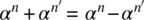 . Also show that
  for
for  .
.
REFERENCES
- 1. C. Berrou, A. Glavieux, P. Thitimajshima, “Near Shannon Limit Error‐Correcting Coding and Decoding: Turbo Codes,” IEEE Proceedings of ICC ’93, pp. 1064–1070, Geneva, Switzerland, May 1993. (This paper is reprinted in IEEE Transactions on Communications, October 1996—see Reference 107).
- 2. M.R. Aaron, “PCM Transmission in the Exchange Plant,” The Bell System Technical Journal, Vol. 41, No. 1, pp. 99–141, January 1962.
- 3. Inter‐Range Instrumentation Group (IRIG) Telemetry Standard, Range Commanders Council (RCC) Document, 106–05.
- 4. H.L. Deffebach, W.O. Frost, “A Survey of Digital Baseband Signaling Techniques,” NASA Technical Memorandum X‐64615, George C. Marshall Space Flight Center, Alabama, June 30, 1971.
- 5. W. Stallings, “Digital Signaling Techniques,” IEEE Communications Magazine, Vol. 22, No. 12, pp. 21–25, December 1984.
- 6. W.R. Bennett, “Statistics of Regenerative Digital Transmission,” Bell System Technical Journal, Vol. 37, No. 6, pp. 1501–1542, November 1958.
- 7. R.C. Titsworth, L.R. Welch, “Power Spectra of Signals Modulated by Random and Pseudorandom Sequences,” Technical Report 32–140, Jet Propulsion Laboratory, Pasadena, CA, October 1961.
- 8. W.C. Lindsey, M.K. Simon, Telecommunication Systems Engineering, Dover Publications, Inc., New York, 1773.
- 9. R.C. Houts, T.A. Green, “Comparing Bandwidth Requirements for Binary Baseband Signals,” IEEE Transactions on Communications, Vol. COM‐12, No. 6, pp. 776–781, June 1973.
- 10. E.D. Sunde, “Theoretical Fundamentals of Pulse Transmission,” Bell System Technical Journal, Part I, Vol. 33, pp. 721–788, May 1954 and Part II, Vol. 33, pp. 25–97, July 1954.
- 11. V. Johannes, A. Kaim, T. Walzman, “Bipolar Pulse Transmission with Zero Extraction,” IEEE Transactions on Communication Technology, Vol. COM‐17, No. 2, pp. 303–310, April 1969.
- 12. K.E. Fultz, D.B. Penick, “The T1 Carrier System,” Bell System Technical Journal, Vol. 44, No. 7, pp. 1405–1451, September 1965.
- 13. B.H. Batson, “An Analysis of the Relative Merits of Various PCM Code Formats,” Report MSC‐EB‐R‐68‐5, NASA Manned Spacecraft Center, Houston, TX, 1 November 1968.
- 14. M. Hecht, A. Guida, “Delay Modulation,” Proceeding of the IEEE, Vol. 57, No. 7, pp. 1314–1316, July 1969.
- 15. Range Commanders Council (RCC), Telemetry Applications Handbook, RCC‐119‐06, May 2006.
- 16. W.N. Waggener, Pulse Code Modulation Systems Design, Artech House, Boston, MA, 1998.
- 17. R.M. Gagliardi, Introduction to Communications Engineering, John Wiley & Sons, Inc., New York 1978.
- 18. I. Korn, “Error Probability and Bandwidth of Digital Modulation,” IEEE Transactions on Communications, Vol. COM‐28 No. 2, pp. 287–290, February 1980.
- 19. E.L. Law, “Optimized Low Bit Rate PCM/FM Telemetry with Wide IF Bandwidths,” Proceedings of the International Telemetering Conference, San Diego, CA, October 2002.
- 20. Range Commanders Council (RCC), Telemetry Applications Handbook, RCC‐119‐06, May 2006, Chapter 2, Sections 2.1.1, 2.1.2, and 2.2.
- 21. C.H. Tan, T.T. Tjhung, H. Singh, “Performance of Narrow‐Band Manchester Coded FSK with Discriminator Detection,” IEEE Transactions on Communications, Vol. COM‐31, No. 5, pp. 659–667, May 1983.
- 22. D.E. Cartier, “Limiter‐Discriminator Detection Performance of Manchester and NRZ Coded FSK,” IEEE Transactions on Aerospace and Electronic Systems, Vol. AES‐13, No. 1, pp. 62–70, January 1977.
- 23. W.P. Osborne, M.B. Luntz, “Coherent and Noncoherent Detection of CPFSK”, IEEE Transactions on Communications, Vol. COM‐22, No. 8, pp. 1023–1036, August 1974.
- 24. M.S. Geoghegan, “Improving the Detection Efficiency of Conventional PCM/FM Telemetry by using a Multi‐Symbol Demodulator,” Proceedings of the 2000 International Telemetering Conference, Volume XXXVI, pp. 717–724, San Diego, CA, October 2000.
- 25. Range Commanders Council (RCC), Telemetry Applications Handbook, RCC‐119‐06, May 2006, Chapter 2, Section 2.2.8.
- 26. E. L. Law, K. Feher, “FQPSK versus PCM/FM for Aeronautical Telemetry Applications: Spectral Occupancy and Bit‐error Probability Comparisons,” Proceedings of the International Telemetering Conference, Las Vegas, NV, October 1997.
- 27. M.G. Pelchat, “The Autocorrelation Function and Power Spectrum of PCM/FM with Random Binary Modulating Waveforms,” IEEE Transactions on Space Electronics and Telemetry, Vol. SET‐10, No. 1, pp. 39–44, March 1964.
- 28. E.L. Law, “RF Spectral Characteristics of Random PCM/FM and PSK Signals,” Proceedings of the International Telemetering Conference, Los Vegas, NV, November 4–7, 1991.
- 29. A.D. Watt, V.J. Zurick, R.M. Coon, “Reduction of Adjacent‐Channel Interference Components from Frequency‐Shift‐Keyed Carriers,” IRE Transactions on Communication Systems, Vol. CS‐6, No. 12, pp. 39–47, December 1958.
- 30. S. W. Golomb, “Sequence with Randomness Properties,” Glen L. Martin Company, Internal Report, Baltimore, MD, June 14, 1955.
- 31. R. Gold, “Properties of Linear Binary Encoding Sequences,” Lecture Notes, Robert Gold Associates, Los Angeles, CA, July 1975.
- 32. W.W. Peterson, E.J. Weldon, Jr., Error‐Correcting Codes, Second Edition, The MIT Press, Cambridge, MA, 1972, Chapter 7.
- 33. W.W. Peterson, E.J. Weldon, Jr., Error‐Correcting Codes, Second Edition, The MIT Press, Cambridge, MA, 1972, Chapter 6.
- 34. W.W. Peterson, E.J. Weldon, Jr., Error‐Correcting Codes, Second Edition, The MIT Press, Cambridge, MA, 1972.
- 35. M.P. Ristenbatt, “Pseudo Binary Coded Waveforms,” R.S. Berkowitz, Editor, Modern Radar, Analysis, Evaluation and System Design, p. 296, Part IV, Chapter 4, John Wiley & Sons, Inc., New York, 1966.
- 36. R. Gold, “Properties of Linear Binary Encoding Sequences,” Lecture Notes, Robert Gold Associates, Los Angeles, CA, July 1975, p. 6–2.
- 37. S. Lin, An Introduction to Error‐Correcting Codes, Prentice‐Hall, Inc., Englewood Cliffs, NJ, 1970. (This reference includes a discussion of burst‐error correcting codes.)
- 38. W.W. Peterson, E.J. Weldon, Jr., Error‐Correcting Codes, Second Edition, The MIT Press, Cambridge, MA, 1972, Appendix C.
- 39. S. Lin, An Introduction to Error‐Correcting Codes, pp. 58–70, Prentice‐Hall, Inc., Englewood Cliffs, NJ, 1970.
- 40. F.J. MacWilliams, “A Theorem on the Distribution of Weights in Systematic Code,” Bell System Technical Journal, Vol. 42, pp. 79–94, 1963.
- 41. W.W. Peterson, E.J. Weldon, Jr., Error‐Correcting Codes, Second Edition, The MIT Press, Cambridge, MA, 1972, pp. 64–70.
- 42. J.L. Massey, “Coding Techniques for Digital Data Networks,” Proceedings of the International Conference on Information Theory and Systems,” NTG‐Fachberichte, Vol. 65, pp. 18–20, Berlin, Germany, September 1978.
- 43. T. Fujiwara, T. Kasami, A. Kitai, S. Lin, “On the Undetected Error Probability for Shortened Hamming Codes,” IEEE Transactions on Communications, Vol. COM‐33, No. 6, pp. 570–574, June 1985.
- 44. J.K. Wolf, R.D. Blakeney, II, “An Exact Evaluation of the Probability of Undetected Error for Certain Shortened Binary CRC Codes,” IEEE Military Communications Conference, MILCOM ’88, Vol. 1, pp. 0287–0292, San Diego, CA, October 23–26, 1988.
- 45. M. Abramowitz, I.A. Stegun, Editors, Handbook of Mathematical Functions with Formulas, Graphs, and Mathematical Tables, National Bureau of Standards, Applied Mathematics Series No. 55, pp. 949–950, November 1964.
- 46. F. Jager, C.B. Dekker, “Tamed Frequency Modulation, A Novel Method to Achieve Spectrum Economy in Digital Transmission,” IEEE Transactions on Communications, Vol. COM‐26, No. 5, pp. 534–542, May 1978.
- 47. D. Muilwijk, “Tamed Frequency Modulation—A Bandwidth‐Saving Digital Modulation Method, Suited for Mobile Radio,” Philips Telecommunication Review, Vol. 37, No. 3, pp. 35–49, March 1979.
- 48. S. Bellini, M. Sonzogni, G. Tartara, “Noncoherent Detection of Tamed Frequency Modulation,” IEEE Transactions on Communications, Vol. COM‐32, No. 3, pp. 218–224, March 1984.
- 49. K. Chung, “Generalized Tamed Frequency Modulation and Its Application for Mobile Radio Communications,” IEEE Transactions on Selected Areas in Communications, Vol. SAC‐2, No. 4, pp. 487–497, July 1984.
- 50. J.L. Ramsey, “Realization of Optimum Interleavers,” IEEE Transactions on Information Theory, Vol. IT‐16, No. 3, pp. 338–345, May 1970.
- 51. G.D. Forney, Jr., “Burst‐Correcting Codes for the Classic Bursty Channel,” IEEE Transactions on Communication Technology, Vol. COM‐19, pp. 772–781, October, 1971.
- 52. D.D. Newman, “Observations of the Nature and Effects of Interleavers in Communications Links,” Final Report AFWL‐TR‐82‐125, Air Force Weapons Laboratory, Kirtland Air Force Base, NM, February 1983.
- 53. A. Papoulis, Probability, Random Variables and Stochastic Processes pp. 57–63, McGraw‐Hill, New York, 1965.
- 54. J.M. Wozencraft, “Sequential Decoding for Reliable Communications,” Technical Report 325, Research Laboratories of Electronics, The MIT Press, Cambridge, MA, 1957.
- 55. R.M. Fano, “A Heuristic Discussion of Probabilistic Decoding,” IEEE Transactions on Information Theory, Vol. IT‐9, pp. 64–74, 1963.
- 56. J.L. Massey, D.J. Costello, Jr., “Nonsystematic Convolutional Codes for Sequential Decoding in Space Applications,” IEEE Transactions on Communication Technology, Part II, Vol. COM‐19, pp. 806–813, October, 1971.
- 57. J.A. Heller, I. M. Jacobs, “Viterbi Decoding for Satellite and Space Communications,” IEEE Transactions on Communication Technology, Vol. COM‐19, No. 5, pp. 835–848, October 1971.
- 58. W.W. Peterson, Error‐Correcting Codes, The MIT Press, Cambridge, MA, 1961.
- 59. A.J. Viterbi, Principles of Coherent Communications, McGraw‐Hill, New York, 1966.
- 60. S. Lin, An Introduction to Error‐Correcting Codes, Chapters 10–13, Prentice‐Hall, Inc., Englewood Cliffs, NJ, 1970.
- 61. W. W. Peterson, E. J. Weldon, Jr., Error‐Correcting Codes, Chapters 13 and 14, The MIT Press, Cambridge, MA, 1972.
- 62. A.J. Viterbi, J.K. Omura, Principles of Digital Communication and Coding, McGraw‐Hill, New York, 1966.
- 63. A.M. Michelson, A.H. Levesque, Error‐Control Techniques for Digital Communication, John Wiley & Sons, Inc., New York, 1985.
- 64. J.P. Odenwalder, “Error Control Coding Handbook,” United Sates Air Force, Contract No. F44620‐76‐C‐0056, Final Report, Linkabit Corporation, July 15, 1976.
- 65. S. Benedetto, D. Divsalar, “Turbo Codes: Principles and Applications,” Coarse Notes Presented at Titan Linkabit, July 28–30, 1997.
- 66. S. Benedetto, G. Montorsi, “Bandwidth Efficient, Versatile Concatenated Coded Schemes with Interleavers,” Presented at Titan Linkabit, July 29, 1999.
- 67. Y. Yasuda, K. Kashiki, Y. Hirata, “High‐Rate Punctured Convolutional Codes for Soft Decision Viterbi Decoding,” IEEE Transactions on Communications, Vol. COM‐32, No. 3, pp. 315–319, March 1984.
- 68. A.J. Viterbi, “Error Bounds for Convolutional Codes and an Asymptotically Optimum Decoding Algorithm,” IEEE Transactions on Information Theory, Vol. IT‐13, pp. 260–269, 1967.
- 69. G.D. Forney, Jr., “The Viterbi Algorithm,” Proceedings of the IEEE, Vol. 61, No. 3, pp. 268–278, March 1973.
- 70. G.D. Forney, Jr., “Convolutional Codes II: Maximum Likelihood Decoding,” Technical Report 7004–1, Stanford Electronics Laboratories, Stanford, CA, June 1972.
- 71. G.D. Forney, Jr., “Coding and Its Application in Space Communications,” IEEE Spectrum, June 1970.
- 72. J.A. Heller, “Short Constraint Length Convolutional Codes,” Space Programs Summary 37–54, Vol. III, pp. 171–177, Jet Propulsion Laboratory, California Institute of Technology, October/November, 1968.
- 73. J.A. Heller, “Improved Performance of Short Constraint Length Convolutional Codes,” Space Programs Summary 37–56, Vol. III, pp. 83–84, Jet Propulsion Laboratory, California Institute of Technology, February/March 1969.
- 74. C.M. Rader, “Memory Management in a Viterbi Decoder,” IEEE Transactions on Communications, Vol. COM‐29, No. 9, pp. 1399–1401, September, 1981.
- 75. J.L. Massey, “Catastrophic Error‐Propagation in Convolutional Codes,” Proceedings, Eleventh Midwest Symposium on Circuit Theory, University of Notre Dame, Notre Dame, Indiana, May 13–14, 1968.
- 76. J.P. Odenwalder, “Optimum Decoding of Convolutional Codes,” Ph.D. dissertation, University of California, Los Angeles, CA, 1970.
- 77. E. Paaske, “Short Binary Convolutional Codes with Maximal Free Distance for Rates 2/3 and 3/4,” IEEE Transactions on Information Theory, Vol. IT‐20, pp. 683–689, September 1974.
- 78. A. M. Michelson, A. H. Levesque, Error‐Control Techniques for Digital Communication, John Wiley & Sons, Inc., New York, 1985, Section 9.5.4.
- 79. K.J. Larsen, “Short Convolutional Codes with Maximal Free Distance for Rates 1/2, 1/3, and 1/4,” IEEE Transactions on Information Theory, IT‐19, pp. 371–372, May 1973.
- 80. R.L. Peterson, R.E. Ziemer, D.E. Borth, Introduction to Spread Spectrum Communications, Chapter 9, Section 4.1, Prentice Hall, Englewood Cliffs, NJ, 1995.
- 81. D.G. Daut, J.W. Modestino, L.D. Wismer, “New Short Constraint Length Convolutional Code Construction for Selected Rational Rates,” IEEE Transactions on Information Theory, Vol. IT‐28, pp. 793–799, September 1982.
- 82. B.D. Trumpis, “Convolutional Coding for M‐ary Channels,” Ph.D. dissertation, University of California, Los Angeles, CA, 1975.
- 83. G.D. Forney, Jr., “Structural Analysis of Convolutional Codes via Dual Codes,” IEEE Transactions on Information Theory, Vol. IT‐19, pp. 512–518, July, 1973.
- 84. G.D. Forney, Jr., “Convolutional Codes I: Algebraic Structure,” IEEE Transactions on Information Theory, Vol. IT‐16, pp. 720–738, November 1970.
- 85. J. G. Proakis, Digital Communications, Second Edition, pp. 468–473, McGraw‐Hill, New York, 1989.
- 86. A.J. Viterbi, I.M. Jacobs, “Advances in Coding and Modulation for Noncoherent Channels Affected by Fading, Partial Band, and Multiple‐Access Interference,” A.J. Viterbi, Editor, Advances in Communication Systems, Vol. 4, Academic Press, New York, 1975.
- 87. J.G. Proakis, I. Rahman, “Performance of Concatenated Dual‐k Codes on a Rayleigh Fading Channel with a Bandwidth Constraint,” IEEE Transactions on Communications, Vol. COM‐27, No. 5, pp. 801–806, May 1979.
- 88. A.J. Viterbi, “Convolutional Codes and Their Performance in Communication Systems,” IEEE Transactions on Communication Technology, Vol. COM‐19, No. 5, pp. 751–772, October 1971.
- 89. A.J. Viterbi, “The State‐Diagram Approach to Optimal Decoding and Performance Analysis for Memoryless Channels,” Space Programs Summary, 37–38, Vol. III, pp. 50–55, Jet Propulsion Laboratory, 1969.
- 90. J.P. Odenwalder, “Dual‐k Convolutional Codes for Noncoherently Demodulated Channels,” Proceeding of the International Telemetering Conference, Vol. 12, pp. 165–174, September 1976.
- 91. J.B. Cain, G.C. Clark, Jr., J.M. Geist, “Punctured Convolutional Codes of Rate (n‐1)/n and Simplified Maximum Likelihood Decoding,” IEEE Transactions on Information Theory, Vol. IT‐25, No. 1, pp. 97–100, January 1979.
- 92. J.K. Wolf, E. Zehavi, “P2 Codes: Pragmatic Trellis Codes Utilizing Punctured Convolutional Codes,” IEEE Communications Magazine, Vol. 33, No. 2, pp. 94–99, February 1995.
- 93. A.J. Viterbi, J.K. Wolf, E. Zehavi, R. Padovani, “A Pragmatic Approach to Trellis‐Coded Modulation,” IEEE Communications Magazine, Vol. 27, No. 7, pp. 11–19, July, 1989.
- 94. G. Ungerboeck, “Channel Coding with Multilevel/Phase Signals,” IEEE Transactions on Information Theory, Vol. IT‐28, pp. 55–67, January 1982.
- 95. Qualcomm, Q1900 Viterbi/Trellis Decoder, Qualcomm Corporation, ASIC Products, San Diego, CA, 1991.
- 96. G.D. Forney, Jr., Concatenated Codes, The MIT Press, Cambridge, MA, 1966.
- 97. J. P. Odenwalder, “Optimum Decoding of Convolutional Codes,” Ph.D. dissertation, University of California, Los Angeles, CA, 1970, Chapter 6.
- 98. J.P. Odenwalder, “Error Control Coding Handbook,” United Sates Air Force, Contract No. F44620‐76‐C‐0056, Final Report, Linkabit Corporation, July 15, 1976, Section 6.0, pp. 183–189.
- 99. J.M. Wozencraft, I.M. Jacobs, Principles of Communication Engineering, Chapter 7, John Wiley & Sons, Inc., New York, 1967.
- 100. S. Benedetto, D. Divsalar, G. Montorsi, F. Pollara, “Parallel Concatenated Trellis Coded Modulation,” IEEE Proceedings of ICC’96, San Diego, CA, October 28–31, 1996.
- 101. D. Divsalar, F. Pollara, “Turbo Codes for PCS Applications,” Proceedings of IEEE Proceedings of ICC’95, Seattle, Washington, June 1995.
- 102. C. Heegard, S.B. Wicker, Turbo Coding, Kluwer Academic Publishers, Boston, MA, 1999.
- 103. S. Benedetto, D. Divsalar, G. Montorsi, F. Pollara, “Serial Concatenation of Interleaved Codes: Performance Analysis, Design, and Iterative Decoding,” The JPL TDA Progress Report 42–126, August 15, 1996.
- 104. S. Benedetto, D. Divsalar, G. Montorsi, F. Pollara, “Soft‐Out Decoding Algorithms in Iterative Decoding of Turbo Codes,” TDA Progress Report 42–124, JPL, CalTech, Pasadena, CA, February 15, 1996. Also appears in IEEE Proceedings of ICC’96, Dallas, TX, pp. 112–117, June 1996.
- 105. D. Divsalar, “Iterative Decoding of Turbo, Serial, Hybrid, and Self Concatenated Codes,” JPL‐CALTECH, October, 1998. (Provides performance summaries for: PCCC, p. 71; SCCC p.845‐86; DPCCC, p. 94, 95; HCCC, p. 114, 115; Self Concatenated Code, p. 123.)
- 106. D. Divsalar, R.J. McEliece, The Effective Free Distance of Turbo Codes, Jet Propulsion Laboratory, California Institute of Technology, Pasadena, CA, December 1995.
- 107. B. Vucetic, Y. Li, L.C. Perez, F. Jiang, “Recent Advances in Turbo Code Design and Theory,” Proceedings of the IEEE, Vol. 95, No. 6, pp. 1323–1344, June 2007.
- 108. J.D. Anderson, V.V. Zybolv, “Interleaver Design for Turbo Coding,” International Symposium on Turbo Codes, Brest, France, 1997.
- 109. J. Yuan, S.G. Wilson, “Multiple Output Sliding Window Decoding Algorithm for Turbo Codes,” Proceeding of CISS’97, Baltimore, MD, March 1997.
- 110. C. Berrou, A. Glavieux, “Near Optimum Error Correcting Coding and Decoding: Turbo‐Codes,” IEEE Transactions on Communications, Vol. 44, No. 10, pp. 1261–1271, October 1996. (This paper was presented at ICC’93, Geneva, Switzerland, May 1993).
- 111. D. Divsalar, F. Pollara, “Multiple Turbo Codes for Deep‐Space Communications,” JPL TDA Progress Report 42–121, Jet Propulsion Laboratory, Pasadena, CA, May 1995.
- 112. S. Dolinar, D. Divsalar, F. Pollara, “Code Performance as a Function of Block Size,” TMO Progress Report 42–133, JPL, May 1998.
- 113. S.W. Golomb, H. Taylor, “Constructions and Properties of Costas Arrays,” Proceedings of the IEEE, Vol. 72, No. 9, pp. 1143–1163, September 1984.
- 114. S.B. Wicker, Error Control Systems for Digital Communications and Storage, Prentice Hall, Englewood Cliffs, NJ, 1995.
- 115. S. Benedetto, G. Montorsi, D. Divsalar, F. Pollara, “A Soft‐In Soft‐Out Maximum A Posteriori (MAP) Module to Decode Parallel and Serial Concatenated Codes,” TDA Progress Report 42–127, November 15, 1996.
- 116. S. Benedetto, G. Montorsi, “Unveiling Turbo Codes: Some Results on Parallel Concatenated Coding Schemes,” IEEE Transactions on Information Theory, Vol. 42, No. 2, pp. 409–429, March 1966.
- 117. D. Divsalar, “Iterative Decoding of Turbo, Serial, Hybrid, and Self Concatenated Codes,” JPL‐CALTECH, October 1998. (Provides equations for forward and backward recursion processing within the SISO module).
- 118. D. Divsalar, “Iterative Decoding of Turbo, Serial, Hybrid, and Self Concatenated Codes,” JPL‐CALTECH, October, 1998. Presents the algorithms for the SCCC two‐SISO inner code recursions, pp. 78, 79, outer code recursions, and output bit reliability, pp. 80–82.
- 119. S. Benedetto, D. Divsalar, G. Montorsi, F Pollara, “Analysis, Design, and Iterative Decoding of Double Serially Concatenated Codes with Interleaves,” IEEE Transactions on Selected Areas in Communications, Vol. 16, No. 2, pp. 231–244, February 1998.
- 120. S. Benedetto, D. Divsalar, G. Montorsi, F. Pollara, “A Soft‐Input Soft‐Output AAP Module for Iterative Decoding of Concatenated Codes,” Interim Report, Partially supported by NATO Grant RG951208, partially carried out at JPL CALTECH under contract with NASA, January 3, 1997.
- 121. S. Benedetto, D. Divsalar, G. Montorsi, “Turbo‐Like Codes Constructions,” Chapter 2, D. Declercq, M. Fossorier, E. Biglieri, Editors, Channel Coding Theory, Algorithms, and Applications, pp. 53–140, Academic Press Library in Mobile and Wireless Communications, Elsevier Books, Oxford, 2014.
- 122. L.R. Bahl, J. Cocke, F. Jelinek, J. Raviv, “Optimal Decoding of Linear Codes for Minimizing Symbol Error Rate,” IEEE Transactions on Information Theory, Vol. IT‐20, pp. 284–287, March 1974.
- 123. D. Divsalar, “Iterative Decoding of Turbo, Serial, Hybrid, and Self Concatenated Codes,” p. 41, JPL‐CALTECH, October 1998.
- 124. Y. Wu, B.D. Woerner, T.K. Blankenship, “Data Width Requirements in SISO Decoding with Modulo Normalization,” IEEE Transactions on Communications, Vol. 49, No. 11, pp. 1861–1868, November 2001.
- 125. Consultative Committee for Space Data Systems (CCSDS), Blue Book, CCSDS 101.0‐B‐6, Section 4, Turbo Coding, October 2002.
- 126. Consultative Committee for Space Data Systems (CCSDS), Recommendation for Space Data System Standards, “Telemetry Channel Coding,” CCSDS 101.0‐B‐6, Blue Book, pp. 4–5, October 2002.
- 127. C. Douillard, M. Jezequel, “Turbo Codes: From First Principles to Recent Standards,” Chapter 1, D. Declercq, M. Fossorier, E. Biglieri, Editors, Channel Coding Theory, Algorithms, and Applications, pp. 1–52, Academic Press Library in Mobile and Wireless Communications, Elsevier Books, Oxford, 2014.
- 128. S. Dolinar, D. Divsalar, F. Pollara, “Code Performance as a Function of Block Size,” JPL TDA Progress Report 42–130, Jet Propulsion Laboratory, Pasadena, CA, August 1998.
- 129. S. Dolinar, D. Divsalar, F. Pollara, “Turbo Codes and Space Communications,” Communications Systems and Research Section, Jet Propulsion Laboratory, CalTech, Pasadena, CA, 1998.
- 130. S. Benedetto, G. Montorsi, “Design of Parallel Concatenated Convolutional Codes,” IEEE Transactions on Communications, Vol. 44, No. 5, pp. 591–600, May 1996.
- 131. R.G. Gallager, “Low‐Density Parity‐Check Codes,” Institute of Radio Engineers, Vol. IT‐8, pp. 21–28, January 1962. Also, reprinted in the “The Development of Coding Theory,” Editor E.R. Berlekamp, IEEE Press, Part II: Constructions for Block Codes, pp. 121–128, New York, 1974.
- 132. D.J.C. MacKay, “Good Error‐Correcting Codes Based on Very Sparse Matrices,” IEEE Transactions on Information Theory, Vol. 45, No. 3, pp. 399–431, March 1999.
- 133. D.J. Costello, Jr., G.D. Forney, Jr., “Channel Coding: The Road to Channel Capacity,” Proceedings of the IEEE, Vol. 95, No. 6, pp. 1150–1177, June 2007.
- 134. D. Slepian, “A Class of Binary Signaling Alphabets,” Bell System Technical Journal, Vol. 35, pp. 203–234, January 1956.
- 135. D. Sridhara, T. Fuja, R.M. Tanner, “Low Density Parity‐Check Codes form Permutation Matrices,” Conference on Information Sciences and Systems, The John Hopkins University, March 2001.
- 136. M. Luby, M. Mitzenmacher, M.A. Shokrollahi, D.A. Spielman, “Improved Low‐Density Parity‐Check Codes using Irregular Graphs,” IEEE Transactions on Information Theory, Vol. 47, No. 2, pp. 585–598, February 2001.
- 137. T.J. Richardson, M.A. Shokrollahi, R.L. Urbanke, “Design of Capacity‐Approaching Irregular Low‐Density Parity‐Check Codes,” IEEE Transactions on Information Theory, Vol. 47, No. 2, pp. 619–637, February 2001.
- 138. R.G. Gallager, “Low‐Density Parity‐Check Codes,” Sc. D. thesis, Massachusetts Institute of Technology, Cambridge, MA, September 1960.
- 139. R.G. Gallager, “Low‐Density Parity‐Check Codes,” Institute of Radio Engineers, Vol. IT‐8, pp. 21–28, January 1962. Also, reprinted in the “The Development of Coding Theory”, Editor E.R. Berlekamp, IEEE Press, Part II: Constructions for Block Codes, page 122, Table 3, New York, 1974.
- 140. K. Gracie, M.H. Hamon, “Turbo and Turbo‐Like Codes: Principles and Applications in Telecommunications,” Proceedings of the IEEE, Vol. 95, No. 6, pp. 1228–1254, June 2007.
- 141. C.‐H. Liu, S.‐W. Yen, C.‐L. Chen, H.‐C. Chang, C.‐Y. Lee, Y.‐S. Hsu, S.‐J. Jou, “An LDPC Decoder Based on Self‐Routing Network for IEEE 802.16e Applications,” IEEE Journal on Solid‐State Circuits, Vol. 43, No. 3, pp. 684–694, March 2008.
- 142. K. Gracie, M.H. Hamon, “Turbo and Turbo‐Like Codes: Principles and Applications in Telecommunications,” Proceedings of the IEEE, Vol. 95, No. 6, p. 1235, Figure 9 and p. 1236, Figure 12, June 2007.
- 143. D. Williams, “Turbo‐Charging Next‐Gen Wireless, Optical Systems,” Communication Systems Design, Vol. 7, No. 2, pp. 39–47, February 2001.
- 144. R. Pyndiah, A. Glavieux, A. Picart, S. Jacq, “Near Optimum Decoding of Product Codes,” Proceeding of Global Telecommunications Conference (Globecom’94), pp. 339–343, San Francisco, CA, November 28–December 2, 1994.
- 145. R.M. Pyndiah, “Near‐Optimum Decoding of Product Codes: Block Turbo Codes,” IEEE Transactions on Communications, Vol. 46, No. 8, pp. 1003–1010, August 1998.
- 146. K. Gracie, M.H. Hamon, “Turbo and Turbo‐Like Codes: Principles and Applications in Telecommunications,” Proceedings of the IEEE, Vol. 95, No. 6, pp. 1233–1234, June 2007.
- 147. J. Fang, F. Buda, E. Lemois, “Turbo Product Codes: A Well Suitable Solution to Wireless Packet Transmissions for Very Low Error Rates,” Proceedings of the 2nd International Symposium on Turbo Codes and Related Topics,” pp. 101–111, Brest, France, September 2000.
- 148. S.Y. Chung, G.D. Forney, Jr., T.J. Richardson, R. Urbanke, “On the Design of Low‐Density Parity‐Check Codes Within 0.0045 dB from the Shannon Limit,” IEEE Communication Letters, Vol. 5, No. 2, pp. 58–60, February 2001.
- 149. C. Berrou, J. Hagenauer, M. Luise, C. Schlegel, and L. Vandendorpe, Editors, “Turbo‐Information Processing: Algorithms, Implementations, and Applications,” Special Issue, Proceeding of the IEEE,” Vol. 95, No. 6, June 2007.
- 150. W.W. Peterson, E.J. Weldon, Jr., Error‐Correction Codes, Second Edition, Chapter 12, The MIT Press, Cambridge, MA, 1972.
- 151. C. Herzet, N. Noels, V. Lottici, H. Wymeersch, M. Luise, M. Moeneclaey, L. Vandendorpe, “Code‐Aided Turbo Synchronization,” Proceeding of the IEEE, Vol. 95, No. 6, pp. 1255–1271, June 2007.
- 152. Consultative Committee for Space Data Systems (CCSDS), Blue Book, CCSDS 101.0‐B‐6, October 2002. Turbo Code Synchronization, Section 4, Specification 10; Frame Synchronization, Section 5.
- 153. A. Anastasopoulos, K.M. Chugg, G. Colavolpe, G. Ferrari, R. Raheli, “Interactive Detection for Channels with Memory,” Proceedings of the IEEE, Vol. 95, No. 6, pp. 1272–1294, June 2007.
- 154. W.W. Peterson, E.J. Weldon, Jr., Error‐Correcting Codes, Second Edition, pp. 274 and 275, The MIT Press, Cambridge, MA, 1972, Chapter 9.
- 155. W.W. Peterson, E.J. Weldon, Jr., Error‐Correcting Codes, Second Edition, pp. 493–534, The MIT Press, Cambridge, MA, 1972, Appendix D.
- 156. C.L. Chen, “Some Results on Algebraically Structured Error‐Correction Codes,” Ph.D. dissertation, University of Hawaii, 1969.
- 157. M.J. Weiss, R. Dubisch, Higher Algebra for the Undergraduate, John Wiley & Sons, Inc., New York, 1962.
- 158. R.W. Marsh, Table of Irreducible Polynomials over GF(2) Through Degree 19, NSA, Washington, DC, 1957.
- 159. S. Lin, An Introduction to Error‐Correcting Codes, pp. 21–23; 112–119, Prentice‐Hall, Inc., Englewood Cliffs, NJ, 1970
- 160. S. Lin, D.J. Costello, Jr., Error Control Coding: Fundamentals and Applications, Prentice‐Hall, Inc., Englewood Cliffs, NJ, 1983.
- 161. J.P. Stenbit, “Table of Generators for Bose‐Chaudhuri Codes,” IEEE Transactions on Information Theory, Vol. IT‐10, pp. 390–391, January 1964.
- 162. J.L. Massey, “Shift‐Register Synthesis and BCH Decoding,” IEEE Transactions on Information Theory, Vol. IT‐15, pp. 122–127, January 1969.
- 163. W.W. Peterson, E.J. Weldon, Jr., Error‐Correcting Codes, Second Edition, The MIT Press, Cambridge, MA, 1972, pp. 289–296.
- 164. E.R. Berlekamp, “On Decoding Binary Bose‐Chaudhuri‐Hocquenghem Codes,” IEEE Transactions on Information Theory, Vol. IT‐11, pp. 577–580, October 1965.
- 165. G.D. Forney, Jr., “On Decoding BCH Codes,” IEEE Transactions on Information Theory, Vol. IT‐11, pp. 549–557, October 1965.
- 166. S. Lin, An Introduction to Error‐Correcting Codes, Prentice‐Hall, Inc., Englewood Cliffs, NJ, 1970, pp. 122, 125.
- 167. E.R. Berlekamp, Algebraic Coding Theory, McGraw‐Hill, New York, 1968.