
20
IONOSPHERIC PROPAGATION
20.1 INTRODUCTION
The amplitude variations of a signal propagating through the ionosphere [1] result from the destructive and constructive interaction of the signal phase resulting from the numerous signal paths through the nonhomogeneous medium; this phenomenon is referred to as scintillation. In addition to scintillation, signal propagation through the ionosphere is subjected to anomalies characterized by time delay variations, angular errors caused by refractive bending, frequency shifts, dispersion, polarization rotation, and absorption that must be accounted for in the communication link budget. Refractive bending affects azimuth and elevation measurement accuracies while time delay and frequency variations result in range and velocity estimation errors. Dispersion gives rise to symbol broadening and intersymbol interference (ISI) that degrade the symbol‐error performance while polarization rotation and absorption can significantly degrade the available link margin. These errors also impact antenna, symbol, and carrier tracking loops contributing to degraded communication performance.
Signal propagation through the ionosphere is characterized by the refractive index. The refractive index and its influence on the various aspects of a received signal is the subject of this chapter. The significant parameters that influence the signal propagation through the ionosphere are the electron density ![]() with units of electrons per cubic‐centimeter and the total electron content (TEC or NT) along the propagation path of length ℓ. The electron density is generally specified in terms of electrons/cubic‐centimeter; however, the following analysis uses the mks system of units with the TEC specified in terms of electrons/square‐meter. The TEC is computed as
with units of electrons per cubic‐centimeter and the total electron content (TEC or NT) along the propagation path of length ℓ. The electron density is generally specified in terms of electrons/cubic‐centimeter; however, the following analysis uses the mks system of units with the TEC specified in terms of electrons/square‐meter. The TEC is computed as

where ![]() electrons/m3.
electrons/m3.
In Sections 20.2 and 20.3 the electron densities in the ionosphere are characterized for the natural and nuclear‐disturbed environments and the influence of the electron densities on signal propagation is discussed in Section 20.4 in terms of the refractive index. With this background material the electron density is used to characterize signal scintillation in Section 20.5 in terms of the signal decorrelation time τo, frequency‐selective bandwidth fo, dispersion, and absorption. Although the focus in this section is on the nuclear environment, the results are also applicable to electron densities occurring naturally. In Section 20.6 the Rayleigh fading channel is described and the results are used to outline the development of a computer simulation program for simulating the performance of a communication link with various waveform modulations, forward error correction (FEC) coding, combining, and interleaving techniques. The chapter concludes with a case study of a scintillation scenario using a differentially coherent modulation with interleaving and combining.
20.2 ELECTRON DENSITIES: NATURAL ENVIRONMENT
The electron density content of the natural ionosphere has been modeled by Chapman [2] as1
where h is the vertical height above the Earth’s surface, ![]() is the maximum electron density where hm is the height of maximum electron density, θ is the solar zenith angle, and Z is a normalized height parameter expressed as
is the maximum electron density where hm is the height of maximum electron density, θ is the solar zenith angle, and Z is a normalized height parameter expressed as
where H is a scale height given by
Using the mks system of units, k = 1.372 × 10⁻²³ J/°K is Boltzmann’s constant, T is temperature in degrees Kelvin, ma is the mean mass of an air molecule, and g = 9.7538 m/s2 is the gravitational acceleration at the Earth’s surface. The product mag = 4.8 × 10⁻²⁶ kg is the mean weight of an air molecule and the factor 0.10197 converts joules to kilogram‐meters. Using these parameters the scale height H given by (20.4) is in meters at the Earth’s surface and, upon conversion to kilometers, is evaluated as ![]() km or 8.452 km when T = 290°K. However, the parameters ma, g, and T are functions of height and Davies [3] provides an approximation to (20.4) at a height h given by
km or 8.452 km when T = 290°K. However, the parameters ma, g, and T are functions of height and Davies [3] provides an approximation to (20.4) at a height h given by

where h is in kilometers, Re ≅ 6370 km is the Earth’s radius, and M is the molecular weight in grams/mole. The dependence of the parameters T and M on h is tabulated in Table 20.1 for the 1959 Air Research and Development Command (ARDC) model atmosphere [4]. The 1959 ARDC model atmosphere is a revision of the 1956 model atmosphere that includes new rocket and satellite data; the data up to 53 km is the same in each model. Additional details and various assumptions are also provided by Davies [3].
TABLE 20.1 Dependence of the Parameters T and M on Height ha
| h (km) | T (K) | M (g/mol) |
| 0 | 288 | 28.966 |
| 10 | 223 | 28.966 |
| 20 | 217 | 28.966 |
| 30 | 231 | 28.966 |
| 40 | 261 | 28.966 |
| 50 | 283 | 28.966 |
| 60 | 254 | 28.966 |
| 70 | 210 | 28.966 |
| 80 | 166 | 28.97 |
| 90 | 166 | 28.97 |
| 100 | 200 | 28.90 |
| 120 | 477 | 28.71 |
| 140 | 850 | 28.45 |
| 160 | 1207 | 28.04 |
| 180 | 1371 | 27.36 |
| 200 | 1404 | 26.32 |
| 300 | 1423 | 21.95 |
| 400 | 1480 | 19.56 |
| 500 | 1576 | 18.28 |
| 600 | 1691 | 17.52 |
| 700 | 1812 | 17.03 |
a Davies [3]. Courtesy of the U.S. Department of Commerce.
The following evaluations using the Chapman model are based on Millman [5] where H, hm, and ![]() are characterized as daytime and nighttime parameters as shown in Table 20.2. Using these results, the electron density profiles for daytime and nighttime conditions are shown in Figure 20.1.
are characterized as daytime and nighttime parameters as shown in Table 20.2. Using these results, the electron density profiles for daytime and nighttime conditions are shown in Figure 20.1.
TABLE 20.2 Chapman Model Electron Density Parametersa
| hm (km) | H (km) | |
| Daytime | ||
| 100 | 10 | 1.5e4 |
| 200 | 40 | 3.0e5 |
| 300 | 50 | 12.5e5 |
| Nighttime | ||
| 120 | 10 | 0.8e4 |
| 250 | 45 | 4.0e5 |
a Millman [6]. Reproduced by permission of John Wiley & Sons, Inc.

FIGURE 20.1 Chapman electron density profiles.
The electron density profiles described earlier are typical densities that apply to daytime and nighttime conditions; however, during periods of sunrise and sunset the concentration of electrons generally increases due to the Sun–Earth solar activity. This increase is most notable in the polar region between latitudes of 60° and 70° and in the equatorial region between latitudes of ±15°.
Bogusch [7] and McClure and Hanson [8] have analyzed the results of various experiments to characterize the mean and variation of the electron densities in the ionosphere. The wide ranges in the parameters portray diurnal and seasonal variations as well as positional or longitude and latitude variations. In arriving at the inferred electron density profiles, Bogusch presents data based on agreement with observed scintillation results around the world. The approach in arriving at the inferred data is to adjust the mathematical model parameters, principally the electron density ne, to match the statistical characteristics of the amplitude and phase of the model to those observed from test signals. For example, based on the tactical satellite (TACSAT) tests data taken in the equatorial zone at 250 MHz, the model infers that the electron density fluctuation is 104 electrons/cm3. This is reported [9] to be a severe scintillation condition lasting 1.5 h/day during which normal communications were disrupted. An earlier test [10], using the same satellite, resulted in an inferred fluctuation of 2.5 × 10⁴ electrons/cm3. Wittwer [11] reports on electron density fluctuations ranging between 30 and 90% of the mean value as being typical in the Equatorial and Polar Regions. Also, inferred data taken from the INTELSAT network at 6 GHz and reported by Taur [12] indicated electron densities ranging between 4 × 10⁴ and 105 electrons/cm3 in the equatorial region. Because of the higher carrier frequency, measurable scintillation was observed only about one percent of the time. Figure 20.2 is a regional depiction of the electron densities and the corresponding standard deviations with numerical values provided for moderate and turbulent conditions listed Table 20.3. The results for the electron density fluctuations are based principally on the analysis of Bogusch in establishing inferred quantitative agreements between data obtained from radar observation throughout the world and computer models. Application of the mean and standard deviation of the electron densities listed in Table 20.3 to the Chapman model profiles provides a measure of confidence in the system performance parameter being examined. However, caution must be used when considering a particular satellite‐to‐Earth link that intersects a wide range of latitudes and the assumed underlying Gaussian statistics based on the mean and standard deviation.

FIGURE 20.2 Characterization of regional electron density profiles.
TABLE 20.3 Regional Variations in Electron Density Concentrations
| Region | σe (electrons/cm3) | Condition | |
| Polar (p) | 6.2e5 | 2.5e4 | Moderate |
| 1.0e6 | 3.0e5 | Turbulent | |
| Mid‐to‐low latitude (m) | 8.0e5 | 1.0e4 | Moderate |
| Equatorial (e) | 5.0e5 | 2.5e4 | Moderate |
| 1.0e6 | 3.0e5 | Turbulent |
The in situ data taken with the orbiting geophysical observatory (OGO) OGO‐6 satellite [7] provides electron density data taken in the upper portion of the F‐region and the magnitude of the inferred fluctuations resulting from the model fall within the range of the in situ data.2 The retarding potential analyzer can measure changes in ion concentration as small as 0.03% and, therefore, the large ranges presented in Figure 20.2 represent realistic variations over time and position. A quiet atmosphere exhibits electron density fluctuation less than about 0.2% and a moderate atmosphere will range as high as 2 or 3%, while in a turbulent atmosphere the fluctuations range up to about 30%. It is suggested that within a given evening the entire range may be encountered under turbulent conditions. The electron density characteristics in the F2‐region, more specifically in the altitude range from 300 to 600 km, are the most variable and tend to dominate the scintillation characteristics of the Earth/satellite communication channel. For these reasons, most of the emphasis is placed on characterizing the electron density in the upper F‐region. The electron density profiles for each of the regions, shown in Figure 20.2, are summarized in the following sections. It should be kept in mind that the results in Figure 20.2 are based on normal or average conditions and geomagnetic storms, ionospheric disturbances such as solar flares, and nuclear detonations will result in much larger variations in the ionospheric structure and considerably higher electron density concentrations.
20.2.1 Equatorial Region
The equatorial region ranges roughly between ±15° latitude and is characterized by increases in electron content during local sunrise and sunset. Although scintillation is generally encountered in this region, severe scintillation occurs between 6 p.m. and 1 a.m. local time with the most severe conditions occurring at the equinoxes. The extremely high longitudinal gradients that exist during these periods result in variations with short correlation times that correspond to sudden changes in conditions. Considerably more variations in the electron density occur in this region than in the mid‐to‐low latitude region. Extrapolation of scintillation data for evaluating communication links in the equatorial region is restricted because of the limited land masses where data can be collected. The equatorial electron density profile, based on Wittwer’s model ionosphere [13], is given in normalized form in Table 20.4.
TABLE 20.4 Normalized Equatorial and Polar Ionospheric Electron Density Profiles
| Equatorial | Polar | ||
| h (km) | h (km) | ||
| 135 | 0.03 | 130 | 0.04 |
| 250 | 0.24 | 160 | 0.16 |
| 278 | 0.67 | 285 | 0.35 |
| 290 | 1.00 | 300 | 1.00 |
| 345 | 1.00 | 325 | 1.00 |
| 425 | 0.67 | 380 | 0.65 |
| 470 | 0.45 | 413 | 0.35 |
| 520 | 0.24 | 475 | 0.17 |
| 580 | 0.11 | 600 | 0.08 |
| 600 | 0.09 | — | — |
20.2.2 Mid‐to‐Low Latitude Region
The mid‐to‐low latitude region is generally quiet and allows for reliable communications. Detailed studies [14] have shown the hour‐to‐hour variations in the electron density are highly correlated which results in a relatively time‐invariant channel. The mid‐latitude region has a relatively high mean electron density; however, the low k‐sigma variations result in reasonably predicable scintillation in this region. Taylor [15] presents data showing the seasonal variation of the noon‐time TEC (NT), at mid‐latitude on quiet days. The results indicate that NT reaches a maximum near periods of sunspot activity and this maximum is somewhat worse during the winter months (8 × 10¹⁷ electrons/cm2) when compared to the summer months (5 × 10¹⁷ electrons/cm2).
20.2.3 Polar Region
The lower edged of the polar region is characterized by the aurora region where the most severe polar scintillation occurs. The aurora region drifts south from that shown in Figure 20.2 by about 10° between 9 a.m. and 9 p.m. local time with greater drifts occurring during geomagnetic storms. Because of the concentration of the Earth’s magnetic field lines, the polar region results in the most severe signal polarization rotation.
The equatorial and polar electron density profiles, based on Wittwer’s model ionosphere [13], are given in normalized form in Table 20.4 where ![]() = 4.5e5 electrons/cm3 in the equatorial region and 3.1e5 electrons/cm3 in the polar region.
= 4.5e5 electrons/cm3 in the equatorial region and 3.1e5 electrons/cm3 in the polar region.
The variations of the electron densities result in an inhomogeneous medium that gives rise to the signal scintillation and anomalies involving time delay, angular errors, frequency shifts, dispersion, polarization, and absorption.
Signal loss in the ionosphere results from the collision of free electrons with ions and neural particles resulting in a loss of energy or absorption of the signal as it propagates through the ionosphere. The parameter of interest in evaluating the loss is the electron collision frequency (v) with units of radians per second. The collision frequency is also a function of the height as expressed by [5]
where hvm is of the height of the maximum collision frequency vm in each homogeneous region and Hv is a corresponding scale factor applied to each region. These parameters are quantified by Millman in Table 20.5 and the resulting electron collision frequency is shown in Figure 20.3. In Section 20.5.2 the collision frequency, expressed by (20.6), is included in the integrand of (20.39). So the absorption loss is determined by integrating over the communication link path through the ionosphere. The evaluation of (20.39) also includes the electron density characteristics given in Table 20.3 and the carrier frequency, so the absorption loss is quantified as a function of the collision frequency, TEC, and the operating frequency.
TABLE 20.5 Chapman Model Electron Collision Frequency Parameters
| hvm (km) | Hv (km) | vm (rad/s) |
| 100 | 10 | 3.0e5 |
| 134 | 45 | 1.0e4 |
Millman [16]. Reproduced with permission of John Wiley & Sons, Inc.

FIGURE 20.3 Electron collision frequency profile.
20.3 ELECTRON DENSITIES: NUCLEAR‐DISTURBED ENVIRONMENT
The phenomenon of high concentrations of elections is not limited to the ionosphere, in that, free electrons resulting from a nuclear detonation are forced far into space above the ionosphere forming an ionized plume that follows the Earth’s magnetic field lines. These extra‐ionospheric plumes result in severe disruptions to otherwise benign satellite links including cross‐links [17]. From the initial forces within a nuclear detonation the electron plume forms rapidly, within several minutes, resulting in a time‐varying inhomogeneous medium. As the impact of the initial detonation diminishes the electrons recombine slowly, over many hours, within the ionosphere. In addition to the time variations resulting from the initial blast and subsequent electron recombination, the plume will move or drift due to normal atmospheric winds resulting in additional random time fluctuations. These natural effects and the dynamics of the communication platforms result in signal scintillation with varying correlation time and coherence bandwidth that require uniquely designed waveform for reliable communications. Signal scintillation resulting from a high‐altitude nuclear detonation and the parameters that impact signal reception are discussed in Section 20.5 and waveform designs techniques that provide reliable communications are discussed in Section 20.8.
Example electron density profiles resulting from high‐altitude nuclear detonations are shown in Figure 20.4 for time after blast (TAB) corresponding to 30 s and 2 min. The plots are based on data from published contours based on weapon characteristics, location of the detonation, and environmental conditions. In these figures the high‐altitude detonation occurs at ground range zero and the electron densities represent electrons/cubic‐centimeter with the solid lines corresponding to ![]() and the dashed lines corresponding to
and the dashed lines corresponding to ![]() for n = 4 through 9.
for n = 4 through 9.

FIGURE 20.4 Example electron density contours  following high‐altitude high‐yield nuclear detonation.
Middlestead et al. [17]. Reproduced by permission of the IEEE.
The profiles in Figure 20.4 represent a two‐dimensional macro view of the electron densities; however, a three‐dimensional electron profile is necessary to determine the TEC along the path of a communication link with an arbitrary antenna pointing angle. Because the electron concentrations form along the geomagnetic field lines, the electron profiles in geomagnetic coordinates provide the necessary source data for determining the profile along an arbitrary path in geographic coordinates; the coordinate transformations are described in Section 20.5 and APPENDIX 20A. The total electrons along the communication path, as expressed by (20.1), provide an important measure of the static propagation disturbances that change relatively slowly with the mean electron density. However, the tubular striations formed by electron clusters around the geomagnetic field lines result in irregularities as depicted in Figure 20.5 that result in small‐scale size spatial variations in the electron concentrations. The dimension Lo is the outer scale size of the striation along the axis parallel to the magnetic field lines ranging between 1 and 10 km. The orthogonal dimensions ls and lr represent the inner scale sizes of the striations normal to the magnetic field lines with typical values ≤1 km. These small‐scale size electron density variations give rise to dynamic disturbances or scintillation resulting from constructive and destructive signal phase combining as the signal propagates through the inhomogeneous medium. The static and dynamic propagation disturbances are listed in Table 20.6 and characterized in Sections 20.5 and 20.5.2 in terms for the mean and variation of the electron densities.

FIGURE 20.5 Irregularities formed by electron clusters around geomagnetic field lines.
TABLE 20.6 Static and Dynamic Signal Propagation Disturbances
| Static | Dynamic |
| Absorption | Amplitude scintillation |
| Noise | Phase scintillation |
| Dispersion | Angular scattering |
| Phase shift | Time delay jitter |
| Time delay |
20.4 THE REFRACTIVE INDEX AND SIGNAL PROPAGATION
A fundamental consideration in analyzing the propagation of a radio wave through the ionosphere is the characterization of the index of refraction under the system operating conditions, principally the carrier frequency and instantaneous bandwidth. The following analysis focuses on relatively high frequency communication links corresponding to carrier frequencies greater than about 1 GHz. The applications involve communications between ground and airborne terminals and satellites, including satellite cross‐links [17]. Appleton’s formulation of the refractive index [3, 18–22] is expressed as

where ![]() is the plasma frequency given by
is the plasma frequency given by
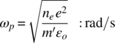
Figure 20.6 is a plot of the plasma frequency; ![]() , dependence on the electron density; and Table 20.7 tabulates and describes the parameters.
, dependence on the electron density; and Table 20.7 tabulates and describes the parameters.

FIGURE 20.6 Dependence of plasma frequency on electron density.
TABLE 20.7 Ionospheric Channel Parameters and Constants
| Parameter | Value | Unitsa | Description |
| N(ℓ) | Computed | Electrons/m3 | Electron density |
| ℓ | Computed | Meters | Distance along propagation path |
| ω, ωc | System parameters | Radians/second | Angular frequencyb |
| e | 1.602 × 10⁻¹⁹ | Coulombs/electron | Electron charge |
| εo | 8.854 × 10⁻¹² | Coulomb2second2/(Kg‐m3) | Free‐space permittivity (dielectric constant) |
| m′ | 9.109 × 10⁻³¹ | Kg/electron | Electron mass |
| ne | Channel parameter | Electrons/m3 | Electron density |
| Channel parameter | Electrons/cm3 | Electron density | |
| c | 2.997925 × 10⁸ | Meters/second | Free‐space velocity |
| v | 6.06 × 10⁶ at 50 km | Radians/second | Electron collision frequencyc |
| 1.75 × 10³ at 100 km | |||
| BT | Computed | Gauss | Transverse magnetic induction |
| BL | Computed | Gauss | Longitudinal magnetic induction |
| B | 0.5 | Webers/m2 | Magnitude of magnetic inductionc |
a mks system of units.
b In the following f denotes the frequency in hertz and fc denotes a selected carrier frequency.
c Numerical values based on the 1959 ARDC model atmosphere.
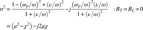
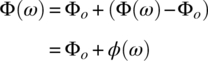
The refractive index is also characterized in terms of the complex quantity
Application of the index of refraction to a communication link yields the influence of the ionospheric propagation on the received signal. Consider, for example, a transmitted communication waveform expressed as eT(t) and after propagating a distance ℓ through a striated region of the ionosphere of path length L, the signal experiences an absorption and phase shift and is expressed as

The absorption coefficient κ is defined as
or, expressed in decibels, the absorption coefficient is 8.686κ dB/m. The signal phase shift introduced by the striated region gives rise to signal dispersion that is characterized by the channel phase constant denoted as β(ℓ) and expressed as
The dependence of the phase constant on the communication path length ℓ is explicitly shown for a constant electron density. However, as will be seen in Section 20.6, the fluctuations over the path through the striated region are characterized by the range‐dependent refractive index u(ℓ).
A general evaluation of the real and imaginary parts of Appleton’s expression is difficult; however, several simplifying assumptions provide insight into the channel behavior as well as practical characterizations of the received signal. The first of these assumptions is that the electron collision frequency is negligible, that is, ν/ω ≪ 1, and the second is that magnetic field effects are negligible, that is, B = 0.
20.4.1 Magnetic Field and No Electron Collisions
In this case it is assumed that the electron collision frequency is much less than the carrier angular frequency so the imaginary term jν/ω in Appleton’s expression is neglected leading to the result

Although this is a realistic result for satellite links operating above about 1 GHz, it is difficult to evaluate, in part, because the ± term in the denominator leads to ordinary and extraordinary waves, respectively, which are, to varying degrees, dependent on the strength and orientation of the magnetic field and the direction of propagation. A convenient expression results if the influence of the magnetic field is ignored as indicated in the following two sections.
20.4.2 No Magnetic Field and No Electron Collisions
If the magnetic field is neglected if BT = BL = 0 and the index of refraction reduces to the simplest form given by

20.4.3 No Magnetic Field with Electron Collisions
When the electron collisions are ignored the imaginary part of the index of refraction is zero so the absorption cannot be characterized in terms of the physical characteristics of the channel. However, to provide some insight into the absorption characteristics, it is convenient to ignore the effects of the magnetic field while permitting electron collisions. These conditions lead to the result
and equating the real and imaginary parts of these expressions yields
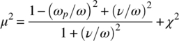
and

Solving for μ, using (20.16) and (20.17) under the condition ![]() results in the approximate expression
results in the approximate expression

The ellipsis in (20.18) represents neglected terms involving powers of (ωp/ω) and (v/ω) greater than four and two, respectively. The approximation applies when v ≪ ω which is a reasonable approximation when f > 100 MHz. Substituting (20.18) into (20.17), under the condition ![]() , the signal absorption term is approximated as
, the signal absorption term is approximated as

20.5 SIGNAL PROPAGATION IN SEVERE SCINTILLATION ENVIRONMENT
The principal parameters associated with scintillation in an ionized or striated channel are listed in Table 20.8.
TABLE 20.8 Principle Scintillation Dependent Parameters
| Parameter | Name | Description |
| S4 | Scintillation parameter | Typically: 0 ≥ S4 ≤ 1 |
| Rytov parametera | ||
| Electron variance | Over propagation path | |
| Signal phase variance | Over propagation path | |
| Energy angle‐of‐arrival variance | Results in antenna loss | |
| ℓo | Decorrelation length | Spatial correlation parameter |
| τo | Signal decorrelation time | Temporal correlation parameter |
| fo | Signal decorrelation bandwidth | Frequency‐selective bandwidth |
a This notation should not be confused with the imaginary part of the refractive index.
The most commonly used measure of signal fading is the S4 scintillation index defined as3

where V is the instantaneous rms signal voltage and the averaging time is much greater than the signal fade duration. The S4 scintillation index saturates at unity corresponding to severe scintillation with Rayleigh signal amplitude fading; but S4 index may exceed unity prior to saturation under some conditions. As discussed in Chapter 1, the Rayleigh amplitude pdf is characterized by independent quadrature Gaussian signals, N(0,σn), with a uniform phase pdf over 2π radians. Rayleigh scintillation may persist for many hours affecting communications over large geographical regions with longitude ground ranges listed in Table 20.9; the EHF band is sensitive to parameter uncertainties and may be less than indicated.
TABLE 20.9 Ground Range Extent Affected by Severe Scintillation
| Frequency Band | Longitude Ground Range (km) |
| EHF | 480 |
| X | 1600 |
| S | 2400 |
| L | 2570 |
| UHF | 3200 |
High altitude detonation, TAB = 30 min.
Because of the severity and extent of the scintillation, a robust communication system design must be capable to operating under severe scintillation conditions and, for this reason, the analysis, design, and system performance evaluations in Section 20.7 and following are based on a Rayleigh fading received signal. For S4 > 0.4 the Nakagami pdf4 is a good approximation to the amplitude fading statistics which is, theoretically, equal to the Rayleigh pdf when S4 = 1.0; however, S4 > 0.4 corresponds to severe scintillation and it is recommended that system designs be based on Rayleigh fading statistics when S4 > 0.4. As the scintillation index decreases the scintillation diminishes with S4 ≤ 0.4 corresponding to weak scintillation and, when S4 = 0, the received signal does not exhibit scintillation; however, the signal propagation is influenced by phase distortion‐related effects as discussed in Section 20.6.
The Rytov parameter is defined in terms of the parameters of the striated region and is approximated as [24]

where the scale sizes (Lz, Lx, Ly) form an orthogonal coordinate system that is dependent on the geomagnetic field lines,5 Lp is the propagation path length through the striated region, and fg is the carrier frequency in gigahertz. The parameter ![]() is the variance of the TEC (NT) expressed in (20.1). In the absence of an accurate estimate of the phase standard deviation, it is reasonable to use σe = NT. The condition
is the variance of the TEC (NT) expressed in (20.1). In the absence of an accurate estimate of the phase standard deviation, it is reasonable to use σe = NT. The condition ![]() results in severe scintillation so Rayleigh fading statistics are to be applied under this condition.
results in severe scintillation so Rayleigh fading statistics are to be applied under this condition.
In view of the uncertainty of parameters available in the open literature, the system design must be based on parametric performance evaluations. The uncertainties include the time‐dependent electron density profiles; the computation of the scintillation index S4 or ![]() ; the parameters
; the parameters ![]() ,
, ![]() , ℓo, τo, fo, and the signal losses Lscat, and La (described later). However, the recommendation that antiscintillation (AS) systems be designed to operate in the Rayleigh fading regime allowing the system design and performance evaluation to proceed based on specifications identifying the range of several parameters; most notability the electron density fluctuations, the channel decoration time (τo), and the frequency selective bandwidth (fo). Waveform and system mitigation techniques are described in Section 20.8.
, ℓo, τo, fo, and the signal losses Lscat, and La (described later). However, the recommendation that antiscintillation (AS) systems be designed to operate in the Rayleigh fading regime allowing the system design and performance evaluation to proceed based on specifications identifying the range of several parameters; most notability the electron density fluctuations, the channel decoration time (τo), and the frequency selective bandwidth (fo). Waveform and system mitigation techniques are described in Section 20.8.
In the following descriptions, the communication link is modeled as a one‐way path between a transmitting and receiving terminal with an ionized medium characterized as a plume of elections forming striations along the Earth’s magnetic field lines. The terminals are typically thought to be Earth or airborne terminals communicating with a satellite or satellites communicating over cross‐links. In general, the geometry is depicted as shown in Figure 20.7. In the evaluation of the communication link characteristics, the uplink and downlink asymmetry associated with Rgs ≠ Rss is important. The following description considers a nearly vertical communication link between a ground terminal and a geosynchronous satellite with altitude or range R = 35,784 km. The communication link passes through a striated medium resulting from a nuclear detonation at an altitude (range) of Rs = 400 km having an extent along the line of sight (LOS) path of Rse = 1000 km. Rse is considered to be symmetrical about Rs. Furthermore, consider that the lower altitude of the striated region is Rgs = 150 km. If the communication link corresponds to an uplink, the parameters in Figure 20.7 become: Gt = Gg, Rt = Rgs = 150 km, Gr = Gs, and Rr = Rss = R − Rgs − Rse = 34,634 km. Conversely, the communication downlink is evaluated by reversing the roles of the transmitter and receiver gains and ranges so that: Gt = Gs, Rt = Rss = 34,634 km, Gr = Gg, and Rr = Rgs = 150 km. These examples will be used to emphasize the impact of the direction of transmission on various design parameters.

FIGURE 20.7 Communication link encounter through striated region.
For strong localized scattering6 the square of the spatial decorrelation distance, ℓo, is expressed as [25]
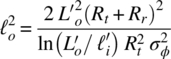
where the parameters Rt = Rgs and Rr = Rss are depicted in Figure 20.7 and ![]() is the variance of the carrier frequency phase over the range Rse through the striated region. In (20.22) the parameters
is the variance of the carrier frequency phase over the range Rse through the striated region. In (20.22) the parameters ![]() and
and ![]() represent the outer and inner scale sizes, respectively, normal to the propagation path through the striated region. These scales sizes are obtained through coordinate transformations from the geomagnetic field lines as described in APPENDIX 20A; the scale sizes in geomagnetic coordinates are depicted in Figure 20.5. Typically
represent the outer and inner scale sizes, respectively, normal to the propagation path through the striated region. These scales sizes are obtained through coordinate transformations from the geomagnetic field lines as described in APPENDIX 20A; the scale sizes in geomagnetic coordinates are depicted in Figure 20.5. Typically ![]() ranges from 1 to 10 km and
ranges from 1 to 10 km and ![]() is about 1/15‐th of
is about 1/15‐th of ![]() . In addition to the coordinate transformations resulting in
. In addition to the coordinate transformations resulting in ![]() and
and ![]() , (20.22) implicitly includes the transformation from the magnetic field coordinates to the LOS vector containing propagation path Lp that is used in the computation of
, (20.22) implicitly includes the transformation from the magnetic field coordinates to the LOS vector containing propagation path Lp that is used in the computation of ![]() . The implicit transformation factor K(Φ) is based on the penetration angle Φ between the geographic LOS path and geomagnetic field at the altitude of the strong localized scattering and is expressed as
. The implicit transformation factor K(Φ) is based on the penetration angle Φ between the geographic LOS path and geomagnetic field at the altitude of the strong localized scattering and is expressed as
The relationship to the signal phase variance is ![]() . The expression (20.22) for ℓo strictly applies for unit‐gain omnidirectional transmit and receive antennas, in which case, the variance of the signal energy angle‐of‐arrival is expressed as
. The expression (20.22) for ℓo strictly applies for unit‐gain omnidirectional transmit and receive antennas, in which case, the variance of the signal energy angle‐of‐arrival is expressed as

where λ is the wavelength of the signal carrier frequency. The angle σθ is a measure of the angular deviation of the received multipath signal rays from the LOS path.
It is evident from (20.22) that ℓo is dependent upon the direction of transmission. For example, referring to Figure 20.7 and the conditions of the previous example, suppose that Rt = Rss = 34,634 km with Rt + Rr = 34,784 km corresponding to a downlink transmission. In the case of an uplink transmission Rt + Rs remains the same however Rt = Rgs = 150 km so the value of ℓo increases by a factor of about 232 : 1.
The signal decorrelation time is given by
where V = Vpr + VT. The velocity Vpr is the velocity of the plasma or striated region and VT is the terminal velocity contributions, where both are in the plane of the receive antenna. The plasma velocity is computed as

where VM is the magnitude of the plasma velocity normal to the LOS propagation path and aligned with the plane of the receiver. Considering the plasma velocity vector in the magnetic field plane (MFP) to be ![]() , the plasma velocity normal to the LOS is computed as
, the plasma velocity normal to the LOS is computed as

Typically the magnitude of the plasma velocity in the MFP is VM = 1–20 km/s. The first transformation in (20.27) is evaluated in APPENDIX 20A and results from the transformation of the geomagnetic polar coordinates (Φ,Λ) to the geographic polar coordinates (φ, λ) of a point in space Px. The second transformation is required to rotate geographic coordinates of point Px into alignment with the propagation path.
Using the expression (20.22) for ℓo and neglecting the terminal velocity, the decorrelation time is evaluated as

From (20.28) it is evident that τo is independent of the direction of transmission. The frequency‐selective bandwidth is also dependent on ℓo through the following relationship [26]

The last expression results with the constant C1 = 0.25; this is a practical constant bound for the relatively small effect of the time delay jitter and results in the scintillation being a function only of τo and fo [27]. Upon substituting (20.22) for ![]() into (20.29) the frequency‐selective bandwidth is expressed as
into (20.29) the frequency‐selective bandwidth is expressed as

From (20.29) and (20.30) it is seen that fo is dependent on the direction of transmission.
Estimates of reasonable worst‐case ranges [23] of the signal decorrelation time and decorrelation bandwidth are shown, respectively, in Figures 20.8 and 20.9 as a function of the carrier frequency. The shaded areas correspond to the most severe or Rayleigh scintillation that transitions through Ricean scintillation to the channel conditions prior to the nuclear detonation. Depending on the geometry of the encounter, a blackout regime may be encountered prior to the Rayleigh regime. The blackout regime is generally defined as the time following the detonation when the received signal level is greater than 3 dB below the mean level of the Rayleigh fading signal. The signal decorrelation time and the frequency decorrelation bandwidth are defined as the point that the respective normalized correlations fall to e−1 of the peak correlation; these correlation responses are also referred to as the channel correlation responses.

FIGURE 20.8 Reasonable worst‐case channel decorrelation times.
McDaniel [23]. Reproduced with permission of the Defense Threat Reduction Agency (DTRA).

FIGURE 20.9 Reasonable worst‐case channel decorrelation bandwidth (frequency‐selective bandwidth).
McDaniel [23]. Reproduced with permission of the Defense Threat Reduction Agency (DTRA).
The channel decorrelation time τo and the decorrelation bandwidth (or frequency‐selective bandwidth) fo are the two most influential channel parameters in the selection of the waveform and the system designs. For example, the channel fade rate is defined as Rf = 1/τo and slow and fast fading corresponds to large and small values of τo, respectively.7 For reliable communications the communication systems must operate over the entire range of τo at the specified carrier frequency as shown in Figure 20.8. The range of decorrelation times places an increasingly heavy burden on the waveform selection and design of FEC coding, interleaving, and combining as the information rate increases; in some cases it may be prudent to use message repetition and combining.
If the instantaneous bandwidth of a transmitted symbol exceeds the decorrelation frequency fo the signal will experience frequency‐selective fading in which regions of the signal spectrum become uncorrelated resulting in severe signal distortion. However, if the signal bandwidth is sufficiently less than fo, the entire spectrum is affected in the same way resulting in frequency‐nonselective fading. With frequency‐nonselective fading, signal FEC coding, interleaving, and combining are effective mitigations techniques.8 Although it is always prudent to verify the performance using computer simulations, they are particularly important when the channel fading lies between frequency selective and nonselective regimes.
20.5.1 Impact on Directive Antenna Gain
The previous expression for ℓo and consequently those for τo and fo are based on an ideal unit‐gain isotropic radiator. When practical antennas are considered, that is, antennas exhibiting a directive gain, the expression for the correlation distance at the output of the receiver antenna is evaluated as [28]

where Gt and Gr are the gains of the transmit and receive antennas and the factor (Rr/Rt)2 projects the aperture of the transmit antenna onto the plane of the receive antenna. The gain is given by ![]() and, for a parabolic dish antenna with radius r and efficiency ηa, the effective antenna aperture is given by
and, for a parabolic dish antenna with radius r and efficiency ηa, the effective antenna aperture is given by ![]() . The designation
. The designation ![]() is used to denote the correlation distance at the output of the receive antenna. The energy angle‐of‐arrival is defined as the angle, relative to the receiver antenna LOS axis, of the received signal emerging from the striated region. The standard deviation of the energy angle-of-arrival is given by
is used to denote the correlation distance at the output of the receive antenna. The energy angle‐of‐arrival is defined as the angle, relative to the receiver antenna LOS axis, of the received signal emerging from the striated region. The standard deviation of the energy angle-of-arrival is given by

Using this result, ![]() is expressed in terms of the variance of the energy angle‐of‐arrival as
is expressed in terms of the variance of the energy angle‐of‐arrival as

where ![]() is defined as the energy angle‐of‐departure from the transmit antenna and is given by
is defined as the energy angle‐of‐departure from the transmit antenna and is given by

The signal decorrelation time and bandwidth and the antenna loss are impacted by the antenna directional gain in a similar manner. Upon substituting the channel decorrelation length ![]() into expressions (20.22) and (20.25) for τo and fo, respectively, the corresponding expressions for
into expressions (20.22) and (20.25) for τo and fo, respectively, the corresponding expressions for ![]() and
and ![]() at the receiver antenna output terminals are evaluated as
at the receiver antenna output terminals are evaluated as

and

Although τo is not dependent on the direction of transmission, because of the different antenna gains and the asymmetry of the striated region along the transmission path, ![]() is dependent on the direction of the transmission.
is dependent on the direction of the transmission.
The antenna loss at the receiver, resulting from the Gaussian distributed ray scattering through the medium, is expressed as [26]

Equation (20.37) is defined as the antenna scattering loss and must be combined with the absorption loss along the propagation path.
20.5.2 Ionospheric Absorption
The signal absorption loss through the ionosphere is evaluated using (20.10) as
or, upon substituting for χ using (20.19), which applies for v ≪ ω, and expressing the absorption loss in terms of decibels, the signal absorption loss is evaluated as

where9 the second expression uses (20.8) to substitute for ![]() and the last expression substitutes the constant values from Table 20.7. Upon expressing the electron collision frequency profile in (20.6) in terms of the height h above the Earth’s surface, (20.39) becomes
and the last expression substitutes the constant values from Table 20.7. Upon expressing the electron collision frequency profile in (20.6) in terms of the height h above the Earth’s surface, (20.39) becomes

where f(h) is a unit‐less function of the height dependence on the antenna elevation angle θe as expressed by [5]

The total signal loss due to the medium and the antenna scatter power losses is
The absorption loss in the natural environment, based on the Chapman electron density profiles, is given in Table 20.2. The electron collision profiles are listed in Table 20.5 and plotted in Figure 20.10 for carrier frequencies of 100 and 500 MHz under daytime and nighttime conditions. The loss is negligible at nighttime for frequencies greater than 100 MHz and at daytime for frequencies greater than 500 MHz.

FIGURE 20.10 Absorption loss in natural environment (Chapman model with solar zenith angle = 0°).
The mean electron densities (ne) given in Table 20.3 are used to evaluate the losses and the corresponding variations (σe) are used to compute the associated confidence levels based on the Gaussian distributed loss variations denoted as N(ne,σe). The losses at a carrier frequency of 100 MHz and corresponding confidence levels are tabulated in Table 20.10 for the equatorial, mid‐to‐low latitude, and Polar Regions. A major source of uncertainty in computing the absorption loss is determining the value of the collision frequency. The greatest impact of the collision frequency on the absorption loss is in the lower ionospheric regions from about 50 to 120 m and, as the altitude increases, the collision frequency has a diminishing effect on absorption.
TABLE 20.10 Absorption Losses (dB) in Natural Environment at 100 MHz
| Latitude | |||||
| Equatorial | Mid‐to‐Low | Polar | |||
| Confidence (%) | Turbulent | Moderate | Turbulent | Turbulent | Moderate |
| 50a | 5.75 | 2.88 | 0.95 | 5.10 | 2.55 |
| 90 | 28.52 | 4.77 | 1.08 | 19.57 | 3.76 |
| 95 | 35.10 | 5.32 | 1.11 | 23.75 | 4.11 |
| 99 | 47.19 | 6.33 | 1.18 | 31.43 | 4.77 |
a For mean or average electron density.
Referring to (20.40), the absorption loss scales inversely proportional to the square of the frequency; therefore, defining the losses in Table 20.10 as La(100 MHz)dB, the loss at an arbitrary frequency, expressed in megahertz, is determined as

20.5.3 Receiver Noise
The receiver noise is impacted by the increase in the receiver antenna noise temperature as a result of the fire ball from the detonation. The antenna noise is dependent beam width and the propagation LOS relative to the location of the detonation and is expressed as [29]
where TFB is the fireball temperature on the order of 1000°K and ![]() is the propagation loss over the path between the fireball and the receiver.
is the propagation loss over the path between the fireball and the receiver.
20.6 PROPAGATION DISTURBANCES FOLLOWING SEVERE ABSORPTION
The initial impact of a nuclear detonation on a communication link is a severe signal attenuation that may exceed several minutes in duration depending upon the operating frequency and the link path relative to the fireball of the detonation. This is referred to as the signal blackout regime and the only effective mitigation techniques are spatial diversity that uses another link path that is not impacted by the fireball. However, increasing the carrier frequency is only advantageous because of the lower absorption loss and susceptibility to scintillation following the severe fireball temperatures. As the blackout regime subsides, the signal level begins to recover and enters the scintillation regime. During the scintillation regime, the signal absorption has essentially diminished so that communications can resume if the underlying communication waveform is properly designed to mitigate the signal scintillation. In the scintillation regime, the received signal level fluctuations, or fading, results from carrier frequency phase constructive and destructive interference that cannot be overcome by increasing the power. This is an especially important concept in the design of frequency and time diversity waveform mitigation techniques. Therefore, because it is impractical to increase the signal power to overcome the increase in the system noise temperature resulting from the fireball or to overcome the signal phase cancellation effects, it is recommended that a 3 dB link margin be provided to aid in the link recovery during the transition to the scintillation regime with the principal mitigation techniques embodied in the network protocol and waveform design as discussed in Section 20.8.
Therefore, in this section, severe signal absorption is assumed to have subsided and the electron density of the ionosphere is considered to have a slowly varying average value with a diminishing, electron density variation about the mean value. In this regime the signal scintillation is referred to as resulting from phase‐only affects; however, the signal amplitude continues to fluctuate about the mean value of the Rayleigh distribution with a uniformly distributed phase. By considering the time dependence of the TEC either resulting from changes in the communication path or the electron density fluctuations along the path, the impact of time‐varying ISI on the communication system performance is evaluated. In this context, the channel impulse response is examined and the resulting ISI is characterized in terms of the modulated waveform symbol rate. Based on these considerations, the analysis in this section involves traditional multipath phenomenon using the parameters identified in Table 20.11.
TABLE 20.11 Multipath Related Parameters
| Parameter | Name | Description |
| Td | Free‐space delay | |
| td | Delay through striated region | Additional delay to free‐space delay |
| Td1 | Quadratic delay distortion | Dispersion delay causing signal distortion |
| Td2 | Cubic delay distortion | Dispersion delay causing signal distortion |
| fd | Doppler | Doppler spread |
| Absorption loss (dB) | Path loss through striation region | |
| Ta | Antenna temperature | Increase due to elevated temperature of plasma |
| θf | Faraday rotation | Linear polarization phase change |
For this analysis the channel frequency response is characterized as
where ω is the instantaneous angular frequency. Considering the length of the communication path through the striated region of the ionosphere to be L meters, the channel phase function is evaluated as

where ![]() is the channel phase constant. For the previous simplifying assumptions, the real part of the refractive index is expressed by (20.14) as
is the channel phase constant. For the previous simplifying assumptions, the real part of the refractive index is expressed by (20.14) as
The change in the channel phase relative to that of free‐space propagation, that is, for ![]() , results in the phase function
, results in the phase function
where ![]() and Lp is the undisturbed propagation path length. The phase function through the disturbed region with path length L is expressed as
and Lp is the undisturbed propagation path length. The phase function through the disturbed region with path length L is expressed as

Expanding the radical in the integrand of (20.49) in terms of a power series with ω > ωp results in the approximation

This approximation ignores the higher order terms: −(ωp/ω)4/8 − (ωp/ω)6/16 − ⋯. Expanding the function f(ω) = 1/ω in (20.50) using a Taylor series about the carrier frequency ωc results in

Referring to (20.8), the integral in (20.51) is evaluated as

where the dimension of ![]() is expressed in radians2/second2. The last approximation assumes that the electron density is the average (or a weighted average) over the path length L. This is a reasonable assumption over short time intervals since there are no electron collisions and the electron plume is expanding from the force of the detonation and later contracting through electron recombining in the troposphere and lower ionosphere. Both of these events occur over relatively long periods of time compared to the typical communications message duration and snapshots of the electron profiles can be predicted. It is recommended that AS systems are to be designed for the worst‐case scenario which favors the weighted average being biased toward the worse‐case electron density. However, laying these details aside, in the following analysis the performance of the communication system is evaluated parametrically in terms of the plasma frequency
is expressed in radians2/second2. The last approximation assumes that the electron density is the average (or a weighted average) over the path length L. This is a reasonable assumption over short time intervals since there are no electron collisions and the electron plume is expanding from the force of the detonation and later contracting through electron recombining in the troposphere and lower ionosphere. Both of these events occur over relatively long periods of time compared to the typical communications message duration and snapshots of the electron profiles can be predicted. It is recommended that AS systems are to be designed for the worst‐case scenario which favors the weighted average being biased toward the worse‐case electron density. However, laying these details aside, in the following analysis the performance of the communication system is evaluated parametrically in terms of the plasma frequency ![]() .
.
Substituting (20.52) into (20.51) results in the approximate channel phase expression

Referring again to (20.8), characteristic frequency of the plasma is evaluated as

Using these results, the phase function in (20.48) is expressed as

It is convenient to characterize the phase function about the carrier frequency by defining10 ![]() and, upon substitution into (20.55), the low‐pass phase function is expressed as
and, upon substitution into (20.55), the low‐pass phase function is expressed as

where Φo is evaluated using the relationship ![]() . The linear phase term in u simply represents a constant delay and the higher order terms contribute to the signal distortion.
. The linear phase term in u simply represents a constant delay and the higher order terms contribute to the signal distortion.
20.6.1 Signal Delay and Dispersion
Considering the channel phase function Φ(u), the resulting signal delay function is given by

The constant delay, resulting from the LOS path, is given by To = Td + td where Td = Lp/c is the delay from the undisturbed channel and, with TL = L/c, the delay over the path L through the disturbed channel is evaluated using

These delays do not result in signal distortion; however, the quadratic and higher order frequency‐dependent delay terms result in signal distortion. The linear and quadratic delay terms are evaluated as

and

Expressing the frequency deviation from the carrier as Δf = u/2π Hz and normalizing these delays by the symbol duration, the normalized delay distortion terms become

and

20.6.2 Example of Signal Delay Distortion
In this example, the delay terms through the linear distortion term are considered, that is, the higher order distortion terms are neglected, so the channel frequency response is characterized as
where ![]() is the angular frequency about the carrier frequency. Referring to (20.48) the phase φo is evaluated as
is the angular frequency about the carrier frequency. Referring to (20.48) the phase φo is evaluated as

and from (20.57) To is evaluated as


The channel impulse response is evaluated using the inverse Fourier transform as

where W is the radio frequency (RF) bandwidth centered on the carrier frequency fc. In this analysis the magnitude of the channel impulse response is evaluated in terms of Fresnel integrals as [30]

The upper and lower integration limits z2 and z1 of the Fresnel integrals are expressed as

These results are normalized by letting y = tW, ![]() , and
, and ![]() . Using these results the magnitude of the channel impulse response is evaluated in terms of the normalized parameters as
. Using these results the magnitude of the channel impulse response is evaluated in terms of the normalized parameters as

and the normalized arguments of the Fresnel integrals are expressed as

The channel impulse response simulation results, shown in Figure 20.11, correspond to yo = 0, a path length of L = 1 km through the ionized medium, a carrier frequency of fc = 10 GHz, and a normalized bandwidth parameter of W/fc = 2e−7, which corresponds to a channel symbol rate of Rs = 2k symbols/s. The nonideal impulse response depicts the pulse dispersion caused by the quadratic phase distortion that is a direct result of the TEC (electrons/m2) through the disturbed region. The results apply to noncoherent (NC) symbol detection and the range 1e11 ≤ TEC ≤ 1e12 corresponds to those found in the natural environment. By way of comparison, for carrier frequencies of 60 and 300 GHz the respective TEC ranges are 1e13 ≤ TEC ≤ 1e14 and 6e15 ≤ TEC ≤ 1e16. The ISI must be evaluated further by examining the correlation response of the detection filter; however, the impact on the symbol‐error performance must be examined using additional analysis or Monte Carlo simulations. These evaluations should include mitigation techniques including adaptive ISI cancellation and FEC. In this regard, this analysis has limited utility and may be considered as a first step in characterizing the impact of the TEC on the communication link performance. Although considerably more involved, this analysis can also be extended to initially examine the impact of the TEC on coherent detection and phaselock loop tracking.

FIGURE 20.11 Ionospheric channel impulse response characteristics (L = 1 km, fc = 10 GHz, Rs = 2k symbols/s).
20.7 RAYLEIGH SCINTILLATION CHANNEL MODEL
The amplitude variations or scintillation of a received signal propagating through a heavily ionized region of the ionosphere is the result of the constructive and destructive interaction of the signal phase resulting from numerous signal paths through the media. The phenomena of scintillation are described in Sections 20.2 and 20.3 that includes example electron density profiles for natural and nuclear‐disturbed environments. In addition to the electron density concentrations, the dynamics of the channel and communication system will further influence the scintillation characteristics of the received signal.
Because the predominant influence of the media is upon the signal phase, the channel is characterized in terms of a phase power spectral density (PPSD) function. The analysis described in this section to characterize the received signal scintillation was proposed by Wittwer [31] and provides a relatively straightforward way to generate receiver amplitude and phase perturbations in a Rayleigh environment corresponding to severe scintillation. An alternate approach to that presented in this section is discussed by Knepp [32]. Using the PPSD also allows for generating receiver amplitude and phase fluctuations having correlation properties directly related to the physical parameters of the environment. The PPSD of interest, obtained from extensive research involving the modeling of observed phenomena [33], is expressed as

The variable ![]() is the spatial angular frequency and λ represents the spatial wavelength. The parameter ξ is the spatial frequency having units of cycles/meter and Lo is referred to as the outer scale size and represents the length of the electron homogeneity in the structured ionosphere. This scale size ranges from 1 to 10 km and, as will be seen, is related to the spatial correlation length ℓc in the plain of the receiver.
is the spatial angular frequency and λ represents the spatial wavelength. The parameter ξ is the spatial frequency having units of cycles/meter and Lo is referred to as the outer scale size and represents the length of the electron homogeneity in the structured ionosphere. This scale size ranges from 1 to 10 km and, as will be seen, is related to the spatial correlation length ℓc in the plain of the receiver.
The parameter ![]() is the signal phase variance and is related to the electron density fluctuation [34]
is the signal phase variance and is related to the electron density fluctuation [34] ![]() . However, because the present analysis is concerned with Rayleigh amplitude statistics, the intensity fluctuation is, in a sense, saturated and
. However, because the present analysis is concerned with Rayleigh amplitude statistics, the intensity fluctuation is, in a sense, saturated and ![]() simply becomes a scale factor. Expressed as a function of the spatial frequency ξ, the PPSD is given by
simply becomes a scale factor. Expressed as a function of the spatial frequency ξ, the PPSD is given by

The electric field fluctuation in the plain of the receiver11 is obtained by taking the inverse Fourier transform of the zero‐mean complex Gaussian random variable
where the quadrature components i = {I,Q} are distributed as

with variance ![]() . The components b i(ξ) are statistically independent in i and ξ.
. The components b i(ξ) are statistically independent in i and ξ.
Based on these characterizations, the received spatial electric field strength is given by

To generate receiver sample functions or sequences for use in subsequent system simulations, the inverse FFT is used and the discrete form of (20.76) is expressed as

where the n and m indices are defined as ![]() and ξ = nΔξ : n = 1,…,N. Furthermore, using a radix‐2 FFT of length N samples such that N is a power of two, results in
and ξ = nΔξ : n = 1,…,N. Furthermore, using a radix‐2 FFT of length N samples such that N is a power of two, results in ![]() . The quadrature components of the complex function
. The quadrature components of the complex function ![]() are also iid zero‐mean Gaussian random variables.
are also iid zero‐mean Gaussian random variables.
The 3‐dB spatial frequency of the PPSD, normalized to ![]() , is evaluated as
, is evaluated as ![]() and the spatial sampling frequency is
and the spatial sampling frequency is ![]() , where K is selected to satisfy the Nyquist criterion. Figure 20.12 shows the sampling characteristics of the three functions of interest with the abscissa expressed in terms of the outer scale size Lo. Figure 20.13 shows a typical computed spatial sequence (or record) for Lo = 3 km,
, where K is selected to satisfy the Nyquist criterion. Figure 20.12 shows the sampling characteristics of the three functions of interest with the abscissa expressed in terms of the outer scale size Lo. Figure 20.13 shows a typical computed spatial sequence (or record) for Lo = 3 km, ![]() , with K = 64 and N = 4096.
, with K = 64 and N = 4096.

FIGURE 20.12 Representations of spectral and spatial functions.

FIGURE 20.13 Typical computer‐generated receiver spatial sequence.
20.7.1 Spatial Correlation of Receiver Electric Field Strength
The correlation distance ℓo of the receiver electric field is a significant parameter and is used to determine the required separation between receiver terminals for spatial combining diversity. It is also used to determine the scintillation decorrelation time τo used to determine FEC code length, interleaver length, and repeat message intervals for temporal combining. The correlation distance is defined in terms of the normalized autocorrelation coefficient ![]() such that
such that
The correlation function R(ℓ) is evaluated as
Evaluation of (20.79) using the expression for εk proceeds as follows:

Because bn and ![]() are orthogonal, that is, are independent normal random variables,
are orthogonal, that is, are independent normal random variables, ![]() , where δnm is the Kronecker delta function. Using this result the correlation function becomes
, where δnm is the Kronecker delta function. Using this result the correlation function becomes

Using the expression for the complex iid zero‐mean samples bn results in

and the desired expression for the correlation function becomes

Equation (20.83) is evaluated numerically to determine the correlation distance ℓo or by changing the integrand to a continuous function, normalizing by R(0) and evaluating the resulting integral yields the normalized solution

where K1(–) is the modified Bessel function of order one. Evaluation of this result at the decorrelation value of e−1 results in the correlation distance
To check the fidelity of the simulation code in generating the sampled received electric field sequences, the correlation responses of the sequences shown in Figure 20.13 are evaluated and the results are shown in Figure 20.14 with the abscissa plotted in terms of the spatial distance ![]() , m = 1,…, N − 1. From these results and using the decorrelation value of 0.368 defined earlier, the correlation distance for both the in‐phase and quadrature channels are nearly the same and equal to
, m = 1,…, N − 1. From these results and using the decorrelation value of 0.368 defined earlier, the correlation distance for both the in‐phase and quadrature channels are nearly the same and equal to ![]() . The theoretical value, derived earlier is ℓo = 1.65(3 km) = 4.95 km so the simulated results are within 7.4% of the theoretical value. As the number of independently generated received sequences increases the average correlation response converges to the theoretical response expressed by (20.83).
. The theoretical value, derived earlier is ℓo = 1.65(3 km) = 4.95 km so the simulated results are within 7.4% of the theoretical value. As the number of independently generated received sequences increases the average correlation response converges to the theoretical response expressed by (20.83).

FIGURE 20.14 Correlation characteristics of simulated receiver sequence.
As a further verification of the simulation code, the power spectral density of the received field strength is computed and shown in Figure 20.15. The circled data points represent the PPSD based on the simulation results in Figures 20.13 and 20.14; the solid curves in Figure 20.15 are the theoretical PPSD. To obtain a quantitative measure of the simulated PPSD results a linear mean‐square regression analysis is computed for the samples in Figure 20.15b in the range 0.2 ≤ ξ ≤ 2.17. This analysis indicates that slope of the PPSD curve and 3 dB intercept point are within 3.6 and 4.5% of the respective theoretical values.

FIGURE 20.15 Reconstructed PPSD based on the simulation‐generated sequences of the receiver electric field strength.
20.7.2 Concatenation of Computer‐Generated Scintillation Records
In this and the following section, the independently generated orthogonal receiver electric field strength sequences described in the preceding section are stored as data records and used as required in a system simulation. Typically a system simulation will require the concatenation of many data records over the time spanned by the communication data or message. Each data record is generated using different noise seeds so the in‐phase and quadrature scintillation samples in each record and between the records are independent. To concatenate data records in a seamless manner without severe amplitude and phase discontinuities, the records to be joined are separated in distance by one correlation interval (ℓo) and interpolation is used to generate additional samples to fill‐in the gap of length ℓo. The interpolation is based on a third‐degree polynomial in ℓ with coefficients computed based on the boundary conditions yielding equal amplitude and slopes of the two records being joined. This is equivalent to solving the equation

where εo is the last data point in the current record, assumed to be at ℓ = 0 and ε1 is the first data point in the new record, assumed to be at ℓ = ℓo. The primed values are the slopes of the corresponding data points that are computed using the next to the last and the second data point in the respective records. The number of data points used to span the correlation interval ℓo is ![]() .
.
20.7.3 Spatial‐to‐Temporal Conversion of Computer‐Generated Data Records
In this section, the application of the spatial data records to the received signal data‐modulated waveform is described. The first step involves the conversion of the spatial sequences to temporal sequences based on the knowledge of the dynamics of the electron plume and the communication platform. If the encounter were completely stationary, that is, the communication platforms were fixed in position and the Earth’s rotation and electron plume were frozen in place, then the received signal amplitude would be based on a random selection from the Rayleigh amplitude distribution. If, however, the selected amplitude resulted in a deep amplitude null, exceeding the available link margin then communications would be impossible. In this situation if, for example, the receiver were to move by about one spatial correlation interval ℓo, then it would be likely that the resulting signal amplitude would be high enough of to establish communications. The phenomena of this idealized example is exactly what is taking place; however, the Earth and electron plume is continually moving and the communication platforms themselves exhibit velocity components that contribute to the Rayleigh received signal amplitude fluctuations. During the time immediately following the detonation, the electron plume will exhibit extremely high velocity components due to the forces of the initial blast. Following the initial detonation, the energy dissipates resulting in less dynamic interactions and lower velocities. During this period of electron recombining in the ionosphere and troposphere much longer lasting scintillation effects continue due to the influence of wind and other natural dynamic forces that influence the direction and velocity of the electron plume.
The velocity of interest is the velocity vector in the plane of the receiver that results from all of the relative motions of the encounter. For example, consider that the resulting velocity in the plane of the receiver is ![]() , where ℓ is the distance that a point on the received spatial sequence moves in t seconds. As mentioned previously, the time for this fictitious point to move one correlation interval of length ℓo is defined as the temporal decorrelation time τo, so that, the velocity is described as
, where ℓ is the distance that a point on the received spatial sequence moves in t seconds. As mentioned previously, the time for this fictitious point to move one correlation interval of length ℓo is defined as the temporal decorrelation time τo, so that, the velocity is described as
Using the right‐hand equality in this expression and substituting for the correlation distance in terms of Lo results in the normalized expression
The maximum time spanned by a computer‐generated sequence is determined from the maximum length ℓmax and, referring to Figure 20.12, ![]() so that
so that
Using the example parameters: N = 4096, K = 64 and Lo = 3 km, the number of decorrelation time constants spanned by a computer‐generated record is ![]() . This is an important consideration, in that, the accuracy and resulting confidence of a Monte Carlo performance simulation must take into account the relatively long times involved in characterizing the impact of the channel fluctuations. The corresponding sampling interval of the computer‐generated records is
. This is an important consideration, in that, the accuracy and resulting confidence of a Monte Carlo performance simulation must take into account the relatively long times involved in characterizing the impact of the channel fluctuations. The corresponding sampling interval of the computer‐generated records is

where the link between τo and ℓo is through the velocity, that is, ![]() . In terms of the computer‐generated records, referring to Figure 20.12c, the sample interval is
. In terms of the computer‐generated records, referring to Figure 20.12c, the sample interval is
Consider that a modulated symbol of duration T seconds (Rs = 1/T symbols/s) is received and sampled using Ns samples per symbol. Under these conditions, the required receiver sampling interval is
Except for the unique case when ![]() , it will be necessary to interpolate between the scintillation record samples and the required receiver sampling instant. To aid in the description of the sampling, Figure 20.16 shows the temporal samples (gk) that have been transformed from the spatial samples (εm) as described earlier. For convenience gk is considered to be a real signal and it is implicit that sampling and interpolation is applied to both the real and imaginary parts of the complex scintillation process. The interpolation of the symbol sample is based on linear interpolation. For example, considering kΔts ≤ iΔTs ≤ (k + 1)Δts the symbol sample gi corresponding to iΔTs is computed using the nearest record samples kΔts and (k + 1)Δts as
, it will be necessary to interpolate between the scintillation record samples and the required receiver sampling instant. To aid in the description of the sampling, Figure 20.16 shows the temporal samples (gk) that have been transformed from the spatial samples (εm) as described earlier. For convenience gk is considered to be a real signal and it is implicit that sampling and interpolation is applied to both the real and imaginary parts of the complex scintillation process. The interpolation of the symbol sample is based on linear interpolation. For example, considering kΔts ≤ iΔTs ≤ (k + 1)Δts the symbol sample gi corresponding to iΔTs is computed using the nearest record samples kΔts and (k + 1)Δts as


FIGURE 20.16 Temporal scintillation record sampling (solid lines) and interpolated samples (dashed lines).
The slow and fast scintillation conditions are defined in terms of the decorrelation time relative to the symbol duration. For the slow fading condition shown in Figure 20.16a, there are typically many symbol samples relative to the record samples and the parameters of the interpolation gk and gk+1 are not updated very often. For very slow scintillation, the record samples or symbol amplitudes are virtually constant over many symbols leading to a considerable saving in simulation time. In the case of fast scintillation, the record sampling must ensure that the symbol sampling does not result in aliasing. This can be accomplished by selecting the symbol sampling frequency fs such that fs = max(1/Δts, 1/ΔTs) where ![]() and
and ![]() is the required samples per symbol to satisfy the Nyquist sampling frequency in the additive white Gaussian noise (AWGN) channel. Using this and the previous results the required sampling frequency with scintillation can be expressed as
is the required samples per symbol to satisfy the Nyquist sampling frequency in the additive white Gaussian noise (AWGN) channel. Using this and the previous results the required sampling frequency with scintillation can be expressed as

Although not necessary, it is often convenient to choose the number of samples per symbol to be an integer in which case the condition ![]() applies and
applies and

where ![]() signifies the ceiling or the smallest integer greater than the argument and, in this case, is the required samples per symbol to satisfy the Nyquist condition with channel scintillation. For a given scenario the ratio ΔTs/Δts in the interpolation equation is a constant and, in view of the preceding comments, is generally expressed as
signifies the ceiling or the smallest integer greater than the argument and, in this case, is the required samples per symbol to satisfy the Nyquist condition with channel scintillation. For a given scenario the ratio ΔTs/Δts in the interpolation equation is a constant and, in view of the preceding comments, is generally expressed as

In the last equality of (20.96), the symbol sampling frequency is equal to the scintillation record sampling frequency and no interpolation is necessary. In this case, the channel symbol sampling frequency must be increased so that ΔTs = Δts and rate conversion or downsampling in the receiver processing may be applied to result in a convenient number of samples per symbol for demodulation and tracking. Of course, the rate conversion must satisfy the Nyquist sampling criterion in consideration of the received signal and channel bandwidths.
20.7.4 Additional Simulation Considerations
Upon inclusion of the signal scintillation data records described earlier into a simulation program, it is necessary to establish and verify various operational conditions to ensure reliable and accurate results. Several parameters requiring calibration and verification are discussed in this section.
20.7.4.1 Establishing the Receiver Signal‐to‐Noise Ratio
The Rayleigh fading channel introduces absorption and other losses that result in a net loss in the received signal power relative to the AWGN channel. The simulation code, however, does not need to account for these detailed losses as long as the received signal‐to‐noise ratio is properly established. In fact, because of various normalizations, the Rayleigh fading records result in a net channel gain that must be determined to establish the received signal‐to‐noise ratio. The power gain through the Rayleigh fading channel is simply the second moment of the Rayleigh pdf and is given by
where ![]() is the variance of the underlying Gaussian noise process used to generate the Rayleigh samples. For a finite‐length record, the channel power gain will vary from record to record and Table 20.12 lists the statistical parameters associated with five records each with 2048 complex samples εm. The received signal‐to‐noise ratio in an AWGN channel is computed as
is the variance of the underlying Gaussian noise process used to generate the Rayleigh samples. For a finite‐length record, the channel power gain will vary from record to record and Table 20.12 lists the statistical parameters associated with five records each with 2048 complex samples εm. The received signal‐to‐noise ratio in an AWGN channel is computed as ![]() where P is received signal power and
where P is received signal power and ![]() is the AWGN power. Therefore, the received signal‐to‐noise ratio from the scintillating channel is determined as
is the AWGN power. Therefore, the received signal‐to‐noise ratio from the scintillating channel is determined as
where ρ = E[|εm|2] = 504.607 is the average of five independently generated scintillation data records12 as listed in Table 20.12.
TABLE 20.12 Computed Parameters for Five Typical Rayleigh Scintillation Records
| Record | E[|εm|2] | E[|εm|] | σ[|εm|] |
| 1 | 463.47 | 19.116 | 9.902 |
| 2 | 502.793 | 19.892 | 10.349 |
| 3 | 555.349 | 20.850 | 10.983 |
| 4 | 489.232 | 19.448 | 10.536 |
| 5 | 512.193 | 20.234 | 10.138 |
| Composite results | |||
| All | 504.607 | 19.908 | 10.383 |
20.7.4.2 Generating Uncorrelated Samples
When performing a simulation it may be necessary to evaluate the received symbols under independent or uncorrelated fading conditions. This requirement applies, for example, with frequency hopping where groups of transmitted symbols are associated with each hop interval and the frequency hopping is greater than the channel correlation bandwidth fo. In these situations the scintillation record is run‐up or advanced by one correlation interval between each frequency hop thus simulating an uncorrelated scintillation condition from hop to hop. To achieve this result the scintillation record must be advanced by Nso samples where

For the example records discussed previously K = 64 so Nso = 13.
20.7.4.3 Verifying Record Generation
As in all simulations, it is necessary to evaluate the simulation code before committing to lengthy system performance runs. A convenient check of the channel sampling relative to the modulated symbol is to choose the number of channel samples to be equal to the Nyquist samples that are required to avoid aliasing in the AWGN channel. That is, by choosing
Or alternately by choosing
the symbol samples will correspond to the scintillation record samples which are easily verified.
20.8 SCINTILLATION MITIGATION TECHNIQUES
The techniques used to mitigate communications signal scintillation involve the system operating conditions, medium access control (MAC) protocols, and waveform design. The applicable mitigation techniques depend on the system mission requirements, for example, multiple links and satellites, selection of satellite orbits, ground support systems, communication networks and protocols, long transmissions involving video and mapping data, and short emergency action messages (EAMs). The waveform mitigation techniques include time diversity, FEC coding, data interleaving, and a form of robust symbol modulation like noncoherent or differentially coherent. Table 20.13 summarizes the system mitigation techniques to provide reliable communications through a scintillating channel.
TABLE 20.13 System Scintillation Mitigation Techniques
| Mitigation Technique | Comments |
| Increase link margin | Increase EIPR |
| Decrease the system noise figure | |
| Decrease the data rate | |
| Increase FEC coding and interleaving | |
| Increase antenna gain (limited by ℓo) | |
| Frequency selection | Increasing frequency is an effective way to mitigate scintillation |
| Spatial diversity | Multiple satellites |
| Satellite cross‐links | |
| Multiple antennas | |
| Network protocols | Full or partial satellite processing |
| Satellite up and downlink switching | |
| Network timing | |
| Data priorities | |
| Bit count integrity (BCI) | |
| Automatic repeat request (ARQ) | |
| Satellite orbit selection | GSO, LEO, and HEO nonstationary satellites |
| Satellite orbit control provides spatial diversity and survivability |
Increasing the EIRP has a limited effect on the link margin because the signal variations result from phase cancellations. Typically a 3 dB link margin is provided to assist the link recovery as the absorption recovers from a sudden loss of signal due to a blackout event or deep fade condition. Increasing the EIRP by increasing the antenna gain is limited by acquisition and beam tracking issues and angular scattering through the channel. From a system point of view spatial diversity is effective, however, is problematic with geostationary orbits (GEOs) in terms of networking and protocol requirements for systems operating at lower frequencies. For example, if an ultra‐high frequency (UHF) GEO satellite link to a ground site is affected by severe scintillation it will most likely remain so for several hours. Relay links through neighboring satellites or ground stations separated in distance greater than 2ℓo is effective but requires robust and flexible protocols. The geosynchronous orbits (GSOs), low Earth orbits (LEOs), and highly elliptical orbits (HEOs) inherently provide spatial diversity by virtue of the satellite motion relative to fixed earth coordinates. An issue with these orbits is reacquiring the satellite emerging from a severely stressed region and providing protocols that handle lost data such as ARQ and BCI. BCI requires that demodulator symbol timing and carrier tracking states be preserved during a loss‐of‐signal condition, keeping an accurate count of lost bits when signal detection is resumed. Links that can be switched to other satellites not affected by the stressed environment are effective in preserving communications but require robust and flexible protocols. Increasing the carrier frequency is arguably the single most effective system mitigation technique.
Table 20.14 summarizes waveform and demodulator mitigation techniques that provide reliable communications through a scintillating channel.
TABLE 20.14 Waveform and Demodulator Scintillation Mitigation Techniques
| Mitigation Technique | Comments |
| Modulation selection | Noncoherent |
| Differentially coherent | |
| Differentially encoded coherent | |
| Time diversity | Time diversity ≥τo, bit interleaving, message repetition, message piecing |
| Adaptive processing | Decision feedback equalization (DFE) |
| FEC coding | Block coding (BCH or RS coding) |
| Convolution coding | |
| Turbo, turbo‐like, and LDPC coding | |
| Data randomizers and interleavers | |
| Diversity combining | Selection diversity (SD) |
| Maximum ratio combining diversity (MRCD) | |
| Equal gain diversity (EGD) | |
| Frequency diversity | Requires frequencies ≥fo |
| Spatial diversity | Multiple antennas with beam steering multiple‐in multiple‐out (MIMO) antennas |
Robust waveform modulations include noncoherent M‐ary frequency shift keying (NC M‐ary FSK), alternately referred to as NC multifrequency shift keying (NCMFSK) and differentially coherent multiphase shift keying (DCMPSK); however, to minimize the matched filter detection loss, the symbol duration must be less than the minimum channel decorrelation time, that is, T < τo(min); for differently coherent modulation T < τo(min)/2. Coherent modulation requires that the carrier tracking phaselock loop bandwidth be much greater than the reciprocal of minimum channel decorrelation time, that is, BL ≥ 10/τo(min). As discussed in Chapter 10, the symbol rate for phaselock loop tracking must satisfy the requirement Rs > BL/k where k ≪ 1 is dependent on the waveform modulation. Suppose, for example, that a message consists of Ns symbols; in this case, the entire message can be coherently tracked during the channel decorrelation time if the symbol rate satisfies the condition Rs > 10 Ns/(kτo(min)). The probability of a correct message reception and delivery time depends on the communication protocol and the statistical characteristics of τo. During deep signal fades the signal‐to‐noise ratio will be degraded resulting in degraded detection and tracking; however, the noncoherent and differentially coherent modulations will inherently recover from these deep fades, whereas, coherent modulation may require reacquisition processing to resume detection. With the aid of signal‐to‐noise ratio estimation algorithms the tracking loops can be locked during deep fades and unlocked as the signal level recovers. Differentially encoded coherent modulation has the advantage of resolving phaselock ambiguities that may occur during phase acquisition and tracking. The most sensitive demodulator issues in a scintillation environment are related to the antenna, symbol, and carrier tracking loops.
Bit interleaving provides a measure of time diversity and is necessary with random error correcting FEC coding; however, interleaving over the maximum channel decorrelation time τo(max) results in long delays and large data storage requirements. Burst‐error correction convolutional codes and Reed–Solomon block codes provide robust error correction performance with scintillation. Frequency diversity is effective as long as the frequency separation exceeds the frequency‐selective bandwidth, that is, Δf > fo(max). Because of the large frequency shifts required to satisfy this condition, noncoherent frequency combining is often impractical. The use of spread‐spectrum modulated waveforms with RAKE demodulator processing is an effective mitigation in multipath environments. Spatial diversity is discussed earlier, in the context of system operations; the use of multiple receiver antennas or antenna steering is also applicable to the receiver and demodulator processing. For example, the application of MIMO antenna structures [35–38] with multiple‐receiver signal combining is an effective implementation of spatial diversity.
20.9 CASE STUDY: BPSK and DCBPSK PERFORMANCE IN RAYLEIGH FADING CHANNEL
In this case study, the performance of several robust waveform modulations is examined using Monte Carlo simulations and computer‐generated Rayleigh channel scintillation records as described in Section 20.7. Based on the Rayleigh model, the channel fading conditions correspond to slow and fast Rayleigh fading that are defined in terms of the modulated symbol rate. For example, when the channel decorrelation time is much greater than the symbol duration then slow fading occurs and when it is much less than the symbol duration then fast fading is encountered. A major advantage of performing Monte Carlo simulations is that the system performance can be evaluated in the intermediate range involving T/k1 ≤ τo ≤ k2T where k1 and k2 depend on the modulation with typical values of k1 = 10 and k2 ranging from ten to several hundred; in this region analytical models are, at best, questionable. Robust waveform modulations, without FEC and interleaving, that offer the least complexity and performance degradation in a severely fading channel13 are differently encoded binary phase shift keying (DEBPSK), DCMPSK, and NCMFSK. As a point of reference, the bit‐error performance of these waveform modulations, operating in the AWGN channel without FEC coding and combining, is depicted in Figure 20.17; in this context, the most useful implementation of DCMPSK is DCBPSK. The dotted performance curves represent coherently detected binary phase shift keying (BPSK) and quadrature phase shift keying (QPSK) modulations and are shown only as a point of reference; these modulations do not perform well in severe channel scintillation due the phase tracking requirement. In Section 20.9.1, the performance of these modulated waveforms is evaluated with slow fading channels using Monte Carlo simulation under various conditions of the normalized channel decorrelation time τo/T and, in the case of DEBPSK, the phaselock loop time bandwidth products BLτo and BLT.

FIGURE 20.17 AWGN performance of several robust waveform modulations.
20.9.1 Performance of Robust Modulations in Rayleigh Fading Channel
The simulated bit‐error performance of DEBPSK and differently coherent binary phase shift keying (DCBPSK) in a severe Rayleigh channel with slow fading is shown in Figure 20.18. In this example, the channel corresponds to frequency nonselective or flat fading. The performance depicted by the solid curve is the theoretical performance of DCBPSK with slow fading Rayleigh limit (SFRL) from Figure 18.7. The dashed curves show the Monte Carlo simulated performance under the indicated normalized channel decorrelation times. FEC coding, interleaving, or combining is not used in these examples and the received signal frequency error is zero. The Monte Carlo simulations involve a minimum of 100 channel decorrelation intervals for each Eb/No. The DEBPSK waveform requires phase tacking in the demodulator. However, the π radian ambiguity, that may result after the tracking loop recovers from the channel fading, does not result in catastrophic errors but an error multiplication results due to the differential bit‐to‐bit phase decoding.

FIGURE 20.18 Performance of DEBPSK and DCBPSK in a slow Rayleigh fading channel (β = 0).
Figure 20.18a–c shows the impact on the performance of DEBPSK for the indicated conditions of normalized loop bandwidth (BLT) of the second‐order, hard‐limiting, Costas phaselock loop. The DCBPSK demodulator performance is shown in Figure 20.18d. In this case, a first‐order frequency tracking loop is used that recovers rapidly from a severe channel fade. In general, Figure 20.18 shows that the bit‐error performance approaches an irreducible error rate with increasing Eb/No and, with decreasing Eb/No, the bit‐error performance approaches the theoretical SFRL bit‐error probability asymptotically from above.14 Furthermore, as the normalized channel decorrelation time (τo/T) increases the bit‐error probability becomes asymptotically closer to the theoretical SFRL performance with a correspondingly lower irreducible bit‐error probability with increasing Eb/No. The impact of the SFRL channel on the phaselock loop tracking is evident; however, it is complicated by the influence of the random data and Rayleigh channel fluctuations on the hard‐limiting phaselock loop and the manner in which the differentially encoded data recovers from deep fades. Figure 20.18b and c demonstrates performance symmetry in terms of τo/T about the selection of BLT = 0.1 shown in Figure 20.18a. However, in terms of the product BLτo, using BLT = 0.044 is preferred because of the tolerance to lower channel decorrelation times.
Figure 20.19 compares the performance of these waveforms, including the 8‐ary noncoherently detected FSK waveform, under the indicated conditions. Part a is similar to the performance in Figure 20.18 and part b shows the dependence of Eb/No on the normalized decorrelation time τo/T corresponding to a bit‐error probability of Pbe = 0.02. The rapid increase in the required Eb/No ratio as τo/T decreases results from the fast fading Rayleigh limit (FFRL) relative to the symbol duration. These results indicate that DCBPSK and 8‐ary FSK have similar performance characteristics; however, the 8‐ary FSK provides three bits per symbol at the expense of a wider transmission bandwidth.

FIGURE 20.19 Performance Comparison of DEBPSK, DCBPSK, and NC 8‐ary FSK in a slow Rayleigh fading channel (β = 0).
20.9.2 Performance of Frequency Hopped DCBPSK with Combining in Rayleigh Fading Channel
In this section the performance of DCBPSK is examined in a frequency‐hopping application with a hopping capability that exceeds the decorrelation bandwidth fo. In this case, 10 differentially coherent information bits are appended to a reference bit and a guard interval Tg = 0.1Tb is used to provide for frequency synthesizer settling. The hopping format, of duration Th = 11.1Tb, is shown in Figure 20.20.

FIGURE 20.20 Frequency‐hopped DCBPSK modulated information bits.
To realize a combining gain with nonselective frequency fading, the information bits are repeated with the synthesizer frequency exceeding the previous hop frequency by the decorrelation bandwidth fo.15
The resulting demodulator performance is shown, as the dashed curves, for the SFRL channel in Figure 20.21 using SD with Nc = 2 and 3. This corresponds to the nonselective frequency combining of two and three hops with repetitions of the information bits. These results are based on Monte Carlo simulations with a minimum of 1000 independently fading hops at each signal‐to‐noise ratio using the simulation and hop combining techniques discussed in Sections 20.7.2 through 20.7.4. The theoretical aspects of diversity combing techniques are discussed in Section 18.8 and the simulated performance results are in good agreement with the theoretical results shown in Figure 18.13. The circled data points correspond to the SFRL and AWGN channels and demonstrate the accuracy of the DCBPSK waveform simulation under these respective channel conditions.
FIGURE 20.21 Performance of frequency‐hopped DCBPSK waveform. (10 bits/hop, τo/Th = 10, τo/Tb = 111, β = 0).
20.9.3 Performance of Convolutional Coded DCBPSK with Interleaving in Rayleigh Fading Channel
This example uses FEC coding, data interleaving, and DCBPSK waveform modulation as shown in Figure 20.22. The details of the FEC coding, interleaving, and modulation are given in Table 20.15. The output of the convolutional coder is used to fill the block interleaver column by column and, when the interleaver is filled, the row‐by‐row output is sent to the differentially coherent modulator following the initial reference bit. On average, the errors are separated by Tsep = Trow + 1 = 32 bits. In terms of the channel decorrelation time τo/Tsep = 34/32 = 1.0625 so the interleaver spans about one decorrelation interval. The bit‐error performance in the SFRL channel for this coding configuration is shown as the dashed curve in Figure 20.23. The solid curves with the circled data points represent, respectively, the theoretical and simulated performance in the SFRL and AWGN channels without coding. The solid curve, labeled coded, is the simulated performance of the convolution coded waveform in the AWGN channel. The solid curves are included as a reference or performance goal. This coding and modulation configuration performs somewhat better, at the expense of bandwidth and complexity, than the Nc = 3 SD combining performance shown in Figure 20.21.

FIGURE 20.22 Implementation of FEC coded and interleaved DCBPSK waveform.
TABLE 20.15 FEC Coding, Data Interleaving, and Waveform Parameters
| Function | Characteristics |
| FEC coding | Rate rc = 1/2, constraint length K = 7 outer convolutional code |
| Generators: g1 = 1111001, g2 = 1011011 | |
| Viterbi 64 state trellis decoder with: 3‐bit soft decisions and 32‐bit depth | |
| Data interleaving | (M,N) block interleaver: M = 31, N = 56 |
| DCBPSK | τo/Tb = 34 |

FIGURE 20.23 Performance of DCBPSK with FEC coding and interleaving (τo/Tb = 34, τo/Tsep = 1.06, β = 0).
20.9.4 Performance of Concatenated Convolutional and Reed–Solomon Block Codes with DCBPSK and DCQPSK in Rayleigh Fading Channel
The code concatenation in this example uses the rate 1/2 convolutional inner code, as described in the preceding section, with a rate 1/2, 6‐symbol‐error correcting (24,12) 64‐ary shortened Reed–Solomon outer code [39]. The intent is to examine the capability of the 6‐symbol (6‐bits/symbol) burst‐error correction capability of the Reed–Solomon block code without using an interleaver between the codes. The performance of this configuration is characterized as contours of Eb/No versus τo for constant block‐error probabilities of Pe(Blk) = 1/3, 1/30, and 1/300 as shown in Figure 20.24 for DCBPSK and differentially coherent QPSK (DCQPSK) modulations. These plots are obtained by plotting families of Pe(Blk) versus Eb/No, similar to the Pbe versus Eb/No in Figure 20.23, for a number of channel decorrelation times and then plotting Eb/No versus τo that intersect the selected constant Pe(Blk) condition. These plots reveal some interesting characteristics concerning the performance in the fading channel. For example, as τo decreases the signal‐to‐noise ratio approaches the FFRL and as τo increases the signal‐to‐noise ratio approaches the SFRL of the coding configuration. The region exhibiting a relatively constant signal‐to‐noise ratio is the range over which the Reed–Solomon code is effective in correcting the errors from the convolutional inner code.

FIGURE 20.24 Contours of signal‐to‐noise ratio versus decorrelation time for constant block‐error probabilities.
The influence of τo is dependent on the symbol rate, so the performance curves in Figure 20.24 will shift left or right corresponding, respectively, to higher or lower symbol rates. The symbol rate is also a function of the FEC code rate, in that, Rs = rcRb. However, for a given symbol rate, the region of constant signal‐to‐noise performance can be expanded to the right, accommodating larger decorrelation times, by increasing the span (N) of the block interleaver for a given K, thus increasing the parity bits, of the (N,K) Reed–Solomon code.
20.9.5 Performance of Uncoded Noncoherent M‐ary FSK Modulation with Rayleigh Fading Channel
An upper bound on the bit‐error performance of uncoded noncoherently detected M‐ary FSK with diversity ℓ is given by [40, 41]

where k = log2(M) is the number of bits per symbol and the probability p is given by

Evaluation of (20.102) is shown in Figure 20.25 for various values of ℓ. The average received signal‐to‐noise ratio from the fading channel is <Eb/No>. For bit‐error probabilities above about 10−5 there is a performance loss between ℓ = 16 and 20 and further increases in diversity only provide performance gains at bit‐error probabilities less than about 10−5. Upon comparing the uncoded 8‐ary FSK diversity performance with that of the dual‐3 convolutional coded 8‐ary FSK performance in Figure 8.50, the dual‐3 code performance for ℓ = 1 and 2 is about the same as the respective uncoded performance for ℓ = 6 and 12. Although the performance of the dual‐3 code is significantly better with diversities of 3 and 4, the decision influencing the choice between the two approaches may involve the computational complexity.

FIGURE 20.25 Uncoded noncoherent 8‐ary FSK performance in slow Rayleigh fading.
APPENDIX 20A GEOGRAPHIC AND GEOMAGNETIC COORDINATE TRANSFORMATIONS
This appendix outlines the geometry required to convert a point described in the geographic coordinate system to the geomagnetic coordinate system and vice versa. The points are described in terms of the respective latitude and longitude polar angles (φ, λ) and (Φ, Λ). Positive latitudes correspond to the northern hemisphere and positive longitudes correspond to degree east of the Greenwich Meridian; negative longitudes are measured to the west. The geographic system axes are defined as (x, y, z) where the positive z‐axis in the direction of the North Pole and the positive x‐axis intersect the Greenwich Meridian at the geographic equator and the positive y‐axis corresponds to 90° east longitude. A spherical Earth with radius R is assumed and the polar angles of the geomagnetic system are defined in terms of the geographic system as (φm, λm) where φm = 78.6° and λm = −69.8°. The geomagnetic system axes are defined as (xm, ym, zm). These relationships are depicted in Figure 20A.1 where the spherical triangle [42] (P, Pm, Px) is used to evaluate the transformation between the polar coordinates as described in the following sections.

FIGURE 20A.1 Relationships between geographic and geomagnetic coordinates.
The location of the point Px with geomagnetic polar coordinates (Φ, Λ) is transformed into geographic coordinates using
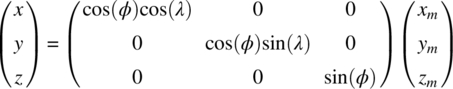
where the geographic polar coordinates (φ, λ) are computed as described in Section 20A.2 and the geomagnetic location of Px is determined as

The transformation from geographic‐to‐geomagnetic coordinates is accomplished by the appropriate interchange of the axes and polar angles.
20A.1 GEOGRAPHIC‐TO‐GEOMAGNETIC COORDINATE TRANSFORMATION
In this case the geographic coordinates (φ, λ) are known and the geomagnetic coordinates (Φ, Λ) are to be computed. Referring to the spherical triangle in Figure 20A.1 and applying the law of cosines16 results in the expression

that simplifies to
Using (20A.4) the geomagnetic latitude is determined as
The geomagnetic longitude is determined using the law of sines for spherical geometry that results in the expression
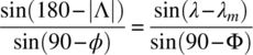
When simplified and rearranged (20A.6) results in the expression for sin(|Λ|)

Equation (20A.7) can be used to solve for Λ by using the trigonometric identity
Substituting (20A.4) to eliminate the dependence on Φ results in an involved expression and using (20A.7) results in a quadrant or sign ambiguity that needs to be resolved. A more satisfying approach is to use the law of cosines involving the longitude angle Λ expressed as

Upon simplifying (20A.9), solving for cos(|Λ|), then eliminating the dependence on sin(Φ) by substituting (20A.4), and performing some additional simplifications results in the desired expression

Equations (20A.7) and (20A.10) are now used to compute the magnetic longitude using the atan2(y, x) function with the result

The dependence on Φ in (20A.11) is eliminated by the formation of the ratio sin(|Λ|)/cos(|Λ|) inherent in the atan2( ) function. The advantage in using the atan2( ) function is that the angles are computed in the range 0 to ±180°17 so that angles 0 ≤ Λ ≤ 180° correspond to east longitudes or 0 ≥ Λ ≥ −180° correspond to west longitudes.
20A.2 GEOMAGNETIC‐TO‐GEOGRAPHIC COORDINATE TRANSFORMATION
In this case the geomagnetic coordinates (Φ, Λ) are known and the geomagnetic coordinates (φ, λ) are to be computed. The analysis follows similar lines of reasoning as in the preceding section so only the principal equations are given. Using the law of cosines the geographic latitude is evaluated as
Using the law of sines sin(λ − λm) is evaluated as

Applying the law of cosines cos(λ − λm) is evaluated, after substitutions and simplifications similar to those described in arriving at (20A.10), as

Using (20A.13) and (20A.14) and the ![]() function, the geographic longitude is computed as
function, the geographic longitude is computed as
ACRONYMS
- a.m.
- Before noon
- ARDC
- Air Research and Development Command
- ARQ
- Automatic repeat request
- AS
- Antiscintillation
- AWGN
- Additive white Gaussian noise
- BCI
- Bit count integrity
- BPSK
- Binary phase shift keying
- DCBPSK
- Differentially coherent BPSK
- DCMPSK
- Differentially coherent multiphase shift keying
- DCQPSK
- Differentially coherent QPSK
- DEBPSK
- Differentially encoded BPSK
- EAM
- Emergency action message
- EGD
- Equal gain diversity
- FEC
- Forward error correction (coding)
- FFRL
- Fast fading Rayleigh limit
- GEO
- Geostationary orbit
- GSO
- Geosynchronous orbit
- HEO
- Highly elliptical orbit
- INTELSATa
- International telecommunications satellite
- ISI
- Intersymbol interference
- LEO
- Low Earth orbit
- LOS
- Line of sight
- MAC
- Medium access control (protocol)
- NC M‐ary FSK
- Noncoherent M‐ary frequency shift keying or NCMFSK (detection)
- MFP
- Magnetic field plane
- MIMO
- Multiple‐in multiple‐out (antenna)
- MRCD
- Maximum ratio combining diversity
- NC
- Noncoherent (detection)
- NCMFSK
- Noncoherent multifrequency shift keying or NC M‐ary FSK (detection)
- OGO
- Orbiting geophysical observatory
- p.m.
- After noon
- PPSD
- Phase power spectral density
- QPSK
- Quadrature phase shift keying
- RF
- Radio frequency
- SD
- Selection diversity
- SFRL
- Slow fading Rayleigh limit
- TAB
- Time after blast
- TACSAT
- Tactical satellite (UHF)
- TEC or NT
- Total electron content (electrons/m2)
- UHF
- Ultra‐high frequency
Note: RAKE is not an acronym; it is the name applied to a wide bandwidth multipath correlator.
a INTELSAT© Corporation is a communications satellite services provider.
PROBLEMS
- Consider the inverse Fourier transform of the filter function H(u) expressed in the indefinite formThe general solution, expressed in terms of the parameters a, b, and c and the Fresnel integrals, is [30]
 Considering the definite integral with lower and upper integration limits −πW and πW and noting that
 ,
,  , and
, and  :
:
- Derive the expression for the magnitude of h(t) and express the result in terms of the Fresnel integrals and the parameters ρ, t, To, ϕ, and W.
- Derive the expression for the phase of h(t) and express the result in terms of the Fresnel integrals and the parameters ρ, t, To, ϕ, and W.
- Using the spherical triangle in Figure 20A.1 write the expression for the law of cosines for determining the geographic latitude φ and write the simplifying equations leading to (20A.12).
- Using the spherical triangle in Figure 20A.1 write the expression for the law of sines for determining sin(λ − λm) and write the simplifying equations leading to (20A.13).
- Using the spherical triangle in Figure 20A.1 write the expression for the law of cosines for determining cos(λ − λm) and write the simplifying equations and manipulations leading to (20A.14).
Hint: Use the trigonometric identity  .
.
REFERENCES
- 1. M.G. Morgan, Guest Editor, “The Nature of the Ionosphere – An IGY Objective,” Special Issue on the International Geophysical Year Objectives, Proceedings of the IRE, Vol. 47, No. 2, pp. 129–351, February 1959.
- 2. S. Chapman, “The Absorption and Disassociative Ionizing Effect of Monochromatic Radiation in an Atmosphere of a Rotating Earth,” Proceeding of the Physical Society, Vol. 43, pp. 26–45, 1931. Proceeding of the Physical Society, London, England, 1931.
- 3. K. Davies, Ionospheric Radio Propagation, National Bureau of Standards Monograph, No. 80, United States Department of Commerce, National Bureau of Standards, Washington, DC, April 1, 1965.
- 4. R.A. Minzner, K.S.W. Champion, H.L. Pond, The ARDC Model Atmosphere, AFCRC‐TR‐59‐267, Air Force Surveys in Geophysics, No. 115, Photochemistry Laboratory, Geophysics Research Directorate, Air Force Cambridge Research Center, Air Research and Development Command, Air Force Surveys in Geophysics, Bedford, MA, August 1959.
- 5. R.S. Berkowitz, Editor, Modern Radar, Analysis, Evaluation and System Design, Part V, Chapter 1, G.H. Millman, “Atmospheric Effects on Radio Wave Propagation,” John Wiley & Sons, Inc., New York, 1966.
- 6. R.S. Berkowitz, Editor, Modern Radar, Analysis, Evaluation and System Design, Part V, Chapter 1, G.H. Millman, “Atmospheric Effects on Radio Wave Propagation,” John Wiley & Sons, Inc., New York, 1966, p. 321, Tables 1‐2 and 1‐3.
- 7. R.L. Bogusch, “Ionospheric Scintillation Effects on Satellite Communications,” Interim Technical Note MRC‐N‐139, Mission Research Corporation, Santa Barbara, CA, June 1974.
- 8. J.P. McClure, W.E. Hanson, “A Catalog of Ionospheric F‐Region Irregularity Behavior Based on Ogo 6 Retarding Potential Analyzer Data,” Journal of Geophysical Research, Vol. 78, No. 31, pp. 7431–7440, November 1973.
- 9. A.L. Johnson, “The Effects of Ionospheric Scintillation on Satellite Communications,” Air and Space University Review, Vol. 24, No. 6, pp. 26–31, November–December 1973, U.S. Air Force, Maxwell AFB, AL.
- 10. M.R. Paulson, R.U.F. Hopkins, “Effects of Equatorial Scintillation Fading on SATCOM Signals,” NELC/TR 1875, Naval Electronics Laboratory Center, San Diego, CA, May 8, 1973.
- 11. L.A. Wittwer, “Satellite Communications in a Scintillated Environment,” Air Force Weapons Laboratory, Report AFWL‐TR‐75‐240, January 1976. Also available from NTIS AD/A‐021‐091.
- 12. R.R. Taur, “Ionospheric Scintillation at 4 and 6 GHz,” COMSAT Technical Review, Vol. 3, No. 1, pp. 145–163, Spring 1973.
- 13. L.A. Wittwer, “Satellite Communications in a Scintillated Environment,” Air Force Weapons Laboratory, Report AFWL‐TR‐75‐240, p. 39, January 1976.
- 14. C.M. Rush, “An Ionospheric Observation Network for Use in Short‐Term Propagation Predictions,” Telecommunications Journal, Vol. 43, pp. 544–548, August 1976.
- 15. G.N. Taylor, “The Seasonal Anomaly in Electron Content,” J. Frihagen, Editor, Proceedings of NATO Advanced Studies Institute, pp. 543–548, Ohrid, Bulgaria, 1965.
- 16. R.S. Berkowitz, Editor, Modern Radar, Analysis, Evaluation and System Design, Part V, Chapter 1, G.H. Millman, “Atmospheric Effects on Radio Wave Propagation,” John Wiley & Sons, Inc., New York, 1966, p. 322, Table 1‐4.
- 17. R.W. Middlestead, R.E. LeLevier, M.D. Smith, “Satellite Crosslink Communications Vulnerability in a Nuclear Environment,” IEEE Journal on Selected Area in Communications, Vol. SAC‐5, No. 2, pp. 138–145, February 1987.
- 18. J.A. Stratton, Electromagnetic Theory, p. 327, McGraw Hill Book Company, Inc., New York, 1941.
- 19. J.A. Ratcliffe, The Magneto‐Ionic Theory and Its Application to the Ionosphere, Cambridge University Press, New York, 1959.
- 20. K.G. Budden, Radio Waves in the Ionosphere, Cambridge University Press, New York, 1959.
- 21. K.G. Budden, The Wave‐Guide Mode Theory of Wave Propagation, Logos Press/Prentice‐Hall, London/Englewood Cliffs, NJ, 1961.
- 22. J.M. Kelso, Radio Ray Propagation in the Ionosphere, McGraw‐Hill Co. Inc., New York, 1964.
- 23. D.R. McDaniel, “Proceedings of the DNA/LASL High‐Altitude Nuclear Weapons Effects Summer Study (U), Vol. II—Working Group Reports (U),” DNA 4736P‐3, SRI International, Menlo Park, CA, November 1, 1978.
- 24. L.A. Wittwer, “Radio Wave Propagation in Structured Ionization for Satellite Applications,” Report DNA 5304D, Defense Nuclear Agency, Washington, DC, December 1979.
- 25. RDA Staff, “Nuclear Effects Handbook for Satellite Communications (U),” Research and Development Associates (RDA), pp. 2–23, Marina Del Rey, CA, May 1986.
- 26. RDA Staff, “Nuclear Effects Handbook for Satellite Communications (U),” Research and Development Associates (RDA), pp. 2–26, Marina Del Rey, CA, May 1986.
- 27. RDA Staff, “Nuclear Effects Handbook for Satellite Communications (U),” Research and Development Associates, pp. 2–21, Marina Del Rey, CA, May 1986.
- 28. RDA Staff, “Nuclear Effects Handbook for Satellite Communications (U),” Research and Development Associates, pp. 2–24, 25, Marina Del Rey, CA, May 1986.
- 29. W.S. Knapp, K. Schwartz, “Aids for the Study of Electromagnetic Blackout(U),” Report, DNA 3499H, General Electric—TEMPO, Santa Barbara, CA, February 1975.
- 30. M. Abramowitz, I.A. Stegun, Handbook of Mathematical Functions with Formulas, Graphs, and Mathematical Tables, Applied Mathematics Series, No. 55, p. 304, U.S. Department of Commerce, Washington, DC, June 1964.
- 31. L.A. Wittwer, “The Propagation of Satellite Signals Through a Turbulent Media,” Air Force Weapons Laboratory, Report AFWL‐TR‐77‐183, Kirkland Air Force Base, NM, January 1978.
- 32. D.L. Knepp, “Multiple Phase‐Screen Calculation of the Temporal Behavior of Stochastic Waves,” Proceeding of the IEEE, Vol. 71, No. 6, pp. 722–737, June 1983.
- 33. D.L. Knepp, “Multiple Phase‐Screen Propagation Analysis for Defense Satellite Communications Systems,” Report DNA‐4424T, Defense Nuclear Agency, Washington, DC, September 1977.
- 34. R.L. Bogusch, F.W. Guigliano, “Nuclear Survivability Criteria for Satellite Links(U),” Final Report, AFWL‐TR‐82‐18, Mission Research Corporation, Santa Barbara, CA, October 1982.
- 35. M. Torlak, T.M. Duman, “MIMO Communication Theory, Algorithms, and Prototyping,” Proceedings of the 20th Signal Processing and Communications Applications Conference (SIU), Mugla, April 18–20, 2012.
- 36. S. Choi, Y.C. Ko, E.J. Powers, “Optimization of Switched MIMO Systems Over Rayleigh Fading Channels,” IEEE Transactions on Vehicular Technology, Vol. 56, No. 1, pp. 103–114, January 2007.
- 37. M. Chiani, M.Z. Win, S. Hyundong, “MIMO Networks: The Effects of Interference,” IEEE Transactions on Information Theory, Vol. 56, No. 1, pp. 336–349, January 2010.
- 38. L. Hanzo, M. El‐Hajjar, O. Alamri, “Near Capacity Wireless Transceivers and Cooperative Communications in the MIMO Era: Evolution of Standards, Waveform Design, and Future Perspectives,” Proceeding of the IEEE, Vol. 99, No. 8, pp. 1343–1385, August 2011.
- 39. R.W. Middlestead, “Performance of DC‐PSK Modulation with Concatenated Coding in a Nuclear Environment,” Air Force Weapons Laboratory, AFWL‐TR‐81‐191, Rockwell International, Newport Beach, CA, February 1982.
- 40. A.J. Viterbi, I.M. Jacobs, “Advances in Coding and Modulation for Noncoherent Channels Affected by Fading, Partial Band, and Multiple‐Access Interference,” A.J. Viterbi, Editor, Advances in Communication Systems, Vol. 4, pp. 279–308, Academic Press, New York, 1975.
- 41. J.P. Odenwalder, “Error Control Coding Handbook,” Prepared Under USAF Contract No. F44620‐76‐C‐0056, Final Report, pp. 24–28, Linkabit Corporation, San Diego, CA, July 15, 1976.
- 42. O.W. Eshbach, Handbook of Engineering Fundamentals, Wiley Engineering Handbook Series, John Wiley & Sons, Inc., New York, 1952.