
1
MATHEMATICAL BACKGROUND AND ANALYSIS TECHNIQUES
1.1 INTRODUCTION
This introductory chapter focuses on various mathematical techniques and solutions to practical problems encountered in many of the following chapters. The discussions are divided into three distinct topics: deterministic signal analysis involving linear systems and channels; statistical analysis involving probabilities, random variables, and random processes; miscellaneous topics involving windowing functions, mathematical solutions to commonly encountered problems, and tables of commonly used mathematical functions. It is desired that this introductory material will provide the foundation for modeling and finding practical design solutions to communication system performance specifications. Although this chapter contains a wealth of information regarding a variety of topics, the contents may be viewed as reference material for specific topics as they are encountered in the subsequent chapters.
This introductory section describes the commonly used waveform modulations characterized as amplitude modulation (AM), phase modulation (PM), and frequency modulation (FM) waveforms. These modulations result in the transmission of the carrier‐ and data‐modulated subcarriers that are accompanied by negative frequency images. These techniques are compared to the more efficient suppressed carrier modulation that possesses attributes of the AM, PM, and FM modulations. This introduction concludes with a discussion of real and analytic signals, the Hilbert transform, and demodulator heterodyning, or frequency mixing, to baseband.
Sections 1.2–1.4, deterministic signal analysis, transform in the context of a uniformly weighted pulse f(t) and its spectrum F(f) and the duality between ideal time and frequency sampling that forms the basis of Shannon’s sampling theorem [1]. This section also discusses the discrete Fourier transform (DFT), the fast Fourier transform (FFT), the pipeline implementation of the FFT, and applications involving waveform detection, interpolation, and power spectrum estimation. The concept of paired echoes is discussed and used to analyze the signal distortion resulting from a deterministic band‐limited channel with amplitude and phase distortion. These sections conclude on the subject of autocorrelation and cross‐correlation of real and complex deterministic functions; the corresponding covariance functions are also examined.
Sections 1.5–1.10, statistical analysis, introduce the concept of random variables and various probability density functions (pdf) and cumulative distribution functions (cdf) for continuous and discrete random variables. Stochastic processes are then defined and the properties of ergodic and stationary random processes are examined. The characteristic function is defined and examples, based on the summation of several underlying random variables, exhibit the trend in the limiting behavior of the pdf and cdf functions toward the normal distribution; thereby demonstrating the central limit theorem. Statistical analysis using distribution‐free or nonparametric techniques is introduced with a focus on order statistics. The random process involving narrowband white Gaussian noise is characterized in terms of the noise spectral density at the input and output of an optimum detection filter. This is followed by the derivation of the matched filter and the equivalence between the matched filter and a correlation detector is also established. The next subject discussed involves the likelihood ratio and log‐likelihood ratio as they pertain to optimum signal detection. These topics are generalized and expanded in Chapter 3 and form the basis for the optimum detection of the modulated waveforms discussed in Chapters 4–9. Section 1.9 introduces the subject of parameter estimation which is revisited in Chapters 11 and 12 in the context of waveform acquisition and adaptive systems. The final topic in this section involves a discussion of modem configurations and the important topic of automatic repeat request (ARQ) to improve the reliability of message reception.
Sections 1.11–1.14, miscellaneous topics, include a characterization of several window functions that are used to improve the performance the FFT, decimation filtering, and signal parameter estimation. Section 1.12 provides an introductory discussion of matrix and vector operations. In Section 1.13 several mathematical procedures and formulas are discussed that are useful in system analysis and simulation programming. These formulas involve prime factorization of an integer and determination of the greatest common factor (GCF) and least common multiple (LCM) of two integers, Newton’s approximation method for finding the roots of a transcendental function, and the definition of the standard deviation of a sampled population. This chapter concludes with a list of frequently used mathematical formulas involving infinite and finite summations, the binomial expansion theorem, trigonometric identities, differentiation and integration rules, inequalities, and other miscellaneous relationships.
Many of the examples and case studies in the following chapters involve systems operating in a specific frequency band that is dictated by a number of factors, including, the system objectives and requirements, the communication range equation, the channel characteristics, and the resulting link budget. The system objectives and requirements often dictate the frequency band that, in turn, identifies the channel characteristics. Table 1.1 identifies the frequency band designations with the corresponding range of frequencies. The designations low frequency (LF), medium frequency (MF), and high frequency (HF) refer to low, medium, and high frequencies and the prefixes E, V, U, and S correspond to extremely, vary, ultra, and super.
TABLE 1.1 Frequency Band Designations
| Designation | Frequency | Letter Designation | Frequency (GHz) |
| ELF | 3–30 Hz | L | 1–2 |
| SLF | 30–300 Hz | S | 2–4 |
| ULF | 0.3–3 kHz | C | 4–8 |
| VLF | 3–30 kHz | X | 8–12 |
| LF | 30–300 kHz | Ku | 12–18 |
| MF | 0.3–3 MHz | K | 18–27 |
| HF | 3–30 MHz | Ka | 27–40 |
| VHF | 30–300 MHz | V | 40–75 |
| UHF | 0.3–3 GHz | W | 75–110 |
| SHF | 3–30 GHz | mm (millimeter) | 110–300 |
| EHF | 30–300 GHz |
1.1.1 Waveform Modulation Descriptions
This section characterizes signal waveforms comprised of baseband information modulated on an arbitrary carrier frequency, denoted as fc Hz. The baseband information is characterized as having a lowpass bandwidth of B Hz and, in typical applications, fc >> B. In many communication system applications, the carrier frequency facilitates the transmission between the transmitter and receiver terminals and can be removed without effecting the information. When the carrier frequency is removed from the received signal the signal processing sampling requirements are dependent only on the bandwidth B.
The signal modulations described in Sections 1.1.1.1 through 1.1.1.4 are amplitude, phase, frequency, and suppressed carrier modulations. The amplitude, phase, and frequency modulations are often applied to the transmission of analog information; however, they are also used in various applications involving digital data transmission. For example, these modulations, to varying degrees, are the underlying waveforms used in the U.S. Air Force Satellite Control Network (AFSCN) involving satellite uplink and downlink control, status, and ranging.
In describing the demodulator processing of the received waveforms, the information, following removal of the carrier frequency, is associated with in‐phase and quadphase (I/Q) baseband channels or rails. Although these I/Q channels are described as containing quadrature real signals, they are characterized as complex signals with real and imaginary parts. This complex signal description is referred to as complex envelope or analytic signal representations and is discussed in Section 1.1.1.5. Suppressed carrier modulation and the analytic signal representation emphasize quadrature data modulation that leads to a discussion of the Hilbert transform in Section 1.1.1.6. Section 1.1.1.7 discusses conventional heterodyning of the received signal to baseband followed by data demodulation.
1.1.1.1 Amplitude Modulation
Conventional amplitude modulation (AM) is characterized as
where A is the peak carrier voltage, ![]() is the modulation index, m(t) is the information modulation function, ωm is the modulation angular frequency, and ωc is the AM carrier angular frequency. Upon multiplying (1.1) through by sin(ωct) and applying elementary trigonometric identities, the AM‐modulated signal is expressed as
is the modulation index, m(t) is the information modulation function, ωm is the modulation angular frequency, and ωc is the AM carrier angular frequency. Upon multiplying (1.1) through by sin(ωct) and applying elementary trigonometric identities, the AM‐modulated signal is expressed as

Therefore, s(t) represents the conventional double sideband (DSB) AM waveform with the upper and lower sidebands at ![]() equally spaced about the carrier at ωc. With the information modulation function m(t) normalized to unit power, the power in each sideband is mIPS/4 where PS is the power in the carrier frequency fc.
equally spaced about the carrier at ωc. With the information modulation function m(t) normalized to unit power, the power in each sideband is mIPS/4 where PS is the power in the carrier frequency fc.
1.1.1.2 Phase Modulation
Conventional phase modulation (PM) is characterized as
where A is the peak carrier voltage, ωc is the carrier angular frequency, and φ(t) is an arbitrary phase modulation function containing the information. The commonly used phase function is expressed as
where ϕ is the peak phase deviation. Substituting (1.4) into (1.3), the phase‐modulated signal is expressed as
and, upon applying elementary trigonometric identities, (1.5) yields
The trigonometric functions involving sinusoidal arguments can be expanded in terms of Bessel functions [2] and (1.6) simplifies to

Equation (1.7) is characterized by the carrier frequency with peak amplitude AJ0(ϕ) and upper and lower sideband pairs at ![]() with peak amplitudes AJn(ϕ). For small arguments the Bessel functions reduce to the approximations
with peak amplitudes AJn(ϕ). For small arguments the Bessel functions reduce to the approximations ![]() with
with ![]() and (1.7) reduces to
and (1.7) reduces to

Under these small argument approximations, the similarities between (1.8) and (1.2) are apparent.
1.1.1.3 Frequency Modulation
The frequency‐modulated (FM) waveform is described as

where A is the peak carrier voltage, ωc is the carrier angular frequency, Δf is the peak frequency deviation of the modulation frequency fm, and ωm is the modulation angular frequency. The ratio Δf/fm is the frequency modulation index. Noting the similarities between (1.9) and (1.5), the expression for the frequency‐modulated waveform is expressed, in terms of the Bessel functions, as

with the corresponding small argument approximation for the Bessel function expressed as

The similarities between (1.11), (1.8), and (1.2) are apparent.
1.1.1.4 Suppressed Carrier Modulation
A commonly used form of modulation is suppressed carrier modulation expressed as
In this case, when the carrier is mixed to baseband, information modulation function m(t) does not have a direct current (DC) spectral component involving δ(ω). So, upon multiplication by the carrier, there is no residual carrier component ωc in the received baseband signal. Because the carrier is suppressed it is not available at the receiver/demodulator to provide a coherent reference, so special considerations must be given to the carrier recovery and subsequent data demodulation. Suppressed carrier‐modulated waveforms are efficient, in that, all of the transmitted power is devoted to the information. Suppressed carrier modulation and the various methods of carrier recovery are the central focus of the digital communication waveforms discussed in the following chapters.
1.1.1.5 Real and Analytic Signals
The earlier modulation waveforms are described mathematically as real waveforms that can be transmitted over real or physical channels. The general description of the suppressed carrier waveform, described in (1.12), can be expressed in terms of in‐phase and quadrature modulation functions mc(t) and ms(t) as
The quadrature modulation functions are expressed as
and
With PM the data {dc, ds} may be contained in a phase function φd(t), m(t) is a unit energy symbol shaping function that provides for spectral control relative to the commonly used rect(t/T) function, and A represents the peak carrier voltage on each rail. With quadrature modulations, unique symbol shaping functions, mc(t) and ms(t), may be applied to each rail; for example, unbalanced quadrature modulations involve different data rates on each quadrature rail. With quadrature amplitude modulation (QAM) the data is described in terms of the multilevel quadrature amplitudes {αc, αs} that are used in place of {dc, ds} in (1.14) and (1.15).
Equation (1.13) can also be expressed in terms of the real part of a complex function as
where
The function ![]() is referred to as the complex envelope or analytic representation of the baseband signal and plays a fundamental role in the data demodulation, in that, it contains all of the information necessary to optimally recover the transmitted information. Equation (1.17) applies to receivers that use linear frequency translation to baseband. Linear frequency translation is typical of heterodyne receivers using intermediate frequency (IF) stages. This is a significant result because the system performance can be evaluated using the analytic signal without regard to the carrier frequency [3]; this is particularly important in computer performance simulations.
is referred to as the complex envelope or analytic representation of the baseband signal and plays a fundamental role in the data demodulation, in that, it contains all of the information necessary to optimally recover the transmitted information. Equation (1.17) applies to receivers that use linear frequency translation to baseband. Linear frequency translation is typical of heterodyne receivers using intermediate frequency (IF) stages. This is a significant result because the system performance can be evaluated using the analytic signal without regard to the carrier frequency [3]; this is particularly important in computer performance simulations.
Evaluation of the real part of the signal expressed in (1.16) is performed using the complex identity No. 4 in Section 1.14.6 with the result
A note of caution is in order, in that, the received signal power based on the analytic signal is twice that of the power in the carrier. This results because the analytic signal does not account for the factor of 1/2 when mixing or heterodyning with a locally generated carrier frequency and is directly related the factor of 1/2 in (1.18). The signal descriptions expressed in (1.12) through (1.18) are used to describe the narrowband signal characteristics used throughout much of this book.
1.1.1.6 Hilbert Transform and Analytic Signals
The Hilbert transform of the real s(t) is defined as

The second expression in (1.19) represents the convolution of s(t) with a filter with impulse response ![]() where h(t) represents the response to a Hilbert filter with frequency response H(ω) characterized as
where h(t) represents the response to a Hilbert filter with frequency response H(ω) characterized as

The Hilbert transform of s(t) results in a spectrum that is zero for all negative frequencies with positive frequencies representing a complex spectrum associated with the real and imaginary parts of an analytic function. Applying (1.20) to the signal spectrum ![]() results in the spectrum of the Hilbert transformed signal
results in the spectrum of the Hilbert transformed signal

Applying (1.21) to the spectrum S(ω) of (1.12) or (1.13), the bandwidth B of m(t) must satisfy the condition B << fc. In this case, the inverse Fourier transform of the spectrum ![]() yields the Hilbert filter output
yields the Hilbert filter output ![]() given by
given by

where TH[s(t)] represents the Hilbert transform of s(t).
The function ![]() expressed by (1.22) is orthogonal to s(t) and, if the carrier frequency were removed following the Hilbert transform, the result would be identical to the imaginary part of the analytic signal expressed by (1.17). The processing is depicted in Figure 1.1.
expressed by (1.22) is orthogonal to s(t) and, if the carrier frequency were removed following the Hilbert transform, the result would be identical to the imaginary part of the analytic signal expressed by (1.17). The processing is depicted in Figure 1.1.

FIGURE 1.1 Hilbert transform of carrier‐modulated signal s(t)  .
.
1.1.1.7 Conventional and Complex Heterodyning
Conventional heterodyning is depicted in Figure 1.2. The zonal filters are ideal low‐pass filters with frequency response given by
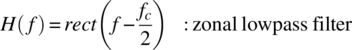

FIGURE 1.2 Heterodyning of carrier‐modulated signal s(t)  .
.
These filters remove the 2ωc term that results from the mixing operation and, for s(t) as expressed by (1.13), the quadrature outputs are given by
and
With ideal phase tracking the phase term ϕ(t) is zero resulting in the quadrature modulation functions mc(t) and ms(t) in the respective low‐pass channels.
1.2 THE FOURIER TRANSFORM AND FOURIER SERIES
The Fourier transform is so ubiquitous in the technical literature [4–6], and its application are so widely used that it seems unnecessary to dwell at any length on the subject. However, a brief description is in order to aid in the understanding of the parameters used in the applications discussed in the following chapters.
The Fourier transform F(f) of f(t) is defined over the interval ![]() and, if f(t) is absolutely integrable, that is, if
and, if f(t) is absolutely integrable, that is, if

then F(f) exists, furthermore, the inverse Fourier transform of F(f) results in f(t). In most applications1 of practical interest, f(t) satisfies (1.26) leading to the Fourier transform pair ![]() defined as
defined as

In general, f(t) is real and the Fourier transform F(f) is complex and Parseval’s theorem relates the signal energy in the time and frequency domains as

The Fourier series representation of a periodic function is closely related to the Fourier transform; however, it is based on orthogonal expansions of sinusoidal functions at discrete frequencies. For example, if the function of interest is periodic, such that, f(t) = f(t – iTo) with period To and is finite and single valued over the period, then f(t) can be represented by the Fourier series

where ωo = 2π/To and Cn is the n‐th Fourier coefficient given by

Equation (1.29) is an interesting relationship, in that, f(t) can be described over the time interval To by an infinite set of frequency‐domain coefficient Cn; however, because f(t) is contiguously replicated over all time, that is, it is periodic, the spectrum of f(t) is completely defined by the coefficients Cn. Unlike the Fourier transform, the spectrum of (1.29) is not continuous in frequency but is zero except at discrete frequencies occurring at multiples of nωo. This is seen by taking the Fourier transform of (1.29) and, using (1.27), the result is expressed as

where ![]() is the Fourier Transform2 of
is the Fourier Transform2 of ![]() . Equation (1.31) is applied in Chapter 2 in the discussion of sampling theory and in Chapter 11 in the context of signal acquisition.
. Equation (1.31) is applied in Chapter 2 in the discussion of sampling theory and in Chapter 11 in the context of signal acquisition.
Alternate forms of (1.29) that emphasize the series expansion in terms of harmonics of trigonometric functions are given in (1.32) and (1.33) when f(t) is a real‐valued function. This is important because when f(t) is real the complex coefficients Cn and C−n form a complex conjugate pair such that ![]() which simplifies the evaluation of f(t). For example, using the complex notations
which simplifies the evaluation of f(t). For example, using the complex notations ![]() and
and ![]() , the function f(t) is evaluated as
, the function f(t) is evaluated as

this simplifies to

where ![]() and
and ![]() .
.
An important consideration in spectrum analysis is the determination of signal spectrums involving random data sequences, referred to as stochastic processes [8]. A stochastic process does not have a unique spectrum; however, the power spectral density (PSD) is defined as the Fourier transform of the autocorrelation response. Oppenheim and Schafer [9] discuss methods of estimating the PSD of a real finite‐length (N) sampled sequence by averaging periodograms, defined as
where F(ω) is the Fourier transform of the sampled sequence. This method is accredited to Bartlett [10] and is used in the evaluation of the PSD in the following chapters. For a fixed length (L) of random data, the number of periodograms (K) that can be averaged is K = L/N. As K increases the variance of the spectral estimate approaches zero and as N increases the resolution of the spectrum increases, so there is a trade‐off between the selection of K and N. To resolve narrowband spectral features that occur, for example, with nonlinear frequency shift keying (FSK)‐modulated waveforms, it is important to use large values of N. Fortunately, many of the spectrum analyses presented in the following chapters are not constrained by L so K and N are chosen to provide a low estimation bias, that is, low variance, and high spectral resolution. Windowing3 the periodograms will also reduce the estimation bias at the expense of decreasing the spectral resolution.
1.2.1 The Transform Pair rect(t/T) ⇔ Tsinc(fT)
The transform relationship rect(t/T) ⇔ Tsinc(fT) occurs so often that it deserves special consideration. For example, consider the following function:

where ωc, τ, and ϕ represent arbitrary angular frequency, delay, and phase parameters. The signal s(t) is depicted in Figure 1.3.

FIGURE 1.3 Pulse‐modulated carrier.
The Fourier transform of s(t) is evaluated as

Expressing the cosine function in terms of complex exponential functions and performing some simplifications results in the expression

Evaluation of the integrals in (1.37) appears so often that it is useful to generalize the solutions as follows:
Consider the integral

The general solution involves multiplying the last equality in (1.38) by the factors ![]() and
and ![]() , having a product of one, where
, having a product of one, where ![]() is the average of the integration limits. Distributing the second factor over the numerator of (1.38) and then simplifying yields the result
is the average of the integration limits. Distributing the second factor over the numerator of (1.38) and then simplifying yields the result

Applying (1.39) to (1.37) and simplifying gives the desired result
When ![]() , the positive and negative frequency spectrums do not influence one another and, in this case, the positive frequency spectrum is defined as
, the positive and negative frequency spectrums do not influence one another and, in this case, the positive frequency spectrum is defined as
On the other hand, when the carrier frequency and phase are zero, (1.40) simplifies to the baseband spectrum, evaluated as
Using (1.42), the baseband Fourier transform pair, corresponding to of (1.35) with fc = 0, is established as

and, with τ = 0,
1.2.2 The sinc(x) Function
The sinc(x) function is defined as
and is depicted in Figure 1.4. When x is expressed as the normalized frequency variable x = fT then (1.45), when scaled by T, is the frequency spectrum of the unit amplitude pulse rect(t/T) of duration T seconds such that t ≤ |T/2|. This function is symmetrical in x and the maximum value of the first sidelobe occurs at x = 1.431 with a level of 10log(sinc2(x)) = −13.26 dB; the peak sidelobe levels decrease in proportion to 1/|x|. The noise bandwidth of a filter function H(f) is defined as

where fo is the filter frequency corresponding to the maximum response. When a receiver filter is described as H(f) = sinc(fT) the receiver low‐pass noise bandwidth is evaluated as Bn = 1/T where T is the duration of the filter impulse response.

FIGURE 1.4 The sinc(x) function.
It is sometimes useful to evaluate the area of the sinc(x) function and, while there is no closed form solutions, the solution can be evaluated in terms of the sine‐integral Si(x)4 as

where the sine‐integral is defined as the integral of sin(λ)/λ. Equation (1.47) is shown in Figure 1.5. The limit of Si(πz) as |z| → ∞ is5 π sign(1,z)/2 so the corresponding limit of (1.47) is 0.5sgn(z).

FIGURE 1.5 Integral of sinc(x).
A useful parameter, often used as a benchmark for comparing spectral efficiencies, is the area under sinc2(x) as a function of x. The area is evaluated in terms of the sine‐integral as

Equation (1.48) is plotted in Figure 1.6 as a percent of the total area and it is seen that the spectral containment of 99% is in excess of 18 spectral sidelobes, that is, x = fT = 18. In the following chapters, spectral efficient waveforms are examined with 99% containment within 2 or 3 sidelobes, so the sinc(x) function does not represent a spectrally efficient waveform modulation.

FIGURE 1.6 Integral of sinc2(x) function.
1.2.3 The Fourier Transform Pair 
The evaluation of this Fourier transform pair is fundamental to Nyquist sampling theory and is demonstrated in Section 2.3 in the evaluation of discrete‐time sampling. In this case, the function f(t) is an infinite repetition of equally spaced delta functions δ(t) with intervals T seconds as expressed by

The challenge is to show that the Fourier transform of (1.49) is equal to an infinite repetition of equally spaced and weighted frequency domain delta functions expressed as

with weighting ωo and frequency intervals ![]() . Direct application of the Fourier transform to (1.49) leads to the spectrum
. Direct application of the Fourier transform to (1.49) leads to the spectrum ![]() but this does not demonstrate the equality in (1.50). Similarly, evaluation of the inverse Fourier transform of (1.50) results in the time‐domain expression
but this does not demonstrate the equality in (1.50). Similarly, evaluation of the inverse Fourier transform of (1.50) results in the time‐domain expression

So, by showing that ![]() , the transform pair between (1.49) and (1.50) will be established. Consider gN(t) to be a finite summation of terms in (1.51) given by
, the transform pair between (1.49) and (1.50) will be established. Consider gN(t) to be a finite summation of terms in (1.51) given by

The second equality in (1.52) can be shown using the finite series identity No. 12, Section 1.14.1. Equation (1.52) is referred to by Papoulis [7] as the Fourier‐series kernel and appears in a number of applications involving the Fourier transform.
The function gN(t) is plotted in Figure 1.7 for N = 8. The abscissa is time normalized by the pulse repetition interval ![]() such that,
such that, ![]() , and there are a total of
, and there are a total of ![]() peaks of which three are shown in the figure. Furthermore, there are eight time sidelobes between t/T = 0 and 0.5 with the first nulls from the peak value at t/T = 0 occurring at
peaks of which three are shown in the figure. Furthermore, there are eight time sidelobes between t/T = 0 and 0.5 with the first nulls from the peak value at t/T = 0 occurring at ![]() ; the peak values are
; the peak values are ![]() in this example.
in this example.

FIGURE 1.7 The Fourier‐series kernel gN(t) (N = 8).
The maximum values of ![]() , occurring at
, occurring at ![]() , are determined by applying L’Hospital’s rule to (1.52), which is rewritten as
, are determined by applying L’Hospital’s rule to (1.52), which is rewritten as

The approximation in (1.53) is obtained by noting that as N increases the rate of the sinusoidal variations in the numerator term increases with a frequency of ![]() Hz while the rate of sinusoidal variation in the denominator remains unchanged. Therefore, in the vicinity of
Hz while the rate of sinusoidal variation in the denominator remains unchanged. Therefore, in the vicinity of ![]() ,
, ![]() and (1.53) reduces to a sin(x)/x function with
and (1.53) reduces to a sin(x)/x function with ![]() and a peak amplitude (2N + 1). The proof of the transform pair is completed by showing that f(t) = g(t). Referring to (1.51) g(t) is expressed as
and a peak amplitude (2N + 1). The proof of the transform pair is completed by showing that f(t) = g(t). Referring to (1.51) g(t) is expressed as
From (1.53) as N approaches infinity the sin(x)/x sidelobe nulls converge to t/T = n, the peak values become infinite, and the corresponding area over the interval |t/T| = n ± 1/2 approaches unity. Therefore, g(t) resembles a periodic series of delta functions resulting in the equality

thus completing the proof that (1.49) and (1.50) correspond to a Fourier transform pair. Papoulis (Reference 7, pp. 50–52) provides a more eloquent proof that the limiting form of gN(t) is indeed an infinite sequence of delta functions.
1.2.4 The Discrete Fourier Transform
The DFT pair relating the discrete‐time function f(mΔt) ≡ f(m) and discrete‐frequency function F(nΔf) ≡ F(n) is denoted as ![]() where
where

With the DFT the number of time and frequency samples can be chosen independently. This is advantageous when preparing presentation material or examining fine spectral or temporal details, as might be useful when debugging simulation programs, by the independent selection of the integers m and n.
1.2.5 The Fast Fourier Transform
As discussed in the preceding section, the DFT pair, relating the discrete‐time function f(mΔt) ≡ f(m) and the discrete‐frequency function F(nΔf) ≡ F(n), is denoted as ![]() where f(m) and F(n) are characterized by the expressions for the DFT. The FFT [11–17], is a special case corresponding to m and n being equal to N as described in the remainder of this section. In these relationships N is the number of time samples and is defined as the power of a fixed radix‐r FFT or as the powers of a mixed radix‐rj FFT.6 The fixed radix‐2 FFT, with r = 2 and N = 2i, results in the most processing efficient implementation.
where f(m) and F(n) are characterized by the expressions for the DFT. The FFT [11–17], is a special case corresponding to m and n being equal to N as described in the remainder of this section. In these relationships N is the number of time samples and is defined as the power of a fixed radix‐r FFT or as the powers of a mixed radix‐rj FFT.6 The fixed radix‐2 FFT, with r = 2 and N = 2i, results in the most processing efficient implementation.
Defining the time window of the FFT as Tw results in an implicit periodicity of f(t) such that f(t) = f(t ± kTw) and Δt = Tw/N. The sampling frequency is defined as ![]() and, based on Shannon’s sampling theorem, the periodicity does not pose a practical problem as long as the signal bandwidth is completely contained in the interval |B| ≤ fs/2 = N/(2Tw). Since the FFT results in an equal number of time and frequency domain samples, that is, Δf = fs/N and Δt = Tw/N, it follows that ΔfΔt = fs Tw/N2 = 1/N. Normalizing the expression of the time function, f(m), in (1.56), that is, multiplying the inverse DFT (IDFT) by Δt requires dividing the expression for F(n) by Δt. Upon substituting these results into (1.56), the FFT transform pairs become
and, based on Shannon’s sampling theorem, the periodicity does not pose a practical problem as long as the signal bandwidth is completely contained in the interval |B| ≤ fs/2 = N/(2Tw). Since the FFT results in an equal number of time and frequency domain samples, that is, Δf = fs/N and Δt = Tw/N, it follows that ΔfΔt = fs Tw/N2 = 1/N. Normalizing the expression of the time function, f(m), in (1.56), that is, multiplying the inverse DFT (IDFT) by Δt requires dividing the expression for F(n) by Δt. Upon substituting these results into (1.56), the FFT transform pairs become

The time and frequency domain sampling characteristics of the FFT are shown in Figure 1.8. This depiction focuses on a communication system example, in that, the time samples over the FFT window interval Tw are subdivided into Nsym symbol intervals of duration T seconds with Ns samples/symbol.

FIGURE 1.8 FFT time and frequency domain sampling.
Typically the bandwidth of the modulated waveform is taken to be the reciprocal of the symbol duration, that is, 1/T Hz; however, the receiver bandwidth required for low symbol distortion is typically several times greater than 1/T depending upon the type of modulation. Referring to Figure 1.8 the sampling frequency is fs = 1/Δt, the sampling interval is Δt = T/Ns, the size of the FFT is Nfft = NsNsym, and the frequency sampling increment is Δf = fs/Nfft. Upon using these relationships, the frequency resolution, or frequency samples per symbol bandwidth B = 1/T, is found to be
and the number of spectral sidelobes7 or symbol bandwidths over the sampling frequency range is
Therefore, to increase the resolution of the sampled signal spectrum, the number of symbols must be increased and this is comparable to increasing Tw. On the other hand, to increase the number of signal sidelobes contained in the frequency spectrum the number of samples per symbol must be increased and this is comparable to decreasing Δt. Both of these conditions require increasing the size (N) of the FFT. However, for a given size, the FFT does not allow independent selection of the frequency and time resolution as determined, respectively, by (1.58) and (1.59). This can be accomplished by using the DFT as discussed in Section 1.2.4. Since the spectrum samples in the range 0 ≤ f < fs/2 represent the positive frequency signal spectrum and those over the range fs/2 ≤ f < fs represent the negative frequency signal spectrum, the range of signal sidelobes of interest is ±fs/(2B) = ±Ns/2. As a practical matter, if the signal carrier frequency is not zero then the sampling frequency must be increased to maintain the signal sidelobes aliasing criterion. The sampling frequency selection is discussed in Chapter 11 in the context of signal acquisition when the received signal frequency is estimated based on locally known conditions.
The following implementation of the FFT is based on the Cooley and Tukey [18] decimation‐in‐time algorithm as described by Brigham and Morrow [19] and Brigham [20]. Although (1.57) characterizes the FFT transform pairs, the real innovation leading to the fast transformation is realized by the efficient algorithms used to execute the transformation. Considering the radix‐2 FFT with N = 2n, this involves defining the constant
and recognizing that

Equation (1.61) can be expressed in matrix form, using N = 4 for simplicity, as

Recognizing that W0 = 1 and the exponent nm is modulo(N), upon factoring the matrix in (1.62) into the product of two submatrices (in general the product of log2N submatrices) leads to the implementation involving the minimum number of computations expressed as

The simplifications result in the outputs F(2) and F(1) being scrambled and the unscrambling to the natural‐number ordering simply involves reversing the binary number equivalents, that is, with F′(1) = F(2) and F′(2) = F (1); therefore, the unscrambling is accomplished as F(1) = F (01) = F′(2) = F′(10) and F (2) = F (10) = F′(1) = F′(01). The radix‐2 with N = 4 FFT, described by (1.63), is implemented as shown in the diagram of Figure 1.9.

FIGURE 1.9 Radix‐2, N = 4‐point FFT implementation tree diagram.
The inverse FFT (IFFT) is implemented by changing the sign of the exponent of W in (1.60), interchanging the roles of F(n) and f(m), as described earlier, and replacing Δt by Δf. Recognizing that ΔtΔf = 1/N, it is a common practice not to weight the FFT but to weight the IFFT by 1/N as indicated in (1.57). The number of complex multiplication is determined from (1.63) by recognizing that W2 = −W0 and not counting previous products like W0f(2) from row 1 and W2f(2) = −W0f(0) from row 3 in the first matrix multiplication on the rhs of (1.63). For the commonly used radix‐2 FFT, the number of complex multiplications is (N/2)log2(N) and the number of complex additions is Nlog2(N). By comparison, the number of complex multiplications and additions in the direct Fourier transform are N2 and N(N − 1), respectively. These computational advantages are enormous for even modest transform sizes.
1.2.5.1 The Pipeline FFT
The FFT algorithm discussed in the preceding section involves decimation‐in‐time processing and requires collecting an entire block of time‐sampled data prior to performing the Fourier transform. In contrast, the pipeline FFT [21] processes the sampled data sequentially and outputs a complete Fourier transform of the stored data at each sample. The implementation of a radix‐2, N = 8‐point pipeline FFT is shown in Figure 1.10. The pipeline FFT inherently scrambles the outputs F′(n) and the unscrambled outputs are not shown in the figure; the unscrambling is accomplished by simply reversing the order of the binary representation of the output locations, n, as described in the preceding section.

FIGURE 1.10 Radix‐2, N = 8‐point pipeline FFT implementation tree diagram.
In general, the number of complex multiplications for a complete transform is (N/2)(N − 1). In Chapter 11 the pipeline FFT is applied in the acquisition of a waveform where a complete N‐point FFT output is not required at every sample. For example, if the complete N‐point FFT is only required at sample intervals of NsTs, the number of complex multiplications can be significantly reduced (see Problem 10). The pipeline FFT can be used to interpolate between the fundamental frequency cells by appending zeros to the data samples and appropriately increasing the size of the FFT; it can also be used with data samples requiring mixed radix processing. The pipeline FFT is applicable to radar and sonar signal detection processing [21] using a variety of spectral shaping windows; however, the intrinsic rect(t/T) FFT window is nearly matched for the detection of orthogonally spaced M‐ary FSK modulated frequency tones.
1.2.6 The FFT as a Detection Filter
The pipeline Fourier transform is made up of a cascade of transversal filter building blocks shown in Figure 1.10. The transfer function of this building block is

The overall transfer function from the input to a particular output is evaluated as

where k = log2(N) and ki = 2i − 1, i = 1, …, k. The complex weights are given by
where
Substitution of Wℓ,i into (1.65) results in

where

This transfer function is expressed in terms of a magnitude and phase functions in ω by substituting s = jω with the result

where
Therefore, the FFT forms N filters, ![]() each having a maximum response
each having a maximum response ![]() that occurs at the frequencies
that occurs at the frequencies ![]() . As N increases these transfer functions result in the response
. As N increases these transfer functions result in the response

The magnitude of (1.72) is the sinc(x) function associated with the uniformly weighted envelope modulation function and, therefore, the FFT filter functions as a matched detection filter for these forms of modulations. Examples of these modulated waveforms are binary phase shift keying (BPSK), quadrature phase shift keying (QPSK), offset quadrature phase shift keying (OQPSK), and M‐ary FSK.
The FFT detection filter loss relative to the ideal matched filter is examined as N increases. The input signal is expressed as
and the corresponding signal spectrum for positive frequencies with ωc ≫ 2π/T is

The matched filter for the optimum detection of s(t) in additive white noise with spectral density No is defined as
where K is an arbitrary scale factor and To is an arbitrary delay influencing the causality of the filter. By letting ![]() ,
, ![]() , To = (N − 1)Ts/2, and
, To = (N − 1)Ts/2, and ![]() it is seen that the FFT approaches a matched filter as N increases.
it is seen that the FFT approaches a matched filter as N increases.
The question of how closely the FFT approximates a matched filter detector is examined in terms of the loss in signal‐to‐noise ratio. The filter loss is expressed in dB as

where (SNRo)opt = 2E/No is the signal‐to‐noise ratio out of the matched filter and E is the signal energy. The signal‐to‐noise ratio out of the FFT filter is expressed in terms of the peak signal output of the detection filter and the output noise power as

where Bn is the detection filter noise bandwidth. For convenience the zero‐frequency FFT filter output is considered, that is, for ![]() , and letting the signal phase ϕ = 0, the response of interest is
, and letting the signal phase ϕ = 0, the response of interest is

and, from (1.74),

To evaluate SNRo at the output of the FFT filter, go(t)max and Bn are computed as

and

Substituting these results into (1.77) and using (1.76), the parameter ρ is evaluated as

Equation (1.82) is evaluated numerically for several values of N and the results are tabulated in Table 1.2. These results indicate, for example, that detecting an 8‐ary FSK‐modulated waveform with orthogonal tone spacing using an N = 8‐point FFT results in a performance loss of 0.116 dB relative to an ideal matched filter.
TABLE 1.2 N‐ary FSK Waveform Detection Loss Using an N‐Point FFT Detection Filter
| N | ρ (dB) |
| 2 | 0.452 |
| 3 | 0.236 |
| 8 | 0.116 |
| 16 | 0.053 |
1.2.7 Interpolation Using the FFT
When an FFT is performed on a uniformly weighted set of N data samples a set of N sinc(fTw) orthogonal filters is generated where Tw = NTs is the sampled data window and Ts is the sampling interval. The N filters span the frequency range fs = 1/Ts and provide N frequency estimates that are separated by Δf = fs/N Hz. Frequency interpolation is achieved if the FFT window is padded by adding nN zero‐samples, thereby increasing the window by nNTs seconds. In this case, a set of (n + 1)N sinc(fTw) filters spanning the frequency fs is generated that provides n‐point interpolation between each of the original N filters.
The FFT can also be used to interpolate between time samples. For example, consider a sampled time function characterized by N samples over the interval Tw = NTs where Ts is the sampling interval. The corresponding N‐point FFT has N filters separated by Δf = fs/N where fs = 1/Ts. If nN zero‐frequency samples are inserted between frequency samples N/2 and N/2 + 1 and the IFFT is taken on the resulting (n + 1)N samples, the resulting time function contains n interpolation samples between each of the original N time samples. These interpolations methods increase the size of the FFT or IFFT and thereby the computational complexity.
1.2.8 Spectral Estimation Using the FFT
Many applications involve the characterization of the PSD of a finite sequence of random data. A random data sequence represents a stochastic process, for which, the PSD is defined as the Fourier transform of the autocorrelation function of the sequence. If the random process is such that the statistical averages formed among independent stochastic process are equal to the time averages of the sequences, then the Fourier transform will converge in some sense8 to the true PSD, S2(ω); however, this typically requires very long sequences that are seldom available. Furthermore, the classical approach, using the Fourier transform of the autocorrelation function, is processing intense and time consuming, requiring long data sequences to yield an accurate representation to the PSD. A much simpler approach, analyzed by Oppenheim and Schafer [22], is to recognize that the Fourier transform of a relatively short data sequence x(n) of N samples is

and, defining the Fourier transform of the autocorrelation function Cxx(m) of x(n) as the periodogram

However, the periodogram is not a consistent estimate9 of the true PSD, having a large variance about the true values resulting in wild fluctuations. Oppenheim and Schafer then show that Bartlett’s procedure [10, 23] of averaging periodograms of independent data sequences results in a consistent estimate and, if K periodograms are averaged, the resulting variance is decreased by K. In this case, the PSD estimate is evaluated as

Oppenheim and Schafer also discuss the application of windows to the periodograms and Welch [17] describes a procedure involving the averaging of modified periodograms.
1.2.9 Fourier Transform Properties
The following Fourier transform properties are based on the transform pairs ![]() and
and ![]() where x(t) and y(t) may be real or complex.
where x(t) and y(t) may be real or complex.
1.2.9.1 Linearity
1.2.9.2 Translation
and
1.2.9.3 Conjugation
and
1.2.9.4 Differentiation
With ![]() and
and ![]() then
then
and
1.2.9.5 Integration
Defining ![]() and
and  then
then

and

1.2.10 Fourier Transform Relationships
The following Fourier transform relationships are based on the transform pairs ![]() and
and ![]() where x(t) and y(t) may be real or complex.
where x(t) and y(t) may be real or complex.
1.2.10.1 Convolution
Defining the Fourier transforms ![]() and
and ![]() then
then
and
1.2.10.2 Integral of Product (Parseval’s Theorem)
Letting y(t) = x(t) results in Parseval’s Theorem that equates the signal energy in the time and frequency domains as
1.2.11 Summary of Some Fourier Transform Pairs
Some often used transform relationships are listed in Table 1.3.
TABLE 1.3 Fourier Transforms for f(t) ⇔ F(f)
| Waveform f(t) | Spectrum F(f) |
| 1 | δ(f) |
| f(t − τ) | F(f)exp(−j2πfτ) |
| δ(t) | |
| δ(t − τ) | exp(−j2πfτ) |
| f(at) | (1/a)F(f/a) |
| cos(2πfot) |  |
| sin(2π fot) |  |
 |
 |
| (j2πf)nF(f) | |
 |
|
| f(t) = x(t) y(t) | X(f)*Y(f) = |
| f(t) = x(t)*y(t) | F(f) = X(f) Y(f) |
 |
 |
 |
U(f)exp(−j2πfτ) |
 a
a |
|
 |
Tsinc(fT)b |
| sinc(2t/T) |  |
*Denotes convolution.
aThe signum function sgn(x) is also denoted as signum(x).
bWoodward [24].
1.3 PULSE DISTORTION WITH IDEAL FILTER MODELS
In this section the distortion is examined for an isolated baseband pulse after passing through an ideal filter with uniquely prescribed amplitude and phase responses. In radar applications isolated pulse response leads to a loss in range resolution; however, in communication application, where the pulse is representative of a contiguous sequence of information‐modulated symbols, the pulse distortion leads to intersymbol interference (ISI) that degrades the information exchange. The following two examples use the baseband pulse, or symbol, as characterized in the time and frequency domains by the familiar functions
1.3.1 Ideal Amplitude and Zero Phase Filter
In this example, the filter is characterized in the frequency domain as having a constant unit amplitude over the bandwidth f ≤ |B| with zero amplitude otherwise and a zero phase function. Using the previous notation the filter is characterized in the frequency and time domains as

The frequency characteristics of the signal and filter are shown in Figure 1.11.

FIGURE 1.11 Ideal signal and filter spectrums.
The easiest way to evaluate the filter response to a pulse input signal is by convolving the functions as

The rect(•) function determines the integration limits with the upper and lower limits evaluated for τ when the argument equals ±½, respectively. This evaluation leads to the integration

Equation (1.102) is evaluated in terms of the sine integral [25]
resulting in the filter output g(t) expressed as
Defining the normalized variable y = t/T and the parameter ρ = BT, Equation (1.104) is expressed as
Equation (1.105) is plotted in Figure 1.12 for several values of the time‐bandwidth (BT) parameter. Range resolution is proportional to bandwidth and the increased rise time or smearing of the pulse edges with decreasing bandwidth is evident. The ISI that degrades the performance of a communication system results from the symbol energy that occurs in adjacent symbols due to the filtering.

FIGURE 1.12 Ideal band‐limited pulse response (constant‐amplitude, zero‐phase filter).
This analysis considers only the pulse distortion caused by constant amplitude filter response and, as will be seen in the following section, filter amplitude ripple and nonlinear phase functions also result in additional signal distortion. If the filter were to exhibit a linear phase function ϕ(f) = −2πfTo where To represents a constant time delay, then, referring to Table 1.3, the output is simply delayed by To without any additional distortion. If To is sufficiently large, the filter can be viewed as a causal filter, that is, no output is produced before the input signal is applied.
1.3.2 Nonideal Amplitude and Phase Filters: Paired Echo Analysis
In this section the pulse distortion caused by a filter with prescribed amplitude and phase functions is examined using the analysis technique of paired echoes [26]. A practical application of paired echo analysis occurred when a modem production line was stopped at considerable expense due to noncompliance of the bit‐error test involving a few tenths of a decibel. The required confidence level of the bit‐error performance under various IF filter conditions precluded the use of Monte Carlo simulations; however, much to the pleasure of management, the paired echo analysis was successfully applied to identify the cause of the subtle filter distortion losses.
Consider a filter with amplitude and phase functions expressed as

where the amplitude and phase fluctuations with frequency are expressed as
and
The parameters a and τa represent the amplitude and period of the amplitude ripple and b and τb represent the amplitude and period of the phase ripple. Using these functions in (1.106) and separating the constant delay term involving To, results in the filter function

Equation (1.109) is simplified by using the trigonometric identity
and the Bessel function identity [27]

In arriving at the last expression in (1.111), the following identities were used
Upon substituting (1.110) and (1.111) into (1.109), and performing the multiplications to obtain additive terms representing unique delays results in the filter frequency response

Upon performing the inverse Fourier transform of each term in (1.113), the filter impulse response, h(t), becomes a summation of weighted and delayed sinc(x) functions of the form 2BKsinc(2B(t − Td)) where K and Td are the amplitude and delay associated with each of the terms. Performing the convolution indicated by the first equality in (1.101), that is, for an arbitrary signal s(t), the ideally filtered response g(t) is expressed as
When g(t) is passed through the filter H(f) with amplitude and phase described, respectively, by (1.107) and (1.108), the distorted output go(t) is evaluated as

If the input signal is described by the rect(t/T) function, then g(t) is the response expressed by (1.104) and depicted in Figure 1.12. The distortion terms appear as paired echoes of the filtered input signal and Figure 1.13 shows the relative delay and amplitude of each echo of the filtered output g(t). For b << 1 the approximations J0(b) = 1.0 and J1(b) = b/2 apply and when a = b = 0 the filter response is simply the delayed but undistorted replica of the input signal, that is, go(t) = g(t − To). More complex filter amplitude and phase distortion functions can be synthesized by applying Fourier series expansions that yield paired echoes that can be viewed as noisy interference terms that degrade the system performance; however, the analysis soon becomes unwieldy so computer simulation of the echo amplitudes and delays must be undertaken.

FIGURE 1.13 Location of amplitude and phase distortion paired echoes relative to delay To.
1.3.3 Example of Delay Distortion Loss Using Paired Echoes
The evaluation of the signal‐to‐interference ratio resulting from the delay distortion of a filter is examined using paired echo analysis. The objective is to examine the distortion resulting from a specification of the filters peak phase error and group delay within the filter bandwidth. The filter phase response is characterized as
where To is the filter delay resulting from the linear phase term, ϕo is the peak phase deviation from linearity over the filter bandwidth, and τ is the period of the sinusoidal phase distortion function. The linear phase term introduces the filter delay To that does not result in signal distortion; however, the sinusoidal phase term does cause signal distortion. In this example, the phase deviation over the filter bandwidth is specified parametrically as ϕo(deg) = 3 and 7°. The parameter τ is chosen to satisfy the peak delay distortion defined as

where ϕo is in radians. The peak delay, evaluated for fτ = 0, is specified as Td = 34 and 100 ns and, using (1.117), the period of the sinusoidal phase function, τ = Td/ϕo, is tabulated in Table 1.4 for the corresponding peak phase errors and peak delay specification. Practical maximum limits of the group delay normalized by the symbol rate, Rs, are also specified.
TABLE 1.4 Values of τ for the Phase and Delay Specifications
| ϕo(deg) | Td(ns) | τ(ns) | Tg/Rsa |
| 3 | 34 | 649 | ±0.15 |
| 7 | 100 | 818 |
aNormalized group delay over filter bandwidth.
Considering an ideal unit gain filter with amplitude response of A(ω) = 1, the filter transfer function is expressed as

Upon taking the inverse Fourier transform of (1.118), the filter impulse response is evaluated as

The parameter τ determines the delay spread of all the interfering terms; however, for small arguments the interference is dominated by the J1(ϕo) term and the signal‐to‐interference ratio is defined as

For ϕo(deg) = 3 and 7°, the respective signal‐to‐interference ratios are 32 and 24.3 dB and under these conditions, a 10 dB filter input signal‐to‐noise ratio results in the output signal‐to‐noise ratio degraded by 0.02 and 0.17 dB, respectively.
1.4 CORRELATION PROCESSING
Signal correlation is an important aspect of signal processing that is used to characterize various channel temporal and spectral properties, for example, multipath delay and frequency dispersion profiles. The correlation can be performed as a time‐averaged autocorrelation or a time‐averaged cross‐correlation between two different signals. Frequency domain, autocorrelation, and cross‐correlation are performed using frequency offsets rather than time delays. The Doppler and multipath profiles are characteristics of the channel that are typically based on correlations involving statistical expectations as opposed to time‐averaged correlations that are applied to deterministic signal waveforms and linear time‐invariant channels. The following discussion focuses on the correlation of deterministic waveforms and linear time‐invariant channels.
The autocorrelation of the complex signal ![]() is defined as11
is defined as11
The autocorrelation function implicitly contains the mean value of the signal and the autocovariance is evaluated, by removing the mean value, as

where ![]() is the complex mean of the signal
is the complex mean of the signal ![]() . The cross‐correlation of the complex signals
. The cross‐correlation of the complex signals ![]() and ỹ(t) is defined as
and ỹ(t) is defined as
Similarly, the corresponding cross‐covariance is evaluated as

The properties of various correlation functions applied to complex and real valued functions are summarized in Table 1.5. The properties of correlation functions are also discussed in Section 1.5.9 in the context of stochastic processes.
TABLE 1.5 Properties of Correlation Functions
| Property | Comments |
| x : real | |
| x : real | |
| x,y : real | |
1.5 RANDOM VARIABLES AND PROBABILITY
This section contains a brief introduction to random variables and probability [6, 8, 28–30]. A random variable is described in the context of Figure 1.14 in which an event χ in the space S is mapped to the real number x characterized as X(χ) = x or f(x) : xa ≤ x ≤ xb. The function X(χ) is defined as a random variable which assigns the real number x or f(x) to each event χ ∈ S.12 The limits [xa, xb] of the mapping are dependent upon the physical nature or definition of the event space. The second depiction shown in Figure 1.14 comprises disjoint, or nonintersecting, subspaces, such that, for i ≠ j the intersection Si∩Sj = Ø is the null space. Each subspace possesses a unique mapping x|Sj conditioned on the subspace Sj : j = 1, …, J. The union of subspaces is denoted as Si∪Sj. This is an important distinction since each subspace can be analyzed in a manner similar to the mapping of χ ∈ S. The three basic forms of the random variable X are continuous, discrete, and a mixture of continuous and discrete random variables as distinguished in the following sections.

FIGURE 1.14 Mapping of random variable X(χ) on the real line x.
1.5.1 Probability and Cumulative Distribution and Probability Density Functions
The mathematical description [6, 8, 24, 28, 30–32] of the random variable X resulting from the mapping X(χ) given the random event χ ∈ S is based on the statistical properties of the random event characterized by the probability P({X ≤ x}) where {X ≤ x} denotes all of the events X(χ) in S. For continuous random variables P(X = x) = 0. The probability function P(Xi ∈ Si) satisfies the following axioms:
- A1. P(X(χ)∈S) ≥ 0
- A2. P({X(χ)∈S}) = 1
- A3. If P(Si∩Sj) = Ø ∀i ≠ j then

Axiom A3 applies for infinite event spaces by letting J = ∞. Several corollaries resulting from these axioms are as follows:
- C1. P(χc) = 1 − P(χ) where χc is the complement of χ such that χc∩χ = Ø
- C2. P(χ) ≤ 1
- C3. P(χi ∪ χj) = P(χi) + P(χj) − P(χi ∩ χj)
- C4. If P(Ø) = 0
The cumulative distribution function (cdf) of the variable X is defined in terms of the value of x on the real line as

where FX(x) has the following properties:
- P1. 0 ≤ FX(x) ≤ 1
- P2. In the limit as x approaches ∞, FX(x) = 1
- P3. In the limit as x approaches −∞, FX(x) = 0
- P4. FX(x) is a nondecreasing function of x
- P5. In the limit as ε approaches 0, FX(xi) = FX(xi + ε)
- P5. The probability in the interval xi < x ≤ xj is: P(xi < x ≤ xj) = FX(xj) – FX(xi)
- P6. In the limit as ε approaches 0, the probability of the event xi is P(xi − ε < x ≤ xi) = FX(xi) − FX(xi − ε).
Property P5 is referred to as being continuous from the right and is particularly important with discrete random variables, in that, FX(xi) includes a discrete random variable at xi. Property P7, for a continuous random variable, states that P(xi) = 0; however, for a discrete random variable, P(xi) = pX(xi) where pX(xi) is the probability mass function (pmf) defined in Section 1.5.1.2.
The probability density function13 (pdf) of X is defined as
The pdf is frequency used to characterize a random variable because, compared to the cdf, it is easier to describe and visualize the characteristics of the random variable.
1.5.1.1 Continuous Random Variables
A random variable is continuous if the cdf is continuous so that FX(x) can be expressed by the integral of the pdf. The mapping in Figure 1.14 results in the continuous real variable x. From (1.125) and (1.126) it follows that
A frequently encountered and simple example of a continuous random variable is characterized by the uniformly distributed pdf shown in Figure 1.15 with the corresponding cdf and probability function.

FIGURE 1.15 Uniformly distributed continuous random variable.
From property P7, the probability of X = xi is evaluated as
However, for continuous random variables, the limit in (1.128) is equal to FX(xi) so P(X = xi) = 0; this event is handled as described in Section 1.5.2.
1.5.1.2 Discrete Random Variables
The probability mass function [8, 28, 29] (pmf) of the discrete random variable X is defined in terms of the discrete probabilities on the real line as
The corresponding cdf is expressed as
where u(x − xi) is the unit‐step function occurring at x = xi and is defined as

Using (1.126), and recognizing that the derivative of u(x − xi) is the delta function δ(x − xi), the pdf of the discrete random variable is expressed as
The pmf pX(xi) results in a weighted delta function and, from (1.130), (1.131), and property P2, the summation must satisfy the condition ![]() .
.
The pdf, cdf, and the corresponding probability for the discrete random variable corresponding to binary data {0,1} with pmf functions pX(0) = 1/3 and pX(1) = 2/3 are shown in Figure 1.16. The importance of property P5 is evident in Figure 1.16, in that, the delta function at x = 1 is included in the cdf resulting in P(X ≤ 1) = 1. Regarding property P7, the limit in (1.128) approaches X = xi from the left, corresponding to the base of the discontinuity, so that P(X = xi) = pX(xi).

FIGURE 1.16 Discrete binary random variables.
1.5.1.3 Mixed Random Variables
Mixed random variables are composed of continuous and discrete random variables and the following example is a combination of the continuous and discrete random variables in the examples of Sections 1.5.1.1 and 1.5.1.2. The major consideration in this case is the determination of the event pmf for the continuous (C) and discrete (D) random variables to satisfy property P2. Considering equal pmfs, such that, pX(S = C) = pX(S = D) = 1/2, the pdf, cdf, and probability are depicted in Figure 1.17.

FIGURE 1.17 Mixed random variables.
1.5.2 Definitions and Fundamental Relationships for Continuous Random Variables
For the continuous random variables X, such that the events X(χj) ∈ Si, the joint cdf is determined by integrating the joint pdf expressed as
and, provided that ![]() is continuous and exists, it follows that
is continuous and exists, it follows that

The probability function is then evaluated by integrating xi over the appropriate regions xi1 < ri ≤ xi2: i = 1, …, N with the result

1.5.2.1 Marginal pdf of Continuous Random Variables
The marginal pdf is determined by integrating over the entire region of all the random variables except for the desired marginal pdf. For example, the marginal pdf for x1 is evaluated as (see Problem 17)

The random variables Xi are independent iff the joint cdf can be expressed as product of the each cdf, that is
In addition, if Xi ∀ i are jointly continuous, the random variables are independent if the joint pdf can be expressed as the product of each pdf as
Therefore, the joint pdf of independent random variables is the same as the product of each marginal pdf computed sequentially as in (1.136).
The joint cdf of two continuous random variables is defined as
with the following properties,

and the joint pdf is defined as

with the following properties,

1.5.2.2 Conditional pdf and cdf of Continuous Random Variables
The conditional pdf is expressed as

and the conditional cdf is evaluated as

A basic rule for removing random variables from the left and right side of the conditional symbol ( | ) is given by Papoulis [33]. To remove random variables from the left side simply integrate each variable xj from −∞ to ∞: j ≤ i. To remove random variables from the right side, for example, xj and xk: i + 1 ≤ j,k ≤ n, multiply by the conditional pdfs of xj and xk with respect to the remaining variables and integrate xj and xk from −∞ to ∞. For example, referring to (1.143) and considering fX1(x1|x2,x3,x4), eliminating the random variables x3 and x4 from the right side is evaluated as
The conditional probability of Y ∈ S1 given X(χ) = x is expressed as

Since P(X = x) = 0 for the continuous random variable X, (1.146) is undefined; however, if X and Y are jointly continuous with continuous joint cdfs, as defined in (1.139), then the conditional cdf of Y, given X, is defined as

and differentiating (1.147) with respect to y results in

If fX(x) ≠ 0, the conditional cdf of y, given X = x, is expressed as [34]

and the corresponding conditional pdf is evaluated by differentiating (1.149) with respect to y and is expressed as

If X and Y are independent random variables then ![]() and (1.147) and (1.150) become
and (1.147) and (1.150) become ![]() and
and ![]() .
.
Upon rearranging (1.150), the joint pdf of X and Y is expressed as
Considering the probability space S1 = SY|X ∩ SX, such that ![]() Ø, the probability P(Y ∈SX) is determined by the total probability law defined as
Ø, the probability P(Y ∈SX) is determined by the total probability law defined as

In this case, the subspace SX can be examined as if it were a total probability space obeying the axioms, corollaries, and properties stated earlier.
1.5.2.3 Expectations of Continuous Random Variables
In general, the k‐th moment of the random variable X is defined as the expectation
and the k‐th central moments are defined as the expectation
The mean value mx of X is defined as the expectation
The second central moment of X is evaluated as

where Var[x] is the variance of x. An efficient approach in evaluating the k‐th moments of a random variable, without performing the integration in (1.153) or (1.155), is based on the moment theorem as expressed by the moment generation function (1.241) in Section 1.5.6.
The expectation of the function g(x) is evaluated as
and the expectation of the function g(X,Y) of two continuous random variables is
The expectation is distributive over summation so that
and
The following relationships between X and Y apply under the indicated conditions:

From (1.160) and (1.161) it is seen that if X and Y are uncorrelated random variables they are also orthogonal random variables if the mean of either X or Y is zero. The following example demonstrates that if two jointly Gaussian distributed random variables are orthogonal they are also independent.
The conditional expectation of X given Y is defined as
However, if Y is a random variable the function g2(Y) = E(X|Y) is also a random variable and, using (1.157), the expectation (1.162) becomes
Papoulis [35] establishes the basic theorem for the conditional expectation of the function g(X,Y) conditioned on X = x, expressed as the random variable E[g(X,Y)|X = x]. The theorem is:
with the corollary relationship
Papoulis refers to (1.165) as a powerful formula.
The Bivariate Distribution—An Example of Conditional Distributions
Consider that x1 and x2 are Gaussian random variables with means m1, m2 and variances σ1, σ2, respectively, with the joint pdf is expressed as [36]

where ρ is the correlation coefficient, such that, |ρ| ≤ 1, expressed as
Using (1.150), the distribution of x1 conditioned on x2 is expressed as

If x1 and x2 are uncorrelated random variables then E[x1x2] = E[x1]E[x2] and, from (1.167), the correlation coefficient is zero and (1.168) reduces to the Gaussian distribution of x1 with ![]() . Therefore, two jointly Gaussian distributed random variables are orthogonal and independent if they are uncorrelated.
. Therefore, two jointly Gaussian distributed random variables are orthogonal and independent if they are uncorrelated.
Referring to (1.165), the first and second conditional moments of the second equality in (1.168) are evaluated using as E[g1(X1)g2(X2)] and ![]() , respectively, with
, respectively, with ![]() and
and ![]() In the evaluation, the conditional mean of the Gaussian distribution is established from (1.168) by observation as
In the evaluation, the conditional mean of the Gaussian distribution is established from (1.168) by observation as
and the desired result is evaluated as

where ![]() and
and ![]() . The evaluation of
. The evaluation of ![]() is left as an exercise in Problem 12. The evaluation of (1.169) could have been performed using the integration in (1.155); however, it is significantly easier and less prone to error to simply associate the required parameters with the known form of the conditional Gaussian distribution as indicated in (1.168).
is left as an exercise in Problem 12. The evaluation of (1.169) could have been performed using the integration in (1.155); however, it is significantly easier and less prone to error to simply associate the required parameters with the known form of the conditional Gaussian distribution as indicated in (1.168).
With zero‐mean random variables X1 and X2, that is, when m1 = m2 = 0, the second equality in (1.168) results in (see Papoulis [37])
and
The time correlated zero‐mean, equal‐variance Gaussian random variables denoted as xi and xi−1 taken at ti = ti−1 + Δt are characterized, using the last equality in (1.168), as

Equation (1.173) is used to model Gaussian fading channels with the fade duration dependent on Δt and ρ and the fade depth dependent on σ1.
1.5.3 Definitions and Fundamental Relationships for Discrete Random Variables
In the following relationships, xi, yi, x, and y are considered to be discrete random variables corresponding to the event probabilities PX(xi), PY(yi), PX(x), and PY(y) with the corresponding pmfs pZ(z) = PZ(Z = z) : Z = {X,Y}, z = {xi,yi,z,y} corresponding to the amplitude of the discrete delta functions. In general, the characterization of discrete random variables is similar to that of continuous random variables with the integrations replaced by summations and the pdf replaced with the pmf.
1.5.3.1 Statistical Independence
If X(χi) = x with χi ∈ S and the events χi are independent ∀ i, then the joint probabilities are expressed as the product

or, in terms of the pmf, pX(xi) = P(X = xi)

If S = S1∩S2 such that X(χi) = xi with χi ∈ S1, Y(χj) = yj with χj∈ S2, and the individual mdfs satisfy (1.175), then

Therefore, if the joint pmfs are independent, X and Y are also independent and, from the last equality in (1.176), S1 and S2 are also independent. Consequently, {X,Y} are independent iff the pmfs of X and Y can be expressed in the product form as in (1.175).
The expectation of x is evaluated as

For the discrete sampled function g(X,Y), the expectation value is evaluated as
where the pmf is expressed as ![]() .
.
1.5.3.2 Conditional Probability
The conditional probability of X given Y = yj is expressed as

and, in terms of the conditional pmfs, (1.179) becomes

The pmf behaves like the pdf of continuous random variables, in that, if the event X(χi) = xi with χi ∈ S1, the probability of X ∈ S1 given Y = yj is evaluated as
If X and Y are independent (1.180) becomes

1.5.3.3 Bayes Rule
Bayes rule is expressed, in terms of the condition probability, as

and, in terms of probabilities and pmfs, Bayes rule is expressed as

The probability state transition diagram is shown in Figure 1.18 for N‐dimensional input and output states xi and yi, respectively. The outputs are completely defined by the conditional, or transition, probabilities P(yj|xi) and the input a priori probabilities P(xi). Upon choosing the state yj, that is, given yj, the a posteriori probability P(xi|yj) is the conditional probability that the input state was xi. Wozencraft and Jacobs (Reference 30, p. 34) point out that, “The effect of the transmission [decision] is to alter the probability of each possible input from its a priori to its a posteriori value.”

FIGURE 1.18 Probability state transition diagram.
The conditional expectation of X given Y = y is
where the pmf pX(xi|y) = P(X = xi|y).
1.5.4 Functions of Random Variables
Applications involving random variables that are functions of random variables, that is, z = g(x1, …, xM), require that the density function fZ(z) be determined given ![]() : n = 1, …, M. In the following subsections, the transformation from
: n = 1, …, M. In the following subsections, the transformation from ![]() to fZ(z) is discussed for the relatively easy case involving functions of one random variables, that is, M = 1. More complicated cases are also discussed involving functions of two random variables and M random variables of the form
to fZ(z) is discussed for the relatively easy case involving functions of one random variables, that is, M = 1. More complicated cases are also discussed involving functions of two random variables and M random variables of the form ![]() . The following descriptions involve continuous random variables and cases involving discrete and mixed random variables are discussed in References 6, 8, 29.
. The following descriptions involve continuous random variables and cases involving discrete and mixed random variables are discussed in References 6, 8, 29.
1.5.4.1 Functions of One Random Variable
In the following description, the mapping of the random variable X = x is continuous and FX(x) is differentiable at x as in (1.126), with finite values of fX(x). The transformation from X to Z can be based on the functional relationships z = g(x) or x = h(z) with the requirements that ![]() corresponding to unit areas under each transformation. These transformations correspond, respectively, to
corresponding to unit areas under each transformation. These transformations correspond, respectively, to

and

Equations (1.186) and (1.187) require the inverse relationship

The function z = h(x) typically has a finite number of solutions xn, corresponding to the roots z = h(x1), h(x2),…, h(xN) of the transformation and, under these conditions, the solution to fZ(z) given fX(xn) is determined using the fundamental theorem [38, 39],

where h(zn) corresponds to the transformation of xn expressed in terms of zn and ![]() .
.
As an example, consider a sinusoidal signal z, with constant amplitude a and random phase φ uniformly distributed between ±π, expressed as
Referring to Figure 1.19, and noting that ![]() , the problem is to determine the pdf fZ(z) using the two roots of
, the problem is to determine the pdf fZ(z) using the two roots of ![]() and
and ![]() . Using (1.190),
. Using (1.190), ![]() is evaluated as
is evaluated as
and


FIGURE 1.19 Random variable x = asin(φ) (fΦ(φ) = 1/(2π)).
Therefore, evaluating (1.189) with fΦ(φ) = 1/(2π) results in

1.5.4.2 Functions of Two or More Random Variables
The concepts involving a function of one random variable can also be applied when the random variable Z is a function of several random variables; for example, the dependence on two random variables, such that, z = g(x,y) is discussed at length by Papoulis (Reference 8, Chapters 6 and 7) where the subjects involving marginal distributions, joint density functions, probability masses, conditional distributions and densities, and independence are introduced. According to (1.126), the probability density function fZ(z) is determined from the distribution function FZ(z) as
and the joint pfd of X and Y is characterized for continuous distributions as

where the joint cdf is given by
Based on the conditions for the equality of the probabilities, that is,
the pdfs are equated as

Upon differentiating (1.197) with respect to z yields the desired result expressed as

As an example application consider the random variable Z = X + Y; Papoulis states that, “This is the most important example of a function involving two random variables.” Upon letting y = z – x and using (1.198) the density function of Z is evaluated as
and, when X and Y are independent, (1.199) is simply the convolution of fX(x) with fY(y). Several examples involving the use of (1.199) are given in Section 1.5.6.1.
Using the joint probability density function of two continuous random variables x and y, as expressed in (1.195), the marginal pdfs fX(x) and fY(y) are obtained by integrating over y and x, respectively, resulting in
and
These results can also be generalized to apply to the joint density function of any number of continuous random variables by integrating over each of the undesired variables.
1.5.5 Probability Density Functions
The following two subsections examine the probability density function [40] of the magnitude and phase of a sinusoidal signal with additive noise and the probability density function of the product of two zero‐mean equal‐variance Gaussian distributions. In these cases, the random variables of interest involve functions of two random variables. In Section 1.5.6, the characteristic function is defined and examined for several probability distribution functions demonstrating the central limit theorem with increasing summation of random variables. In Section 1.5.7, many of the probability distributions used in the following chapters are summarized and compared.
1.5.5.1 Distributions of Sinusoidal Signal Magnitude and Phase in Narrowband Additive White Gaussian Noise
This example involves the evaluation of the pdf of the magnitude and phase at the output of a narrowband filter when the input is a sinusoidal signal with uniformly distributed phase and zero‐mean additive white Gaussian noise [41] (AWGN). In this case, the output of the narrowband filter is a narrowband random process. The evaluation involves three random variables: the input signal phase φ and the two independent‐identically distributed (iid) zero‐mean quadrature noise random variables with variance ![]() . The signal plus noise out of the filter is expressed as
. The signal plus noise out of the filter is expressed as

where the third equality in (1.202) emphasizes the in‐phase and quadrature functions of the signal and noise terms and, when sampled at t = iTs, represent the random variables xc, nc, xs, and ns. The functional relationships are ![]() and
and ![]() with nc and ns representing zero‐mean quadrature Gaussian random variables. The signal phase, φ, is uniformly distributed between 0 and 2π. Under these conditions, the quadrature signal and noise components xc and xs are independent random variables14 and the pdfs of xc and xs are expressed as
with nc and ns representing zero‐mean quadrature Gaussian random variables. The signal phase, φ, is uniformly distributed between 0 and 2π. Under these conditions, the quadrature signal and noise components xc and xs are independent random variables14 and the pdfs of xc and xs are expressed as
and
The pdf of the phase is
Using (1.203), (1.204), and (1.205) the joint pdf is expressed as

The evaluation of the joint pdf of the magnitude and phase of the sampled sine‐wave plus noise involves the transformation of variables from (xc,xs) to (r,θ) as depicted in Figure 1.20. The magnitude is described as
and the in‐phase and quadrature components, xc and xs, are described in terms of the angle θ as

FIGURE 1.20 Relationship between transformation variables.
Expressing the phase angle in (1.208) as a function of xc and xs leads to the expressions

and

The Jacobian of the transformation is defined as [6, 8, 28, 29]

and, using the Jacobian, the transformation from (xc,xs) to (r,θ) is expressed as

To evaluate the Jacobian for this transformation, the functions gij(xc,xs) are defined in terms of (1.207), (1.209), and (1.210) as follows:
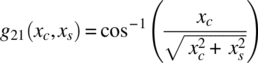
and

Upon evaluating the partial derivatives in (1.211), the Jacobian is found to be15

and, using (1.208), the functions h1(r,θ) and h2(r,θ) are expressed as
and
Substituting (1.216), (1.217), and (1.218) into (1.212) and applying the independence of xc, xs, and φ, as in (1.206), the pdf of the transformed variables r and θ is expressed as

where r ≥ 0, otherwise the pfd is zero, and θ and φ are uniformly distributed over the range 0 ≤ θ, φ ≤ 2π. The pdf for the magnitude r is determined by computing the marginal distribution MR(r) by integrating over the ranges of θ and φ. Defining ψ = θ − φ, the marginal is evaluated as

Davenport and Root [42] point out that the integrand of the bracketed integral is periodic in the uniformly distributed phase ψ and can be integrated over the interval 0 to 2π. With this integration range, the bracketed integral is identified as the zero‐order modified Bessel function expressed as [43]

Therefore, upon using (1.221) and performing the integration over φ, the marginal distribution function MR(r) simplifies, at least in notation, to

Equation (1.222) is the Rice distribution or, as referred to throughout this book, the Ricean distribution that, as developed in the forgoing analysis, characterizes the baseband magnitude distribution of a CW signal with narrowband additive white Gaussian noise. The Ricean distribution also characterizes the magnitude distribution of a received signal from a channel with multipath interference; this channel is referred to as a Ricean fading channel. The Ricean distribution becomes the Rayleigh distribution as A → 0 and the Gaussian distribution as A → ∞; the proof of these two limits is the subject of Problems 19 and 20. The Rayleigh distribution characterizes the amplitude distribution of narrowband noise or, in the case of multipath interference, the composite signal magnitude of many random scatter returns without a dominant specular return or signal component. The multipath interference is the subject of Chapter 18. Defining the signal‐to‐noise ratio as γ = A2/(2σ2), (1.222) is expressed as

The pdf of the phase function is evaluated by computing the marginal distribution MΘΦ(θ,φ) by integrating over the range of the magnitude r. By forming or completing the square of the exponent in the last equality in (1.219) the integration is performed as
Davenport and Root [44] provide an approximate solution to (1.224), under the condition Acos(θ – φ) >> σ. The approximation is expressed as

where γ is the signal‐to‐noise ratio defined earlier. An alternate solution, without the earlier restriction, is expressed by Hancock [45], with ψ = θ − φ, as

where P(z) is the probability integral defined in Section 3.5. Hancock’s phase function is used in Section 4.2.1 to characterize the performance of phase‐modulated waveforms.
As γ → 0 in (1.226) the function fΨ(ψ) → 1/2π resulting in the uniform phase pdf. However, for γ greater than about 3, the probability integral is approximated as [26]

Using (1.227), the phase pdf is approximated as

With |ψ| ≅ 0 such that sin2(ψ) ≅ ψ2 and defining ![]() (1.228) is approximated as
(1.228) is approximated as

Equation (1.229) describes a zero‐mean Gaussian phase pdf with the phase variance ![]() . Hancock’s phase function, expressed in (1.226), is plotted in Figure 4.3 for various signal‐to‐noise ratios.
. Hancock’s phase function, expressed in (1.226), is plotted in Figure 4.3 for various signal‐to‐noise ratios.
1.5.5.2 Distribution of the Product of Two Independent Gaussian Random Variables
In this section the pdf of the product z = xy of two zero‐mean equal‐variance iid Gaussian random variables X and Y is determined. The solution involves defining an auxiliary random variable w = h(x) = x with z = g(x,y) = xy and evaluating fZ,W(w,z) characterized as

where JX,Y(x,y) is the Jacobian of the transformation evaluated as

Using (1.231) and the joint Gaussian pfd of X and Y, expressed by (1.230), with x = w and y = z/w, the marginal pdf of z is evaluated as
However, since X and Y are independent

and, upon substituting x = w and y = z/w into (1.233), (1.232) is expressed as

where the second equality recognizes that the first equality is symmetrical in w. Letting λ = w2/2σ2 (1.234) is expressed as

The solution to the integral in (1.235) appears in the table of integrals by Gradshteyn and Ryzhik (Reference 46, p. 340, pair No. 12) as

where Kv(u) is the modified Bessel function of the second kind of order v. With v = 0 and u = z/σ2, (1.235) is evaluated as

The magnitude of z in (1.237) is used because of the even symmetry of fZ(z) with respect to z. The symmetry of fZ(z) results in a zero‐mean value so the variance is evaluated as

The solution to the integral in (1.238) is found in Gradshteyn and Ryzhik (Reference 46, p. 684, Integral No. 16) and the variance fZ(z) is evaluated as

where the second equality in (1.239) results from the value of the Gamma function ![]() . In Example 4 of Section 1.5.6.1, the pdf of the summation of N iid random variables with pdfs expressed by (1.237) is examined.
. In Example 4 of Section 1.5.6.1, the pdf of the summation of N iid random variables with pdfs expressed by (1.237) is examined.
1.5.6 The Characteristic Function
The characteristic function of the random variable X is defined as the average value of ejvx and is expressed as
With v = −ω and x = t (1.240) is similar to the Fourier transform of a time‐domain function. The characteristic function is also referred to as the moment‐generating function, in that, the nth moment of the random variable X, defined as the expected value E[xn], is evaluated (see Problem 26) as

The Fourier transform relationship between time domain convolution and frequency domain multiplication also applies to the convolution of random variables and the multiplication of the corresponding characteristic functions. Therefore, based on the discussion in Section 1.5.6.1, the summation of N identically distributed (id) random variables corresponds to the product of their individual characteristic functions, that is,

This is a very useful result, in that, the distribution of the summation of N independent random variables is obtained as the inverse transform [47] of (1.242) expressed as
Campbell and Foster [47] provide an extensive listing of Fourier transform pairs defined as
and, by defining v = −2πf, the Fourier transform pairs apply to the transform pairs between fX(x) and CX(v) as expressed in (1.240).
1.5.6.1 Summation of Independently Distributed Random Variables
If two random variables X and Y are independent then the probability density fZ(z) of their sum Z = X + Y is determined from the convolution of fX(x) with fY(y) so that16
For multiple summations of a random variable, the convolution is repeated for each random variable in the summation.
Example 1
Consider the summation of N zero‐mean uniformly distributed random variables Xi expressed as

with
For N = 2 the convolution involves two ranges of the variable z as shown in Figure 1.21 and the integrations are evaluated as
and


FIGURE 1.21 Convolution of two zero‐mean uniform distributions.
Upon evaluation of (1.248) and (1.249) and recognizing the symmetry about z the density function is expressed as

Repeating the application of the convolution for N = 3 and 4 (see Problem 24) results in the probability density functions shown in Figure 1.22 with the corresponding cdf results shown in Figure 1.23. As ![]() the probability density and characteristic functions will approach those of the Gaussian distributed random variable (see Problem 23).
the probability density and characteristic functions will approach those of the Gaussian distributed random variable (see Problem 23).

FIGURE 1.22 pdf for sum of N = 2, 3 and 4 independent zero‐mean uniform distributions (a = 1).

FIGURE 1.23 cdf for sum of N = 2, 3 and 4 independent zero‐mean uniform distributions (a = 1).
The moments of the random variable X are evaluated using the characteristic function
In regions where the characteristic function converges, the moments E[xn] completely define the characteristic function and the pdf of the random variable X, so, upon expanding (1.251) as the power series
the moments are easily evaluated using (1.241). The moments for the random variable Z, formed as in (1.246), are determined using (1.242) and, with Xi : i = 1, …, N iid random variables, the characteristic function for Z is approximated as
The first and second moments for N = 1, …, 4 are listed in Table 1.6. These results are also obtained by evaluating fZ(z) using (1.250) and then evaluating the moments (see Problem 25) as

TABLE 1.6 Moments of fZ(zN) for ![]() , Xi iid Zero‐Mean Uniform Distributions
, Xi iid Zero‐Mean Uniform Distributions
| N | E[z] | E[z2] |
| 1 | 0 | a2/3 |
| 2 | 0 | 2a2/3 |
| 3 | 0 | a2 |
| 4 | 0 | 4a2/3 |
However, it is much easier to use the characteristic function.
Example 2
As another example, consider the summation of N random variables Xi characterized as the sinusoidal function
with constant amplitudes Ai and zero‐mean uniformly distributed phase, expressed as
The resulting pdf of the random variable Xi for ϕ = π, is evaluated in (1.193) as

and is plotted in Figure 1.24.

FIGURE 1.24 pdf of x = Asin(φ) with zero‐mean uniformly distributed phase, A = 1 and ϕ = π.
The pdf of the random variable Z, expressed as in (1.246),17 is evaluated by successive convolutions as in (1.245) and the results for N = 2, 3, and 4 are plotted in Figure 1.25 with the corresponding cdf functions shown in Figure 1.26. The results in Figures 1.25 and 1.26 for N > 1 are obtained by numerical evaluations of the convolutions using incremental values of Δz = 2.5 × 10⁻⁵; this is a reasonable compromise between simulation time and fidelity in dealing with the infinite value at |x| = 1.0.

FIGURE 1.25 pdf of N = 2, 3, and 4 successive convolutions of fX(x).

FIGURE 1.26 cdf of N = 2, 3, and 4 successive convolutions of fX(x).
In this case, the mean and variance of the random variable X are evaluated using the characteristic function of (1.257) found in (Reference 47, p. 123, Transform Pair 914.5); the result is
where Io(−) is the modified Bessel function of order zero. Expanding (1.258) for Av < 1 as a power series, (Reference 46, p. 375, Ascending Series 9.6.10), results in18

and the moments are easily evaluated using (1.241). The first and second moments are listed as the theoretical values in Table 1.7. The moments for the random variable Z, formed as in (1.246) with Xi iid random variables for all i as expressed by the pdf in (1.255), are determined using the characteristic function expressed as

TABLE 1.7 Moments of fZ(zN) for ![]() , Xi iid Random Variables Expressed by (1.255)
, Xi iid Random Variables Expressed by (1.255)
| N | Theoretical | Numericala (A = 1) | ||
| E[z] | E[z2] | E[z] | E[z2] | |
| 1 | 0 | A2/2 | 0 | 0.4999 |
| 2 | 0 | A2 | 0 | 1.0044 |
| 3 | 0 | 3A2/2 | 0 | 1.5055 |
| 4 | 0 | 2A2 | 0 | 2.0146 |
aNumerical values are sampled with Δz = 2.5 × 10⁻⁵.
The corresponding first two moments of the random variable Z for N = 2, 3, and 4 are also listed in Table 1.7. The numerical results listed in Table 1.7 are based on computer evaluations of the various convolutions resulting in the pdfs shown in Figures 1.24 and 1.25.
A major observation in these two examples is that the probability distribution of the random variable Z approaches a Gaussian distribution as N increases (see Problem 27). This is evidence of the central limit theorem which states that (see Davenport and Root, Reference 6, p. 81) the sample mean of the sum of N arbitrarily distributed statistically independent samples becomes normally distributed as N increases. This is referred to the equal‐components case of the central limit theorem. However, as pointed out by Papoulis (Reference 8, p. 266), a consequence of the central limit theorem is that the distribution fZ(z) of the sum of N statistically independent distributions having arbitrary pdf’s tends to a normal distribution as N increases. This is a stronger statement and suggests that the probability P(z) = fZ(Z < z) can be considered a Gaussian distribution for all z as is frequency assumed to be the case in practice. Davenport and Root also point out that, even though N is seemingly large, the tails of the resulting distribution may result in a poor approximation to the Gaussian distribution.
Upon computing the mean and variance using the power series expansion of CZ(v) expressed by (1.252) with av << 1, the approximate expression for the corresponding Gaussian distribution is easily obtained. After summing N uniformly distributed amplitudes the expression for the pdf is

Similarly, for the summation of N sinusoids with Av << 1, the pdf in Example 2 is expressed as

It is interesting to note that the second moments are Nλ2 for all values of N including those for which the pdf does not have the slightest resemblance to the Gaussian pdf. In these cases, the important difference is that the corresponding probabilities P(x) = FX(X < x) are entirely different from those of the Gaussian distribution with the possible exception of the median value. Finally, it is noted that the limiting behavior for λv << 1 and N → ∞ applies to the summation of independently distributed distributions that may, or may not, be identically distributed distributions.
Example 3
This example involves the summation of random chips {±1} in a direct‐sequence spread‐spectrum (DSSS) waveform. In this case, the chips occur with equal probabilities according to the pdf expressed as
Using (1.240), the characteristic function is evaluated as

The DSSS waveform uses N chips per bit and the demodulator correlation sums the N chips to form the correlation output ![]() with the corresponding characteristic function given by
with the corresponding characteristic function given by

To evaluate the first and second moments of y only the first two terms in the expansion of cosN(v) are required and, upon using (1.241), these moments are evaluated as

and

The variance of y is defined as the second central moment ![]() and with zero‐mean the variance is
and with zero‐mean the variance is ![]() .
.
Example 4
The pdf fZ(z) of the product of two, zero‐mean, equal‐variance, iid Gaussian random variables, z = xy, is expressed in (1.237) as a function of the zero‐order modified Bessel function Ko(|z|/σ2) where the magnitude of z provides for the range: −∞ ≤ z ≤ ∞. In this example, the pdf ![]() is evaluated where
is evaluated where ![]() : i = 1, …, N. The evaluation is based on the N‐th power of the characteristic function CZ(v) and, from the work of Campbell and Foster (Reference 47, p. 60, pair No. 558), the characteristic function is evaluated as19
: i = 1, …, N. The evaluation is based on the N‐th power of the characteristic function CZ(v) and, from the work of Campbell and Foster (Reference 47, p. 60, pair No. 558), the characteristic function is evaluated as19

The characteristic function of ![]() is the N‐th power of (1.268) expressed as
is the N‐th power of (1.268) expressed as

and, using the transform pair of Campbell and Foster (Reference 47, p. 61, pair No. 569.0), the pdf of ![]() is evaluated as
is evaluated as

As in the case for fZ(z), the pdf ![]() applies for −∞ ≤
applies for −∞ ≤ ![]() ≤ ∞ and is symmetrical with respect to
≤ ∞ and is symmetrical with respect to ![]() resulting in a zero‐mean value with the variance expressed as
resulting in a zero‐mean value with the variance expressed as

The solution to the integral in (1.271) is found in Gradshteyn and Ryzhik (Reference 46, p. 684, Integral No. 16) and the variance fZ(z) is evaluated using

Substituting the solution to the integral in (1.272) into (1.271), with u = (N + 3)/2, v = (N − 1)/2, and a = 1/σ2, the solution to variance simplifies to
In the earlier evaluation, the integer argument Gamma function is related to the factorial as ![]() ! and
! and ![]() . This result could also be evaluated using the movement generating function of (1.241), however, using the integral solution as in (1.272) it is sometimes easier to evaluate the moments. With a sufficiently large value of N the pdf
. This result could also be evaluated using the movement generating function of (1.241), however, using the integral solution as in (1.272) it is sometimes easier to evaluate the moments. With a sufficiently large value of N the pdf ![]() is approximated as the Gaussian pfd expressed as
is approximated as the Gaussian pfd expressed as
The probability density functions discussed earlier and others encountered in the following chapters are summarized in Table 1.8 with the corresponding mean values, variances, and characteristic functions.
TABLE 1.8 Probability Distributions and Characteristic Functions
| Name | fX(x) | E[x] | Var[x] | CX(v) | Conditions |
| Uniform |  |
||||
| Bernoulli |  |
p | p(1 − p) | (1 − p) + pv | Discrete binary variable x = ki : i = 1, 2 |
| Binomial |  |
np | np(1 – p) | Discrete variable |
|
| Poisson | α | α | Discrete variable |
||
| Exponential | 1/α | 1/α2 | |||
| Gaussian (normal) |  |
m | σ2 | ||
| Chi‐square (N = 2) Exponential (α = 1/2) |
2 | 4 | x ≥ 0 | ||
| Chi‐squared (N‐degrees) |  |
N | 2N | N‐degrees of freedom x ≥ 0 | |
| Rayleigh | x > 0 | ||||
| Ricean |  |
a | a | a | x > 0 |
| Gamma |  |
α/β | α/β2 |  |
x > 0 β > 0; λ > 0 |
| Lognormal |  |
 |
b | y is lognormal y = ex ≥ 0 x = N(m,σ) |
|
| Nakagami‐m |  |
c | c | c | x ≥ 0 |
Notes: γ = A2/(2σ2) is the signal‐to‐noise ratio. γ→0 fX(x) = Rayleigh with E[x] = ![]() , Var[x] =
, Var[x] = ![]() .
.
aγ→∞ fX(x) = Gaussian with E[x] = A, Var[x] = σ2.
bApproximated using a series expansion of ejvy.
cRefer to special cases in Section 1.5.7.2.
1.5.7 Relationships between Distributions
In the following two subsections, the relationship between various probability density functions is examined by straightforward parameter transformations, allowing parameters to approach limits, or simply altering various parameter values. The most notable relationship is based on the central limit theorem in which a distribution approaches the Gaussian distribution by increasingly summing the operative random variable.
1.5.7.1 Relationship between Chi‐Square, Gaussian, Rayleigh, and Ricean Distributions
A random variable has a chi‐square (χ2) distribution with N degrees of freedom if it has the same distribution as the sum of the squares of N‐independent, normally distributed random variables, each with zero‐mean and unit variance.20
Consider the zero‐mean Gaussian or normal distributed random variable x with variance ![]() and pdf expressed as
and pdf expressed as
The pdf of a new random variable y = x2, obtained by simply squaring x, is determined by considering the positive and negative regions of ![]() as shown in Figure 1.27.
as shown in Figure 1.27.

FIGURE 1.27 Transformation of the random x to y = x2.
The pdf of y is determined using the incremental intervals dy = 2xdx at ![]() such
such

The characteristic function of (1.276) is evaluated as

Consider now the random variable z resulting from the summation of N independent random variables yi such that

The characteristic function of z is simply the N‐th power of CY(v) so that

Equation (1.279) transforms to the pdf of z, resulting in

In conforming to the earlier definition, the chi‐square distribution is expressed by letting ![]() in (1.280) or, more formally, using the transformation
in (1.280) or, more formally, using the transformation ![]() ; therefore, the pdf of the chi‐square random variable χ with N degrees of freedom is
; therefore, the pdf of the chi‐square random variable χ with N degrees of freedom is

and the corresponding characteristic, or moment generating, function is

Equation (1.281) is occasionally referred to as the central χ2 distribution because it is based on noise only, that is, the underlying zero‐mean Gaussian random variables xi with distribution given by (1.275) do not contain a signal component.21
Special Case for N = 2
Under this special case ![]() (1.280) reduces to the exponential distribution
(1.280) reduces to the exponential distribution

So the resulting chi‐square χ2 distribution is obtained from (1.281) with N = 2. This is an important case because x1 and x2 can be thought of as orthogonal components in the complex description of a baseband data sample. Urkowitz [48] shows that the energy of a wide‐sense stationary narrowband white noise Gaussian random process with bandwidth –W to W Hz and measured over a finite interval of T seconds is approximated by N = 2WT terms or degrees of freedom. The frequency W is the noise bandwidth of the narrowband baseband filter and the approximation error in the energy measurement decreases with increasing 2WT. The factor of two can be thought of as the computation of complex orthogonal baseband functions ![]() so N = 2 degrees of freedom correspond to WT = 1. For example, the rect(t/T) function observed over the interval T seconds has a noise bandwidth of W = 1/T Hz corresponding to WT = 1 resulting in 2 degrees of freedom.
so N = 2 degrees of freedom correspond to WT = 1. For example, the rect(t/T) function observed over the interval T seconds has a noise bandwidth of W = 1/T Hz corresponding to WT = 1 resulting in 2 degrees of freedom.
Upon letting ![]() , the random variable w is described in terms of the Rayleigh distribution
, the random variable w is described in terms of the Rayleigh distribution
So the Rayleigh distribution is derived from the magnitude of the quadrature zero‐mean Gaussian distributed random variables, x = N(0,σ).22
1.5.7.2 Relationship between Nakagami‐m, Gaussian, Rayleigh, and Ricean Distributions
The Nakagami‐m distribution [49] was initially derived from experimental data to characterize HF fading; however, subsequent experimental observations demonstrate its application to rapid fading at carrier frequencies from 200 MHz to 4 GHz. It is considered to be a generalized distribution from which other distributions can be derived, for example, m = 1 results in the Rayleigh power distribution, m = ½ results in the one‐sided zero‐mean Gaussian distribution, and as ![]() the m‐distribution approaches the Gaussian distribution with a unit mean value. In the region 1 ≤ m ≤ ∞, the Nakagami‐m distribution behaves much like the Ricean distribution; however, the normalized distributions are subtly different when plotted for various signal‐to‐noise ratios less than about 10 dB. The Ricean distribution, referred to as the n‐distribution by Nakagami, is derived from concepts involving narrowband filtering of a continuous wave (CW) signal with additive Gaussian noise, whereas the Nakagami‐m distribution is derived from experimental data involving multipath communication links.
the m‐distribution approaches the Gaussian distribution with a unit mean value. In the region 1 ≤ m ≤ ∞, the Nakagami‐m distribution behaves much like the Ricean distribution; however, the normalized distributions are subtly different when plotted for various signal‐to‐noise ratios less than about 10 dB. The Ricean distribution, referred to as the n‐distribution by Nakagami, is derived from concepts involving narrowband filtering of a continuous wave (CW) signal with additive Gaussian noise, whereas the Nakagami‐m distribution is derived from experimental data involving multipath communication links.
1.5.8 Order Statistics
Communication systems analysis and performance evaluations often involve a large number of random samples taken from an underlying continuous or discrete probability distribution function. The various parameters, used to characterize the system performance, result in limiting distributions with associated means, variances, and confidence levels as dictated, for example, by an underlying distribution. Order statistics [31, 50, 51], on the other hand, involves a distribution‐free or nonparametric analysis that requires only that the probability distribution functions be continuous and not necessary related to the underlying distribution from which the samples are taken. However, the randomly drawn samples are considered to be statistically independent.
Consider that the n random samples {X1, X2, …, Xn} are taken from the continuous pdf fX(x) over the range ![]() . Now consider reordering the random variables Xi : i = 1, …, n to form the random variables {Y1, Y2, …, Y n} arranged in ascending order of magnitude, such that,
. Now consider reordering the random variables Xi : i = 1, …, n to form the random variables {Y1, Y2, …, Y n} arranged in ascending order of magnitude, such that, ![]() where
where ![]() is uniformly distributed over the interval b − a. The joint pdf of the ordered samples [52] is expressed as
is uniformly distributed over the interval b − a. The joint pdf of the ordered samples [52] is expressed as

for ![]() and n! is the number of mutually disjoint sets of x1, x2, …, xn. For example, for n = 4 the set x1, x2, x3, x4 results in n! = 24 mutually disjoint sets determined as shown in Table 1.9. The first six mutually disjoint sets are determined by cyclically left shifting the indicated subsets of original set x1, x2, x3, x4; a cyclic left shift of a subset is obtained by shifting each element of the subset to the left and replacing the leftmost element in the former position of the rightmost element. Following the first six sets shown in the figure, the original set is cyclically shifted three more times each leading to six mutually disjoint sets by shifting subsets resulting in a total of 24 mutually disjoint sets.
and n! is the number of mutually disjoint sets of x1, x2, …, xn. For example, for n = 4 the set x1, x2, x3, x4 results in n! = 24 mutually disjoint sets determined as shown in Table 1.9. The first six mutually disjoint sets are determined by cyclically left shifting the indicated subsets of original set x1, x2, x3, x4; a cyclic left shift of a subset is obtained by shifting each element of the subset to the left and replacing the leftmost element in the former position of the rightmost element. Following the first six sets shown in the figure, the original set is cyclically shifted three more times each leading to six mutually disjoint sets by shifting subsets resulting in a total of 24 mutually disjoint sets.
TABLE 1.9 Example of Mutually Disjoint Sets (n = 4, 24 Mutually Disjoint Sets)
| No. | Mutually Disjoint Sets | Shiftinga |
| 1 | x1, x2, x3, x4 | Original set |
| 2 | x1, x2, x4, x3 | Shift subset x3, x4 |
| 3 | x1, x3, x4, x2 | Shift subset x2, x3, x4 |
| 4 | x1, x3, x2, x4 | Shift subset x4, x2 |
| 5 | x1, x4, x2, x3 | Shift subset x3, x4, x2 |
| 6 | x1, x4, x3, x2 | Shift subset x2, x3 |
| 7 | x2, x3, x4, x1 | Shift original set |
| 8 | x2, x3, x1, x4 | Shift subset x4, x1 |
| 9 | x2, x4, x1, x3 | Shift subset x3, x4, x1 |
| ⋯ | ⋯ | ⋯ |
aShift denotes a cyclic left shift of a previous set or subset.
The ordered sample Yi is referred to as the i‐th order statistic of the sample set. The marginal pfd of the n‐th order statistic Yn, that is, the maximum of {X1, X2, …, Xn}, is evaluated using (1.285) by performing the integrations in the ascending order i = 1, 2, …, n − 1 as follows23:

The solution (see Problem 15) to (1.286) is
where Fn−1(yn) is the cdf evaluated as
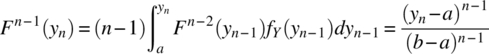
Using the marginal pdf of Yn given by (1.287), the probability of selecting the maximum of value Yn is determined as

These results are distribution free, in that, the pdf has not been defined; however, from a practical point of view (1.289) can be evaluated for any continuous pdf.
The distributions from which the xi are taken need not be identical24; for example, the samples x1 through xj can be taken from a distribution involving signal plus noise (or clutter) and those from xj+1 through xn corresponding to noise (or clutter) only. Using this example the distribution in (1.287) is expressed as
where Fsn(y) is the distribution corresponding to signal plus noise and Fn(y) is the noise‐only distribution.
Example distributions used to evaluate the performance of communication and radar systems are Gaussian, Ricean, lognormal, and Weibull distributions. Table 1.10 lists the false‐detection probabilities, for the indicated signal‐to‐noise ratios γdB, associated with the detection of j = 1 signal‐plus‐noise event and k = n − j = (1,2,4, and 8) noise‐only events.
TABLE 1.10 Order Statistics False‐Detection Probability for Gaussian Distributed Random Variables
| Ordered S + N and N Statistics (j,k) | False‐Detection Probability (Pfd) | ||
| γdB = 10 | γdB = 15 | γdB = 20 | |
| 1,1 | 2.440e−2 | 6.645e−5 | 1.408e−12 |
| 1,2 | 4.226e−2 | 1.308e−4 | 2.815e−12 |
| 1,4 | 6.980e−2 | 2.547e−4 | 5.629e−12 |
| 1,8 | 1.089e−1 | 4.874e−4 | 1.126e−11 |
1.5.9 Properties of Correlation Functions
Correlation processing is used in nearly every aspect of demodulator signal detection from energy detection, waveform acquisition, waveform tracking, parameter estimation, and information recovery processing. With this wide range of applications, the theoretical analyst, algorithm developer, software coder, and hardware developer must be thoroughly familiar with the properties and implementation of waveform correlators. An equally important processing function is that of convolution or linear filtering. The equivalence between matched filtering and correlation is established in Section 1.7.2 and involves a time delay in the correlation response; with this understanding, the properties of correlation can be applied to convolution or filtering. The correlation response can be exploited to determine the signal signature regarding the location of a signal in time and frequency, the duration and bandwidth of the signal, the shape of the modulated signal waveform, and the estimate of the information contained in the modulated waveform.
The correlation function25 is evaluated for the complex functions ![]() as the integral
as the integral
and
where the asterisk denotes complex conjugation.
Autocorrelation processing examines the correlation characteristics of a single random process with the maximum magnitude corresponding to the zero‐lag condition ![]() that is equal to the maximum energy over the correlation interval. The correlation response
that is equal to the maximum energy over the correlation interval. The correlation response ![]() is indicative of the shape of
is indicative of the shape of ![]() and the duration, τd, of the principal correlation response is indicative of the correlation time. For deterministic signals, the correlation time (τo) is usually characterized in terms of the one‐sided width of the principal correlation lobe; however, for stochastic processes the correlation interval is defined when |
and the duration, τd, of the principal correlation response is indicative of the correlation time. For deterministic signals, the correlation time (τo) is usually characterized in terms of the one‐sided width of the principal correlation lobe; however, for stochastic processes the correlation interval is defined when |![]() | decreases monotonically from
| decreases monotonically from ![]() to a defined level; for example, when the normalized correlation response first reaches the level
to a defined level; for example, when the normalized correlation response first reaches the level ![]() . The normalized correlation response is referred to as the correlation coefficient as defined in (1.295) or (1.296). The parameters related to the correlation of the function
. The normalized correlation response is referred to as the correlation coefficient as defined in (1.295) or (1.296). The parameters related to the correlation of the function ![]() have equivalent Fourier transform frequency‐domain definitions. In the case of stochastic processes, the Fourier transform of
have equivalent Fourier transform frequency‐domain definitions. In the case of stochastic processes, the Fourier transform of ![]() is defined as the PSD of the process.
is defined as the PSD of the process.
Expanding (1.292) in terms of the real and imaginary with ![]() and
and ![]() results in
results in

This evaluation requires four real multiplies and integrations for each lag, whereas, if ![]() and ỹ(t) were real functions only one multiplication and integration is required for each lag. With discrete‐time sampling, the integrations are replaced by summations over the finite sample values
and ỹ(t) were real functions only one multiplication and integration is required for each lag. With discrete‐time sampling, the integrations are replaced by summations over the finite sample values ![]() and ỹn where t = nTs: n = 0, …, N − 1 and Ts is the sampling interval; in this case, the computational complexity is proportional to N2. The computation complexity can be significantly reduced by performing the correlation in the frequency domain using FFT [53], in which case, for a radix‐2 FFT with N = 2k, the computation complexity is proportional to Nlog2(N). Brigham [54] provides detailed descriptions of the implementation and advantages of FFT correlation and convolution processing. The correlation results throughout the following chapters use the direct and FFT approaches without distinction.
and ỹn where t = nTs: n = 0, …, N − 1 and Ts is the sampling interval; in this case, the computational complexity is proportional to N2. The computation complexity can be significantly reduced by performing the correlation in the frequency domain using FFT [53], in which case, for a radix‐2 FFT with N = 2k, the computation complexity is proportional to Nlog2(N). Brigham [54] provides detailed descriptions of the implementation and advantages of FFT correlation and convolution processing. The correlation results throughout the following chapters use the direct and FFT approaches without distinction.
Referring to (1.291) the zero‐lag correlation is expressed as

where Ex is the total energy in the received signal. Using (1.294), the normalized correlation is defined in terms of the normalized autocorrelation coefficient as
with |ρx(τ)| ≤ 1. From (1.292), the normalized cross‐correlation coefficient is defined as

with |ρxy(τ)| ≤ 1.
The correlation may also be defined in terms of the long‐term average over the interval T as

However, most practical waveforms are limited to a finite duration Tc = NTs and, in these cases, ![]() is zero outside of the range Tc. Therefore, dividing the zero‐lag correlation by Tc results in the second‐order moment
is zero outside of the range Tc. Therefore, dividing the zero‐lag correlation by Tc results in the second‐order moment ![]() where
where ![]() is the DC or mean signal power. Removing the mean signal level prior to performing the correlation results in the autocovariance with
is the DC or mean signal power. Removing the mean signal level prior to performing the correlation results in the autocovariance with ![]() . Table 1.11 summarized several properties of correlation functions.
. Table 1.11 summarized several properties of correlation functions.
TABLE 1.11 Correlation Function Properties of Deterministic and Stochastic Processes
| Property | Comments |
| Autocorrelation | |
| x(t) is real | |
| Autocovariance | |
| Cross‐covariance | |
Consider, for example, that ![]() is a received signal plus AWGN, the correlation
is a received signal plus AWGN, the correlation ![]() is performed in the demodulator using the known reference signal
is performed in the demodulator using the known reference signal ![]() . The dynamic range of the demodulator detection processing is minimized by the normalization in (1.296) and the optimum signal detection corresponds to ρxy(0). On the other hand, if the optimum timing is not known, near optimum detection can be achieved by choosing the maximum correlation output over the uncertainty range of the correlation lag about τ = 0. During initial signal acquisition, the constant false‐alarm rate (CFAR) threshold, described in Section 11.2.2.1, is an effective algorithm for signal presence detection and coarse synchronization.
. The dynamic range of the demodulator detection processing is minimized by the normalization in (1.296) and the optimum signal detection corresponds to ρxy(0). On the other hand, if the optimum timing is not known, near optimum detection can be achieved by choosing the maximum correlation output over the uncertainty range of the correlation lag about τ = 0. During initial signal acquisition, the constant false‐alarm rate (CFAR) threshold, described in Section 11.2.2.1, is an effective algorithm for signal presence detection and coarse synchronization.
1.6 RANDOM PROCESSES
Many of the signal descriptions and processing algorithms in the following chapters deal exclusively with the signal and neglect the additive noise under the reasoning that the noise detracts from the fundamental signal processing requirements and complicates the notation which has the same effect. On the other hand, understanding the impact of the noise on the system performance is paramount to the waveform selection and adherence to the system performance specifications. To this end, the performance evaluation is characterized by detailed analysis of the signal‐plus‐noise conditions and confirmed by computer simulations.
The following descriptions of noise and signal plus noise are provided to illustrate the assumptions and analysis associated with the inclusion of the most basic noise source—AWGN. The reference to narrowband Gaussian noise simply means that the carrier frequency fc is much greater than the signal modulation Nyquist bandwidth BN so that the 2fc heterodyning or homodyne mixing terms are completely eliminated through filtering. In such cases, the white noise in the baseband demodulator bandwidth is denoted by the single‐sided noise density No watts/Hz, where single‐sided refers to positive frequencies.
1.6.1 Stochastic Processes
The subject of stochastic processes is discussed in considerable detail by Papoulis [55] and Davenport and Root [56] and the following definitions are often stated or implied in the applications discussed in throughout the following chapters. A stochastic process is defined as a random variable that is a function of time and the random events χ in S as depicted in Figure 1.14. In this context the random variable is characterized as x(t,χ). For a fixed value of t = ti, x(ti,χ) is a random variable and χ = χi, x(t,χi) denotes as the real random process x(t) such that x(ti) is a random variable with pdf fX(x:ti); in general, the pdf of x(t) is defined as fX(x:t).
1.6.1.1 Stationarity
There are several ways to define the stationarity of a stochastic process, for example, stationarity of finite order, asymptotic stationary, and periodic stationarity; however, the following two are the most frequently encountered.
Strict‐Sense Stationary Process
The stochastic process x(t) is strict‐sense stationary, or simply stationary, if the statistics are unaltered by a shift in the time axis. Furthermore, two random variables are jointly stationary if the joint statistics are unaltered by an equal time shift of each random variable, that is, the probability density function f(x ; t) is the same for all time shifts τ. This is characterized as
Wide‐Sense Stationary Process
The stochastic process x(t) is wide‐sense stationary (WSS) if its expected value is constant and autocorrelation function is a function of the time shift τ = t2 − t1 ∀ t1 and t2. WSS stationarity is characterized as
and
Because wide‐sense stationarity depends on only the first and second moments it is also referred to as weak stationarity. A function of two random processes is wide‐sense stationary if each process is wide‐sense stationary and their cross‐correlation function is dependent only the time shift, that is,
1.6.1.2 Ergodic Random Process
The random process x(t), defined earlier, is an ergodic random process if the statistics of x(t) are completely defined by the statistics of x(t,χ). Denoting the random process x(ti,χ) as an ensemble of x(t,χ), then ergodicity ensures that the statistics x(ti) are identical to those of the ensemble; in short, the time statistics are identical to the ensemble statistics.26 Ergodicity of the mean, of the stochastic process x(t,χ), exists under the condition
where the time average is defined as

and the ensemble average is defined as
Since the mean value of a random process must be a constant, the ergodic of the mean theorem states that the equality condition in (1.302) is satisfied when ![]() where η is a constant. This is a nontrivial task to prove, however, following the discussion by Papoulis [57], the ergodic of the mean theorem states that
where η is a constant. This is a nontrivial task to prove, however, following the discussion by Papoulis [57], the ergodic of the mean theorem states that

The iff condition in (1.305) is formally expressed in terms of the autocovariance function for which the limit T → ∞ is expressed as the variance ![]() . However, from (1.305), the expectation E[x(t)] = η resulting in
. However, from (1.305), the expectation E[x(t)] = η resulting in ![]() . Therefore, the limit T → ∞ of the autocovariance function converges in probability with the conclusion that
. Therefore, the limit T → ∞ of the autocovariance function converges in probability with the conclusion that ![]() proving ergodicity of the mean.27 Demonstration of ergodicity of the autocorrelation function is considerably more involved, requiring the fourth‐order moments.
proving ergodicity of the mean.27 Demonstration of ergodicity of the autocorrelation function is considerably more involved, requiring the fourth‐order moments.
1.6.2 Narrowband Gaussian Noise
Consider the noise described by the narrowband process [58] with bandwidth B << fc expressed as
where N(t) and θ(t) represent, respectively, the envelop and phase of the noise and ωc = 2πfc is the angular carrier frequency. Upon expanding the trigonometric functions, (1.306) can also be expressed as
where
and
The noise terms nc(t) and ns(t) are uncorrelated with spectrum S(f) and bandwidth B, such that S(f) = 0 for |f − fc| > B/2. This is the general characterization of a narrowband noise process; however, in the following analysis, nc(t) and ns(t) are also considered to be statistically independent, stationary zero‐mean white noise Gaussian processes with one‐sided spectral density No watts/Hz.
Because of the stationarity, the noise autocorrelation is dependent only on the correlation lag τ and is evaluated as

Upon evaluating the product in (1.310) and distributing the expectation, it is found that the conditions for stationarity require28 Rss(τ) = Rcc(τ) and Rcs(τ) = −Rsc(τ) so that (1.310) reduces to
The noise power is evaluated using (1.311) with τ = 0 with the result Rnn(0) = Rcc(0) = ![]() . This evaluation can be carried further using the Wiener–Khinchin theorem29 which states that the power spectral density of a WSS random process is the Fourier transform of the autocorrelation function, that is,
. This evaluation can be carried further using the Wiener–Khinchin theorem29 which states that the power spectral density of a WSS random process is the Fourier transform of the autocorrelation function, that is,
From (1.312) the inverse Fourier transform is
and, substituting the condition that the single‐sided noise spectral density is defined as No watts/Hz, (1.313) becomes
In (1.314) the single‐sided noise density is divided by two because of the two‐sided integration, that is, the integration includes negative frequencies. In this case, the noise power, defined for τ = 0, is infinite, however, when the ideal band‐limited filter, with bandwidth B, is considered the noise power in the filter centered at fc is computed as

In this case the one‐sided noise density No is used instead of No/2 because the one‐sided integration is over positive frequencies.
If a linear filter with impulse response h(t) is used, the frequency response is given by
The corresponding unit gain normalizing factor is |H(0)|. With the stationary noise process n(t) applied to the input of the filter, the output is determined using the convolution integral and the result is as follows:
Using (1.317) it can be shown (see Problem 33) that the normalized spectrum of the output noise is expressed, in terms of the input noise PSD Sn(f), as

where |H(0)| is the normalizing gain of the filter. Using (1.318), with Sn(f) = No/2 corresponding to white noise, the output noise power is evaluated as

where the second integral in (1.319) is recognized as the definition of the noise bandwidth of the bandpass filter with lowpass bandwidth Bn.
1.7 THE MATCHED FILTER
The problem in the detection of weak signals in noise is one of deciding whether the detection filter output is due to the signal and noise or simply noise only. The matched filter [59, 60], provides for the optimum signal detection in AWGN noise based on the maximum instantaneous signal‐to‐noise ratio when sampled at the optimum time.30 The matched filter, for an AWGN channel, is characterized as having an impulse response equal to the delayed time‐reverse replica of the received signal. To maximize the signal detection probability the matched filter output must be sampled at To as defined in the following analysis. The matched filter can be implemented at a convenient receiver IF or in the demodulator using quadrature baseband‐matched filters.
Considering the received signal, sr(t), the matched filter impulse response depicted in Figure 1.28 is expressed as

FIGURE 1.28 Example received signal and corresponding matched filter.
The gain G is selected for convenience; however, it must be a constant value. The delay To is required to result in a causal impulse response, that is, the response of h(t ≤ 0) = 0 for h(t) to be realizable; consequently, sr(t ≥ To) must be zero. Usually the selection of To is not an issue since many symbol modulation functions are time limited or can be truncated without a significant impact on the transmitted signal spectrum; however, the matched filter delay results in a throughput delay. To the extent that the impulse approximates (1.320) a detection loss will be encountered.
The criterion of the matched filter is to provide the maximum signal‐to‐noise ratio in the AWGN channel when sampled at the optimum time To. The following matched filter analysis follows that of Skolnik [61]. The signal‐to‐noise ratio of interest is
where ![]() is evaluated as
is evaluated as

and N is the noise power evaluated as
In these expressions, the filter spectrum H(f) is normalized, such that H(0) = 1, and the last equality in (1.323) results because the channel noise is white with one‐sided constant power density of No watts/Hz. Substituting (1.322) and (1.323) into (1.321) results in the expression for the signal‐to‐noise ratio

The maximum signal‐to‐noise ratio is evaluated by applying Schwarz’s inequality (see Section 1.14.5, Equation 5) to the numerator of (1.324). Upon substituting ![]() and
and ![]() into the Schwarz inequality, (1.324) is expressed as
into the Schwarz inequality, (1.324) is expressed as

The equality condition of the signal‐to‐noise ratio in (1.325) applies when f(f) = cg(f), where c > 0 is a conveniently selected constant resulting in the matched filter frequency response expressed as
where G = 1/c is an arbitrarily selected constant gain greater that zero. Upon applying Parseval’s theorem and recognizing that the numerator of the second equality in (1.325) is the signal energy, E, the optimally sampled matched filter output signal‐to‐noise ratio is simply expressed as
Therefore, for the AWGN channel, the optimally sampled matched filter output results in a signal‐to‐noise ratio that is a function the signal energy and noise density and is independent of the shape of the signal waveform. The factor of two in (1.327) results from the analytic or baseband signal description in the derivation of the matched filter. Typically, the received signal spectrum is modulated onto a carrier frequency with an average power equal to one‐half the peak carrier power. In this case, the signal‐to‐noise ratio at the output of the matched filter is one‐half of that in (1.327) resulting in
Referring to (1.326), the inverse Fourier transform of the complex conjugate of the signal spectrum results in the filter impulse response corresponding to the time reverse of the signal. In addition, the inverse Fourier transform of the exponential function in (1.326) results in a signal time delay of To seconds, so the resulting filter impulse response, h(t), corresponds to the example depicted in Figure 1.28. Consequently, the matched filter impulse response can be expressed in the time domain by (1.320) or in the frequency domain by (1.326).
The detection loss associated with a filter that is not matched to the received signal is evaluated as

where ![]() and
and ![]() are the output signal and mean noise power density at the output of the unmatched filter. Typically the matched filter is based on the transmitted waveform; however, the received signal into the matched filter may be distorted by the channel or receiver filtering31 resulting in a detection loss. The matched filter implementation may also result in design compromises that result in a detection loss.
are the output signal and mean noise power density at the output of the unmatched filter. Typically the matched filter is based on the transmitted waveform; however, the received signal into the matched filter may be distorted by the channel or receiver filtering31 resulting in a detection loss. The matched filter implementation may also result in design compromises that result in a detection loss.
1.7.1 Example Application of Matched Filtering
In this example, a BPSK‐modulated received signal is considered with binary source data bits bi = {0,1} expressed as the unipolar data di = (1 − 2bi) = {1,−1} over the data intervals ![]() of the bit duration T. The received signal plus noise is expressed as
of the bit duration T. The received signal plus noise is expressed as
The signal is described as
The noise is zero‐mean additive white Gaussian noise with one‐sided spectral density No described as
The receiver‐matched filter impulse response and Fourier transform are given by
In (1.333) the signal spectrum defined as S(f) and the squared magnitude of the matched filter output at the optimum sampling point is

where the gain G = |H(0)| is normalized to one resulting in a unit gain‐matched filter response H(f).
Referring to the additive noise described by (1.332) and Section 1.6.2, the noise power at the output of the matched filter is expressed as

where B/2 is the baseband bandwidth of the matched filter.
The received signal, as expressed in (1.330), can be rewritten in terms of the optimally sampled matched filter output as

where ni are iid zero‐mean, unit variance, white Gaussian noise samples. Upon dividing (1.336) by ![]() the sampled matched filter output is expressed as
the sampled matched filter output is expressed as

The sampled values l(r(iTo)) and l′(ri) are referred to as sufficient statistics, in that, they contain all of the information in r(t), expressed in (1.330), to make a maximum‐likelihood estimate ![]() of the source‐bit di. The normalized form in (1.337) is used as the turbo decoder input discussed in Section 8.12. In Section 1.8 the sufficient statistic is seen to be a direct consequence of the log‐likelihood ratio.
of the source‐bit di. The normalized form in (1.337) is used as the turbo decoder input discussed in Section 8.12. In Section 1.8 the sufficient statistic is seen to be a direct consequence of the log‐likelihood ratio.
1.7.2 Equivalence between Matched Filtering and Correlation
Consider the receiver input as the sum of the transmitted signal plus noise expressed as
The cross‐correlation of r(t) with a replica of the received signal is computed as
Defining the matched filter impulse response as h(t), the matched filter output response to the input r(t) is
However, referring to the preceding matched filter discussion, the matched filter response is equal to the delayed image of the signal, such that,
As mentioned previously, the delay To ensures that the filter response is causal and, therefore, realizable. To substitute (1.341) into (1.340) first let ![]() so that
so that ![]() and substitute this result in (1.340) to get
and substitute this result in (1.340) to get

So that the convolution response is equal to the cross‐correlation response delayed by To. If the input noise is zero, so that r(t) = s(t), the same conclusion can be drawn regarding the autocorrelation response.
1.8 THE LIKELIHOOD AND LOG‐LIKELIHOOD RATIOS
Bayes criterion is based on two events, referred to as hypothesis H1 and H0, that are dependent upon a priori probabilities P1 and P0 and the, respective, associated costs (C01,C11) and (C10,C00). Letting m correspond to the decision and n correspond to the hypothesis, the range of the cost is 0 ≤ Cmn ≤ 1 with Cmn + Cnn|m≠n = 1. The cost of a correct decision is Cnn and an incorrect decision is Cmn|m≠n. For communication links the cost of incorrect decision is typically higher than a correct decision so that Cmn|m≠n > Cnn. For example, when Cmn|m≠n = 1 and Cnn = 0 the decision threshold minimizes the probability of error which is the goal of communication demodulators. In summary,

and the a priori probabilities are typically known and equal.
In the following example, the hypotheses correspond to selecting di = {1,−1}, such that, under the two hypotheses

with the observations
corresponding to the optimally sampled outputs of the matched filter. In terms of the a priori, the transition probabilities, and the cost functions, the hypothesis H1: with di = 1 is chosen if the following inequality holds,
otherwise, chose H0 with di = −1. The decisions are made explicit under the following rearrangement of (1.346)

Left and right sides of (1.347) are defined as the likelihood ratio (LR) Λ(r) and decision threshold η or, alternately, as the log‐likelihood ratio (LLR) lnΛ(r) with the threshold lnη, so (1.347) is also expressed as

1.8.1 Example of Likelihood and Log‐Likelihood Ratio Detection
Consider the two hypotheses H1 and H0 mentioned earlier with di = {1,−1} and the observation ri in (1.345) with the additive noise ni characterized as iid zero‐mean white Gaussian noise, denoted as N(0,σn). The transition probabilities are expressed in terms of the Gaussian noise pdf as
Upon forming the likelihood ratio and recognizing that ![]() = ±di, the likelihood ratio decision simplifies to
= ±di, the likelihood ratio decision simplifies to

and the log‐likelihood ratio decision simplifies to

Recognizing that l(ri) is a sufficient statistic, (1.351) is rewritten as

When C10 = C01 = 1, C00 = C11 = 0, and P0 = P1 the LLR simplifies to

Therefore, the data estimate is ![]() when l(ri) > 0, otherwise,
when l(ri) > 0, otherwise, ![]() . Recall that observations ri : t = iTo are made at the output of the matched filter. These concepts involving the LR and LLR surface again in Section 3.2 and the notion of the natural logarithm of the transitions probabilities is discussed in the following section involving parameter estimation.
. Recall that observations ri : t = iTo are made at the output of the matched filter. These concepts involving the LR and LLR surface again in Section 3.2 and the notion of the natural logarithm of the transitions probabilities is discussed in the following section involving parameter estimation.
1.9 PARAMETER ESTIMATION
The subject of optimum signal detection in noise was examined in the preceding section in terms of a pulsed‐modulated carrier and it resurfaces throughout the following chapters in the context of a number of different waveform modulations. However, signal detection is principally based on the signal energy without regard to specific signal parameters, although frequency and range delay must be estimated to some degree to declare signal presence and subsequently detection. Signal detection uses concepts involving direct probabilities, whereas the subject of parameter estimation uses concepts involving inverse probabilities as discussed by Feller [32], Slepian [62], Woodward and Davies [63], and others. The distinction between these concepts is that direct probability is based on the probability of an event happening, whereas inverse probability formulates the best estimate of an event that has already occurred. With this distinction, it is evident that parameter estimation involves inverse probabilities. The major characteristic of inverse probability is the use of a priori information associated with the available knowledge of each source event. At the receiver the a posteriori probability is expressed in terms of the inverse probability using Bayes rule that associates the transition probability and a priori knowledge of the source events.
The subject of this section is signal parameter estimation and, although the major parameter of interest in communications is the estimation of the source information, the estimation of parameters like, frequency, delay, and signal and noise powers are important parameters that aid in the estimation of the source information. For example, estimation of the received signal and noise powers form the basis for estimating the receiver signal‐to‐noise ratio that is used in the network management to improve and maintain communication reliability. Furthermore, characterizing the theoretical limits in the parameter estimates provides a bench mark or target for the accuracy of the parameter estimation during the system design.
The following discussion of statistical parameter estimation is largely based on the work of Cramér [64], Rao [65], Van Trees [66], and Cook and Bernfeld [67]. The received signal is expressed in terms of the transmitted signal with M unknown parameters a1, a2, …, aM and additive noise, as
Considering that N discrete samples of the received signal and additive noise are used to estimate the parameters, the joint probability density function (pdf) of the samples is
where the noise samples ni = ri − si are substituted into the joint pdf of the noise. The noise samples are statistically independent and the statistical characteristics of the noise are assumed to be known. Therefore, based on the received signal‐plus‐noise samples ri, the receiver must determine the estimates â1, â2, …, âM of the M unknown parameters. The probability density function pr(r1,… |a1,…) in (1.355) is called the likelihood function.
Van Trees discusses several estimation criteria32 and the following focuses on the optimum estimates for the mean‐square (MS) error33 and maximum a posteriori probability (MAP) criterion that are defined, respectively, for a single parameter a as
and

The estimate âms(r) is optimum in the sense that it results in the minimum MS error over all si and a. The MAP estimate âmap(r) is the solution to (1.357) and is optimum in the sense that it locates the maximum of the a posteriori probability density function; however, the solution must be checked to determine if it corresponds to the global maximum in the event of a multimodal distribution.
By applying Bayes rule to (1.357), the MAP estimate is expressed in terms of the a priori pdf, pa(a), and the likelihood function, ![]() , as
, as

When the a priori probabilities are unknown, that is, as the a priori knowledge approaches zero, (1.358) becomes the maximum‐likelihood equation and âml(r) is the maximum‐likelihood estimate, evaluated as the solution to

To make use of these estimates it is necessary to determine the bias and the variance of the estimate. The mean value of the estimate is computed as
The bias of the estimate is defined as ![]() . If, as indicated, the bias is a function of a, the estimate has an unknown bias, however, if the bias is B, independent of a, the estimate has a known bias that can be removed from the observation measurements r. In general, for any known biased estimate â(r) of the real random variable a, the variance is defined as
. If, as indicated, the bias is a function of a, the estimate has an unknown bias, however, if the bias is B, independent of a, the estimate has a known bias that can be removed from the observation measurements r. In general, for any known biased estimate â(r) of the real random variable a, the variance is defined as
Although the bias and variance are often difficult to determine, the Cramér–Rao inequality provides a lower bound on the variance of the estimate. For a biased estimate of the random parameter a with a priori pdf pa(a), the variance is lower bounded by the Cramér–Rao inequality [64, 66]

or, the equivalent result,

When the estimate is unbiased, that is, when ![]() , the estimation variance of the random variable a simplifies to
, the estimation variance of the random variable a simplifies to

or, the equivalent result,

The Cramér–Rao bound in these relationships is formulated in terms of the Schwarz inequality and the equality condition applies when

where k is a constant. Therefore, (1.366) guarantees that the equality condition for the variance applies in (1.362) through (1.365); in this case, the MAP estimate is defined as an efficient estimate. Furthermore, an unbiased estimate, excluding the trivial case k = 0, requires that ![]() leading to (1.358).
leading to (1.358).
When the a priori knowledge pa(a) is constant, that is, the parameter a is nonrandom, or unknown, then (1.359) also requires that ![]() or
or ![]() . Under the maximum‐likelihood (ML) criteria Schwarz’s equality condition applies when
. Under the maximum‐likelihood (ML) criteria Schwarz’s equality condition applies when

In this case, the constant k(a) may be a function of a; this condition only applies when parameter a is a constant which corresponds to the ML estimate.
Van Trees lists three principles based on the forgoing results:
- The mean‐square (MS) error estimate is always the mean of the a posteriori density, that is, the conditional mean.
- The MAP estimate corresponds to the value of a for which the a posteriori density is maximum.
- For a large class of cost functions, the optimum estimate is the conditional mean whenever the a posteriori density is a unimodal function which is symmetric about the conditional mean. The Gaussian pdf is a commonly encountered example.
By way of review, the estimates are evaluated using the a posteriori pdf; however, if the parameter is a random variable, the a posteriori pdf must be expressed in terms of the transition distribution and the a priori pdf of the random parameter using Bayes rule. If the estimate is unbiased, that is, if ![]() = 0, evaluation of the Cramér–Rao bound simplifies to (1.364); it is sometimes necessary to use the equivalent expression in (1.365). The Cramér–Rao equality condition is established if the left‐hand side of (1.366) can be expressed in terms of the right‐hand side where k is a constant parameter resulting from Schwarz’s condition for equality.
= 0, evaluation of the Cramér–Rao bound simplifies to (1.364); it is sometimes necessary to use the equivalent expression in (1.365). The Cramér–Rao equality condition is established if the left‐hand side of (1.366) can be expressed in terms of the right‐hand side where k is a constant parameter resulting from Schwarz’s condition for equality.
If the a priori knowledge is unknown then the maximum‐likelihood equation given in (1.359) is used to determine maximum‐likelihood estimate. In this case, the Cramér–Rao bound is established by omitting the dependence of pa(a) in, (1.362) through (1.365) and the equality condition is established if the left‐hand side of (1.367) can be expressed in terms of the right‐hand side where, in this case, the constant k(a) is a function of the parameter a. With either the MAP or ML estimates, if the bias is zero and the equality condition applies, the estimate is referred to as an efficient estimate.
Van Trees shows that for the MS estimate to be an efficient estimate, the a posteriori probability density ![]() must be Gaussian for all r and, for efficient MAP estimates,
must be Gaussian for all r and, for efficient MAP estimates, ![]() . However, it may be easier to solve the MAP equation than to determine the conditional mean as required by the MS estimation procedure.
. However, it may be easier to solve the MAP equation than to determine the conditional mean as required by the MS estimation procedure.
1.9.1 Example of MS and MAP Parameter Estimation
As an example application of the parameter estimation procedures discussed earlier, consider the Poisson distribution that is used to predict population growth, telephone call originations, gamma ray emissions from radioactive materials, and is central in the development of queueing theory [68]. For this example, the Poisson distribution is characterized as
In the application of (1.368) to queueing theory, a = λt is the average number of people entering a queueing line in the time interval 0 to t and λ is the arrival rate. The a posteriori distribution ![]() is the probability of a conditioned on exactly n arrivals occurring in the time interval. A fundamental relationship in the Poisson distribution is that the time interval between people entering the queueing line is exponentially distributed and is characterized by the a priori distribution
is the probability of a conditioned on exactly n arrivals occurring in the time interval. A fundamental relationship in the Poisson distribution is that the time interval between people entering the queueing line is exponentially distributed and is characterized by the a priori distribution
The a posteriori pdf in (1.368) is expressed in terms of the a priori and transition pdfs as

where the constant k is a normalizing constant that includes 1/pn(n). Integrating of the second equality in (1.370) with respect to da over the range 0 to ∞ and setting the result equal to one, the value of k is found to be k = 2n+1 and (1.370) becomes
Using (1.356) and (1.371) the MS estimate is evaluated as

Also, using (1.357) and (1.371) the MAP estimate is evaluated as

and solving the second equality in (1.373) for a results in ![]() . As is typical in many cases, the MS and MAP estimation procedures result in the same estimate. It is left as an exercise (see Problem 38) to determine the bias of the estimates, compute the Cramér–Rao bound, and using (1.366), determine if the estimates are efficient, that is, if the Cramér–Rao equality condition applies.
. As is typical in many cases, the MS and MAP estimation procedures result in the same estimate. It is left as an exercise (see Problem 38) to determine the bias of the estimates, compute the Cramér–Rao bound, and using (1.366), determine if the estimates are efficient, that is, if the Cramér–Rao equality condition applies.
1.9.2 Constant‐Parameter Estimation in Gaussian Noise
To simplify the description of the estimation processing, the analysis in this section considers the single constant‐parameter case with zero‐mean narrowband additive Gaussian noise. Under these conditions, the estimation is based on the solution to the maximum‐likelihood equation with the joint pdf of the received signal and noise written as

where a is the constant parameter to be estimated and ri = si + ni represents the received signal samples. The sampling rate satisfies the Nyquist sampling frequency and the second equality in (1.374) recognizes that the noise samples are independent. The following analysis is based on the work of the Woodard [24] and Skolnik [61] and uses the maximum‐likelihood estimate of (1.359) with the Cramér–Rao bound expressed by (1.365).
Using (1.374) with zero‐mean AWGN, the minimum Cramér–Rao bound on the variance of the estimate is expressed as

In arriving at the third equality in (1.375) the factor k is independent of the parameter a and, it is recognized that, ![]() where B = 1/Te is the bandwidth corresponding to the estimation time. The integral is formed by letting Δt → 0 as the number of samples N → ∞ over the estimation interval Te. Upon taking the logarithm of the product kexp(−) and performing the partial derivatives on the integrand, (1.375) simplifies to
where B = 1/Te is the bandwidth corresponding to the estimation time. The integral is formed by letting Δt → 0 as the number of samples N → ∞ over the estimation interval Te. Upon taking the logarithm of the product kexp(−) and performing the partial derivatives on the integrand, (1.375) simplifies to

The last equality in (1.376) is the basis for determining the variance and is obtained by moving the expectation inside of the integral and recognizing that ![]() . The following example outlines the procedures for estimating the variance of the estimate using the ML procedures.
. The following example outlines the procedures for estimating the variance of the estimate using the ML procedures.
1.9.2.1 Example of ML Estimate Variance Evaluation
Consider the signal s(t) expressed as
where A is the peak carrier voltage, ωo is the IF angular frequency, ![]() is the angular frequency rate, and ϕ is a constant phase angle; the signal power is defined Ps = A2/2.
is the angular frequency rate, and ϕ is a constant phase angle; the signal power is defined Ps = A2/2.
The variance of the frequency estimate is determined by squaring the partial derivative of s(t) respect to ωo and integrating over the estimation interval Te as indicated in (1.376). Under these conditions the analysis of the Cramér–Rao lower bound is performed as follows.

Upon neglecting the term involving 2ωo and performing the integration, (1.378) becomes
where γe = PsTe/No is the signal‐to‐noise ratio in the estimation bandwidth of 1/Te. In terms of the carrier frequency fo in hertz, the standard deviation of the estimate is

In a similar manner, the standard deviation of the frequency rate and phase are evaluated as

and

The evaluation of the standard deviation of the signal amplitude (A) estimation error is left as an exercise (see Problem 39).
1.9.3 Received Signal Delay and Frequency Estimation Errors
Accurate estimation of the signal delay and frequency are essential in aiding the signal acquisition processing by minimizing the overall time and frequency search ranges. The delay estimation accuracy (σTd) is inversely related to the signal bandwidth (B) and the signal frequency estimation accuracy (σfd) is inversely related to the time duration (T) of the signal. Neglecting the signal‐to‐noise dependence of each measurement, these inverse dependencies are evident, in that, the product σTdσfd ∝ 1/TB where TB is the time‐bandwidth product of the waveform. For typical modulated waveforms T and B are inversely related so that simultaneous accurate time and frequency estimates are not attainable. However, the use of spread‐spectrum (SS) waveform modulation provides for arbitrarily large BT products with simultaneous accurate estimates of Td and fd. The analysis of delay and frequency estimation errors in the following sections is based on the work of Skolnik [61] and can be applied to conventional or SS‐modulated waveforms. In Section 1.9.3.3 delay and frequency estimation is examined using a DSSS‐modulated waveform.
1.9.3.1 Delay Estimation Error Based on Effective Bandwidth
The signal delay measurement accuracy using the effective signal bandwidth was introduced by Gabor [69] and is discussed by Woodward [24] and defined as the standard deviation of the delay measurement expressed as34
where γe = Ps/NoW = E/No is the signal‐to‐noise ratio35 measured in the two‐sided bandwidth W, No is the one‐sided noise density, Ps is the signal power, and β is the effective bandwidth of the signal. β2 is the normalized second moment of the waveform spectrum |S(f)|2, defined as

The denominator in (1.384) is the signal energy and the integration limits extend over the frequency range f ≤ |W/2| corresponding to the nonzero signal spectrum. The one‐way range error corresponding to (1.383) is ![]() meters where c is the free‐space velocity of light in meter/second.
meters where c is the free‐space velocity of light in meter/second.
For the rectangular symbol modulation function rect(t/T), band limited to W Hz with β2 ≅ W/T and large time‐bandwidth products WT/2, (1.383) is evaluated as
1.9.3.2 Frequency Estimation Error Based on Effective Signal Duration
In a manner similar to the analysis of the delay estimation error in the preceding section, Manasse [70] shows that the, minimum root‐mean‐square (rms) error in the frequency estimate is given by36
where γe = E/No is the signal‐to‐noise ratio measured in the two‐sided bandwidth W, No is the one‐sided noise density, Ps is the signal power, and α is the effective time duration of the received signal. The parameter α2 is the normalized second moment of the waveform s(t) and is defined as

The Doppler frequency results from the velocity (v) and the carrier frequency (fc) and is expressed as fd = (v/c)fc. Frequency errors resulting from hardware oscillators are usually treated separately and combined as the root‐sum‐square (RSS) of the respective standard deviations.
For the band‐limited rect(t/T) symbol modulation used in the preceding section, the normalized second moment is evaluated as α2 ≅ (πT)2/3 and (1.386) is expressed as

Comparison of (1.385) and (1.388) demonstrates the inverse relationship between the estimation accuracy of the range‐delay and frequency errors for conventional (unspread) modulations. For example, for a given time bandwidth (WT) product and signal‐to‐noise ratio (γe), the delay estimate error decreases with decreasing symbol duration; however, the frequency estimate error increases. The issue resolves about the signal‐to‐noise ratio in the estimation bandwidth. For example, with conventional waveform modulations, WT = 2BT = 2 so BT = 1 and the bandwidth changes inversely with the symbol duration. Consequently, by decreasing symbol duration, the bandwidth increases resulting in a signal‐to‐noise γs, measured in the symbol bandwidth, degradation of B/B′ where ![]() . Therefore, in the previous example, to maintain a constant signal‐to‐noise ratio γe the estimation interval must be appropriately adjusted. As mentioned previously, the solution to simultaneously obtaining accurate estimates of range delay and frequency while maintaining a constant γs, involves the use of a SS‐modulated signals with an inherently large WT product as discussed in the following section.
. Therefore, in the previous example, to maintain a constant signal‐to‐noise ratio γe the estimation interval must be appropriately adjusted. As mentioned previously, the solution to simultaneously obtaining accurate estimates of range delay and frequency while maintaining a constant γs, involves the use of a SS‐modulated signals with an inherently large WT product as discussed in the following section.
1.9.3.3 Improved Frequency and Time Estimation Errors Using the DSSS Waveform
The DSSS waveform uses a pseudo‐noise (PN) sequence of chips with and instantaneous bandwidth (W) over the estimation interval (T) as shown in Figure 1.29.37 The resulting large WT product signal provides for arbitrarily low time and frequency estimation errors. This is accomplished by the respective selection of a high bandwidth (short duration) chip interval (τ) and the low bandwidth (long duration) estimation interval T. The estimation interval can be increased to improve the frequency estimate; conversely, the chip interval can be decreased to improve the range‐delay estimate; however, to maintain the accuracy of the other, the number of chips per estimation interval (N) must be increased. These relationships are described in terms of the pulse compression ratio, defined as ρ = T/τ = N. In Figure 1.29 the chips are depicted as appropriately delayed Adnrect((t−n)/τ − 0.5): n = 0, …, N − 1 functions and, because of the equivalence between the correlator and matched filter, the peak correlator output is a triangular function with a peak value38 of AN. When sampled at t = Nτ, the correlator output results in the maximum signal‐to‐noise ratio measured in the bandwidth of 1/T Hz.

FIGURE 1.29 Time–frequency estimation using DSSS waveform.
Based on the fundamental principles for jointly achieving accurate time and frequency estimates as stated earlier, the triangular shape of the wide bandwidth correlator output is related to the accuracy of the time estimate and the low bandwidth sampled output at interval of T = Nτ determines the accuracy of the frequency estimate. Therefore, evaluation of the time and frequency estimation accuracies of the DSSS waveform involves evaluating, respectively, the effective bandwidth (β) of the triangular function and the effective time duration (α) of the rect(t/T − 0.5) function.
Delay Estimation Error of the DSSS Waveform
The delay estimation error is based on detecting the changes in the leading and trailing edge of wideband signals. This does not require that the signal has a short duration but that the bandwidth is sufficiently wide to preserve the rapid rise and fall times of the correlator response. On the other hand, received signals with additive noise must be detected and the parameters estimated under the optimum signal‐to‐noise conditions as provided by matched filtering or correlation. In this regard, the correlator output in Figure 1.29 is examined in the context of the signal delay estimate error.
The triangular function, corresponding to the correlator output, is an isosceles triangle with base and height equal to 2τ and AN, respectively, and is described as
where, for convenience, ξ = t − Nτ such that the time axis is shifted so that the isosceles triangle is symmetrical about ξ = 0. The effective bandwidth of Rs(ξ) is evaluated (see Problem 41) as
and the corresponding standard deviation of the delay estimate is
Frequency Estimation Error of the DSSS Waveform
The frequency estimation error is based on the interval T of the PN sequence under the conditions corresponding to the local PN reference being exactly synchronized with and multiplied by the received signal; in other words, with zero frequency and phase errors, the integrand of the correlation integral is constant over the interval T. However, with a frequency error of fε Hz the correlator response is computed as

The principal frequency error in the main lobe of the sinc(fεT) function corresponds to| fε| ≤ 1/T which defines the fundamental resolution accuracy of the frequency estimate. However, the effective duration of the correlator of length T = Nτ is evaluated (see Problem 42) as
and the corresponding standard deviation of the frequency estimate is

Considering the SS pulse compression ratio, or processing gain, ρ = T/τ, the correlator output signal‐to‐noise ratio (γe) in (1.391) and (1.394) is measured in the bandwidth of 1/T. The product of the estimation accuracies of the SS waveform is
Therefore, the time and frequency estimates accuracies can be made arbitrarily low, even in low signal‐to‐noise ratio environments, by designing a SS waveform with a sufficiently high pulse compression ratio.
1.9.3.4 Effective Bandwidth of SRRC and SRC Waveforms
In view of the increasing demands on bandwidth, the spectral containment of the spectral raised‐cosine (SRC) waveform meets the corresponding need for spectrum conservation. Although the spectral root‐raised‐cosine (SRRC) waveform has a slightly wider bandwidth than the SRC waveform, it is preferred because of the improved matched filter detection39 and, in the context of range delay estimation, provides for a somewhat better range delay estimate. The spectrum of the SRC waveform is characterized, in the context of a spectral windowing function, in Section 1.11.4.1 and the spectrum of the SRRC is characterized in Section 4.3.2 in the context of the optimum transmitted waveform for root‐raised‐cosine (RRC) waveform modulation. The following analysis compares the effective bandwidth of the SRC and SRRC waveforms with the understanding that the SRC delay estimate is based on the matched filter out samples taken symmetrically about the optimum matched filter sample at t = To.
The dependence of the effective bandwidth of the SRRC and SRC waveforms on the excess bandwidth parameter α is expressed as

and

Equations (1.396) and (1.397) are plotted in Figure 1.30 that demonstrates the advantages of the wider bandwidth SRRC waveform in providing short rise‐times symbols with the associated improvement in range‐delay detection. In this regard, the rect(t/T) modulated received symbol, as characterized by the BPSK‐modulated waveform, has zero rise‐time and results in perfect range‐delay detection in a noise‐free channel and receiver; however, infinite bandwidth is required to achieve this performance. The dashed curve in Figure 1.30 shows the normalized effective bandwidth of the rect(t/T) modulated symbol after passing through an ideal (1/B)rect(f/B) filter with one‐sided bandwidth B/2 Hz; this is referred to a filtered BPSK and is discussed in the following section.

FIGURE 1.30 Normalized effective bandwidths for SRRC and SRC waveforms.
The noise bandwidth of the SRRC frequency function is significant, in that, it corresponds to the demodulator‐matched filter response used in the detection of the SRRC‐modulated waveform. On the other hand, the interest in the noise bandwidth of the SRC is more academic in nature because of its application as a windowing function. In either event, the noise bandwidth of the SRRC and SRC frequency functions is examined in Problem 44.
1.9.3.5 Effective Bandwidth of the Ideally Filtered rect(t/T) Waveform
In this case the effective bandwidth of the ideal symbol modulation, characterized by rect(t/T), is evaluated after passing through an ideal filter with frequency response (1/B)rect(f/B) where B/2 is the one‐sided or low‐pass bandwidth of the filter. The filter response is examined in Section 1.3 and the normalized effective bandwidth of the filtered symbol is characterized by Skolnik [71] as

This result is plotted in Figure 1.31 as a function of BT where T is the symbol duration. From this plot it is evident that as BT approaches infinity the standard deviation of the range‐delay estimate approaches zero resulting in an exact estimate of the true range delay. A practical application is to define a finite bandwidth which is sufficiently wide so as not to degrade the symbol detection through intersymbol interference.

FIGURE 1.31 Normalized effective bandwidth for filtered rect(t/T) waveform.
Defining the excess bandwidth factor for the ideal filter as ![]() , where Rs = 1/T is the rect(t/T) symbol rate, in terms of the excess bandwidth factor α of the raised‐cosine (RC) waveform,
, where Rs = 1/T is the rect(t/T) symbol rate, in terms of the excess bandwidth factor α of the raised‐cosine (RC) waveform, ![]() . The corresponding range of BT is 1/2 ≤ BT ≤ 1; this range of the filtered rect(t/T) effective bandwidth from Figure 1.31 is plotted as the dashed curve in Figure 1.30. The range of BT results in significant intersymbol interference and received symbol energy loss even under the ideal conditions of symbol time and frequency correction. However, under the same conditions, if the SRRC waveform and matched filter responses are sufficiently long, the intersymbol interference and symbol energy loss will be negligible. At the maximum SRRC normalized effective bandwidth of βT = 2.27, the filter time bandwidth product corresponds to BT = 2.64 or a 32% increase with the filter bandwidth spanning the main signal spectral lobe and 16% of the adjacent sidelobes. In other words, the one‐sided filter bandwidth spans 1.32 lobes and, referring to Appendix A, this results in a performance loss of about 1.25 dB for BPSK waveform modulation; for a loss of less than 0.3 dB the BT product should be greater than 5 with a resulting effective bandwidth of βT = 3.23 corresponding to a (3.23/2.27 − 1)100 = 42% improvement relative to the best SRRC range‐delay estimation error; however, the required bandwidth is 150% wider. The bandwidth and range‐delay estimation accuracy are design trade‐off in the waveform selection.
. The corresponding range of BT is 1/2 ≤ BT ≤ 1; this range of the filtered rect(t/T) effective bandwidth from Figure 1.31 is plotted as the dashed curve in Figure 1.30. The range of BT results in significant intersymbol interference and received symbol energy loss even under the ideal conditions of symbol time and frequency correction. However, under the same conditions, if the SRRC waveform and matched filter responses are sufficiently long, the intersymbol interference and symbol energy loss will be negligible. At the maximum SRRC normalized effective bandwidth of βT = 2.27, the filter time bandwidth product corresponds to BT = 2.64 or a 32% increase with the filter bandwidth spanning the main signal spectral lobe and 16% of the adjacent sidelobes. In other words, the one‐sided filter bandwidth spans 1.32 lobes and, referring to Appendix A, this results in a performance loss of about 1.25 dB for BPSK waveform modulation; for a loss of less than 0.3 dB the BT product should be greater than 5 with a resulting effective bandwidth of βT = 3.23 corresponding to a (3.23/2.27 − 1)100 = 42% improvement relative to the best SRRC range‐delay estimation error; however, the required bandwidth is 150% wider. The bandwidth and range‐delay estimation accuracy are design trade‐off in the waveform selection.
1.10 MODEM CONFIGURATIONS AND AUTOMATIC REPEAT REQUEST
The three basic modulator and demodulator configurations are simplex, half‐duplex, and full‐duplex. The definition of simplex communications involves communication in one direction between a modulator/transmitter and a remote receiver/demodulator. Examples of simplex communications include broadcasting from radio and television stations or from various types of monitoring devices. Half‐duplex communications is a broader definition including two‐way communications but only in one direction at a time. In these cases, transceivers and modems are required at each location. A common application of half‐duplex operation is the push‐to‐talk handheld radios. Full‐duplex communications provide the capability to communicate in both directions simultaneously. In these cases the bidirectional communications may use identical transceivers and modems operating at the same symbol rate; however, as is often the case, the communication link in one direction may be designated as the reverse channel and operated at a lower symbol rate. In either event, the forward and reverse channels must operate at different, noninterfering, frequencies.
The transfer of data is often performed using information frames or packets, each containing a cyclic redundancy check (CRC) code for error checking. If an error is detected the receiving terminal requests that the frame be retransmitted, otherwise an acknowledgment may be returned indicating that the frame was received without error. These protocols are referred to as automatic repeat request [72] (ARQ). The ARQ protocol requires either a half‐duplex or full‐duplex communication capability. The two commonly used variations of the ARQ protocol are generally referred to as idle‐repeat request (RQ) and continuous‐RQ.40 However, more complex variations involving point‐to‐point and multipoint protocols are also defined.41
The remainder of this section analyzes the idle‐RQ protocol which is the simplest ARQ system to implement and evaluate, in that, when a data frame is transmitted a timer is initiated and a new frame is transmitted only after acknowledgment (ACK) that the current frame was received without errors and/or the timer has not exceeded a maximum timeout Tmax. However, the current frame is retransmitted if the timer exceeds Tmax, a negative acknowledgment (NAK) is received, indicating the receipt of an incorrect frame, or the ACK or NAK code is received in error. The timer limit is based on the information bits per frame, the bits in the ACK and NAK codes, the date rates, and the expected two‐way link propagation delay through the media. The idle‐RQ implementation also has the advantage of requiring less data storage compared to the continuous‐RQ protocol and the Go‐back‐N protocol [73]. However, the performance cost of these advantages is that the end‐to‐end transmission efficiency is lower and more sensitive to the link propagation delay. The end‐to‐end transmission efficiency is defined as

where ![]() is the average bit rate over the forward channel and Rbf is the uninterrupted forward channel bit rate.
is the average bit rate over the forward channel and Rbf is the uninterrupted forward channel bit rate.
The idle‐RQ is modeled as shown in Figure 1.32 with the delays and other parameters defined in Table 1.12.

FIGURE 1.32 Model of idle‐RQ implementation.
TABLE 1.12 Idle‐ARQ Parameter Definitions
| Delay | Value | Description |
| Tdf | (Nb + Ncrc)/Rbf | Forward message duration |
| Tsf | Nsf/Rbf | Forward synchronization duration |
| Tp | range/c | Propagation delay between terminals |
| Tdr | (Nbr+Nchk)/Rbr | Reverse message duration |
| Tsr | Nsr/Rbr | Reverse synchronization duration |
| Tcs | 0 | Secondary terminal computational delay (ms)a |
| Tcp | 0 | Primary terminal computational delay (ms)a |
| Tmax | >Tmin | Idle‐RQ maximum idle time (ms) |
| NB | Variable | Message bits: (Nb = info) + (Ncrc = CRC) |
| Nsf | 30 | Forward synchronization bits |
| Rbf | 100 | Forward bit rate (kbps) |
| range | Parameter | One‐way: 18.5, 200, 600, 35,800 (km) |
| c | 3 × 10⁸ | Free‐space velocity (m/s) |
| Nbrt | 30 | ARQ bits:(Nbr=ACK) + (Nchk = parity) |
| Nsr | 10 | Reverse synchronization bits |
| Rbr | = Rbf | Reverse bit rate (kbps) |
| Pbef | Parameter | Forward channel bit‐error probability: 10−4, 10−5 |
| Pber | = Pbef | Reverse channel bit‐error probability |
aThe CRC and parity check codes provide instantaneous error decisions.
Using the parameters described earlier, the average time associated with the transmission and acknowledgment is described as
where ![]() is the average number of frame repetition based on the specified bit‐error probability and the number of frame information and CRC bits NB. The computation of
is the average number of frame repetition based on the specified bit‐error probability and the number of frame information and CRC bits NB. The computation of ![]() is based on iid additive white Gaussian channel noise over all of the NB bits. This provides for the probability of a correct message to be expressed in terms of the discrete binomial distribution42 given the bit‐error probability Pbef; the result is expressed as
is based on iid additive white Gaussian channel noise over all of the NB bits. This provides for the probability of a correct message to be expressed in terms of the discrete binomial distribution42 given the bit‐error probability Pbef; the result is expressed as
Therefore, using (1.401), the average number of transmissions required to obtain an error‐free frame with NB bits is evaluated as
The idle‐RQ transmission efficiency, as defined in (1.399), is expressed as
The number of forward channel bits per frame is defined as43
With this definition, the transmission efficiency is expressed explicitly in terms of NB, by substituting (1.400) and (1.402) into (1.403) and, after some simplifications, the efficiency is expressed as

where KB is defined as
The idle‐RQ efficiency expressed in (1.405) is plotted in Figure 1.33 for several one‐way communication link ranges; the solid curves correspond to Pbef = 10−5 and the dashed curves correspond to Pbef =10−4. The impact of the link propagation delay (Tp) is significant and results in long idle times for the ACK/NAK response. The performance is also dependent on the link bit‐error probabilities, the bit rate, and the number of bits per frame.

FIGURE 1.33 Idle‐RQ efficiency as function of bits/frame (Rbf = 100 kbps, Pbef = 10−5 solid, 10−4 dashed curve).
The optimum number of forward channel bits per frame, NB, corresponding to the maximum efficiency, ηtrans(max), is evaluated by differentiating (1.405) with respect to NB and setting the result equal to zero and then solving for NB(opt). Following this procedure, the optimum NB, corresponding to the maximum efficiency, is evaluated as the solution to the quadratic equation
where ![]() . The solution to (1.407) is
. The solution to (1.407) is

Using the example parameters, NB(opt) is listed in Table 1.13 for the conditions shown in Figure 1.33.
TABLE 1.13 Optimum NBa Corresponding to the Maximum Efficiency Conditions in Figure 1.33
| Pbef | Range (km) | |||
| 18.5 | 200 | 600 | 35,800 | |
| 1e−3 | 204 | 338 | 478 | 960 |
| 1e−4 | 697 | 1,232 | 1,889 | 7,589 |
| 1e−5 | 2,261 | 4,077 | 6,416 | 38,380 |
| 1e−6 | 7,208 | 13,079 | 20,757 | 143,125 |
| 1e−7 | 22,850 | 41,546 | 66,112 | 477,137 |
aNB in bits.
Optimizing the message frame size using NB(opt) has limited practical appeal because the resulting maximum efficiency may be unacceptable or because of the broad range of NB over which the slope around ηtrans(max) is virtually unchanged; this latter point is seen in Figure 1.33 corresponding to Pbef = 10−5. Selecting NB from a range that satisfies an acceptable minimum transmission efficiency is a preferable criterion and operating at low bit‐error probabilities offers a wider range of selections.
1.11 WINDOWS
Windows have been characterized and documented by a number of researchers [74, 75], and this section focuses on the windows that are used in the simulation codes in the following chapters to enhance various performance objectives. Windows are applied in radar and communication systems to achieve a variety of objectives including antenna sidelobe reduction, improvements in range resolution and target discrimination, spectral control for adjacent channel interference (ACI) reduction [76], ISI control, design of linear phase filters, and improvements in parameter estimation algorithms. Windows can be applied as time or frequency functions to achieve complementary results depending on the application.
Windows are described in terms of the discrete‐time samples44 w(n) where n is indexed over the finite window length of N samples. When the window is applied as a discrete‐frequency sampled window the notation W(n) is used. The discrete‐time sampled rectangular window, defined, for example, as w(n) = 1 for |n| ≤ N/2 and zero otherwise, is typically used as the reference window by which the performance measures of other windows are compared. The spectrum of the time‐domain rectangular window is described in terms of the sinc(x) function as S(f) = sinc(nf/N). The rectangular window is also referred to as a uniformly weighted or simply as an unweighted window.
Several window parameters [75] that are useful in selecting a window for a particular application are the gain, the noise bandwidth, and the scalloping loss. The window voltage gain is defined as
The noise bandwidth of the window follows directly from the definition of the noise bandwidth defined by Equation (1.46). In terms of the discrete‐time sampling and application of Parseval’s theorem, the normalized noise bandwidth is expressed as

In terms of Hertz, the bandwidth is given by
where 1/Tw Hz is the fundamental frequency resolution of the window with duration Tw seconds. The theoretical normalized noise bandwidth of the rectangular window is ![]() , so the noise bandwidth is Bn = 1/Tw Hz. Harris [75] defines the scalloping loss (SL) of a time‐domain window, as the frequency domain loss, relative to the maximum level, mid‐way between two maximum adjacent DFT outputs. The scalloping loss is expressed as
, so the noise bandwidth is Bn = 1/Tw Hz. Harris [75] defines the scalloping loss (SL) of a time‐domain window, as the frequency domain loss, relative to the maximum level, mid‐way between two maximum adjacent DFT outputs. The scalloping loss is expressed as

The characteristics of the various windows considered in the following sections are summarized in Tables 1.14 and 1.15. The maximum sidelobes correspond to those adjacent to the central, or main, lobe, and apply to the time (or frequency) domains depending on whether the window is applied, respectively, in the frequency (or time) domains. The scalloping loss results from the frequency or time domain ripple resulting from contiguous repetitions of the window functions. Harris has compiled an extensive table of windows and their performance characteristics.
TABLE 1.14 Summary of Window Performance Results
| Window | Max. Sidelobe (dB) | At ±fTw | Scalloping Loss (dB) with Tw Zero‐Padding | |||
| 0 | 1 | 2 | 3 | |||
| Rectangular | −13.26 | 1.5 | 3.92 | 0.91 | 0.4 | 0.18 |
| Bartlett | −26.4 | 3.0 | 1.81 | 0.44 | 0.20 | 0.09 |
| Blackman | −58.2 | 3.6 | 1.09 | 0.27 | 0.12 | 0.05 |
| Blackman–Harris | −92.0 | 4.52 | 0.82 | 0.20 | 0.09 | 0.04 |
| Hamming | −42.6 | 4.5 | 1.74 | 0.43 | 0.19 | 0.09 |
| Cosine k = 1 | −23.0 | 1.89 | 2.08 | 0.51 | 0.22 | 0.10 |
| k = 2 | −31.5 | 2.4 | 1.41 | 0.35 | 0.15 | 0.07 |
| k = 3 | −39.3 | 2.83 | 1.06 | 0.26 | 0.12 | 0.05 |
| k = 4 | −46.7 | 3.33 | 0.85 | 0.21 | 0.09 | 0.04 |
Using N = 200 samples/window.
TABLE 1.15 Summary of Window Performance Results
| Bartlett | Blackman | Blackman–Harris | Hamming | |||||
| Samples (N) | Gv | Gv | Gv | Gv | ||||
| 1000 | 1.3357 | 0.4995 | 1.728 | 0.4196 | 2.006 | 0.3584 | 1.364 | 0.5395 |
| 500 | 1.335 | 0.499 | 1.730 | 0.419 | 2.008 | 0.358 | 1.365 | 0.539 |
| 200 | 1.340 | 0.498 | 1.735 | 0.418 | 2.014 | 0.357 | 1.368 | 0.538 |
| 100 | 1.347 | 0.495 | 1.744 | 0.416 | 2.025 | 0.355 | 1.373 | 0.535 |
| 50 | 1.361 | 0.490 | 1.762 | 0.412 | 2.045 | 0.352 | 1.383 | 0.531 |
| 25 | 1.394 | 0.480 | 1.799 | 0.403 | 2.088 | 0.344 | 1.403 | 0.522 |
| 12 | 1.467 | 0.455 | 1.884 | 0.385 | 2.186 | 0.329 | 1.450 | 0.502 |
| Cosine k = 1 | Cosine k = 2 | Cosine k = 3 | Cosine k = 4 | |||||
| 1000 | 1.235 | 0.636 | 1.502 | 0.4995 | 1.737 | 0.424 | 1.946 | 0.3746 |
| 500 | 1.236 | 0.635 | 1.503 | 0.499 | 1.738 | 0.4236 | 1.948 | 0.3742 |
| 200 | 1.240 | 0.633 | 1.507 | 0.498 | 1.744 | 0.422 | 1.954 | 0.373 |
| 100 | 1.246 | 0.630 | 1.515 | 0.495 | 1.752 | 0.420 | 1.964 | 0.371 |
| 50 | 1.260 | 0.624 | 1.531 | 0.490 | 1.770 | 0.416 | 1.984 | 0.368 |
| 25 | 1.290 | 0.610 | 1.562 | 0.480 | 1.807 | 0.407 | 2.026 | 0.360 |
| 12 | 1.364 | 0.580 | 1.636 | 0.458 | 1.892 | 0.389 | 2.121 | 0.344 |
Noise bandwidth and voltage gain.
The duration of the window and the manner in which it is sampled is dependent upon the application. In the following descriptions, the sampling is applied to windows that are symmetrical and asymmetrical about t = 0 as described by (1.413) using the rect(x) window. The rect(x) window is a uniformly weighted window45 that is used to describe the window delay46 and duration Tw for all arbitrarily weighted windows.

The parameter Td introduces a delay and m is an integer corresponding to a contiguous sequence of windows; in the following analysis Td and m are zero. Considering N to be an integer number of samples over the window duration with the sampling interval of Ts = Tw/N seconds, the windows are characterized, with a maximum value of unity, in terms of the sample index n. In the following examples, the Bartlett or triangular window47 is used and the respective odd and even values of N are 9 and 8. For odd integers N, the asymmetrical triangle window is expressed as

and the symmetrical triangle window is expressed as

For the even integers, the asymmetrical triangle window is expressed as

and the symmetrical triangle window is expressed as

Equations (1.414) through (1.417) are plotted in Figure 1.34 with the circles indicating the window sampling instances. The distinction between the symmetrical and asymmetrical sampling is evident and must be applied commensurately to the sampled data. In this regard, the windows can be applied, for example, to the transmitted data‐modulated symbols for spectrum control, to the received data symbol for detection, or to the FFT window for spectrum evaluation. With minimum shift keying (MSK) modulation, discussed in Section 4.2.3.4, a cosine window is applied to each quadrature rail that are delayed, or offset, by one‐half symbol period, so the notion of symmetrical and asymmetrical windows applies.48 The examples using an odd number of window samples, shown in Figure 1.34a and b, include the first and last window samples that are zero and increase symmetrically to the peak value. Although these cases are visually appealing, the sampled windows in Figure 1.34c and d use an even number of samples per window and result in same performance commensurate with the Nyquist sampling rate. Furthermore, using an even number of samples is suitable for analysis using the efficient FFT.

FIGURE 1.34 Examples of triangular window sampling.
The case for using an even number of samples can be made based on the down‐sampled output of a high sample rate analog‐to‐digital converter. For example, relative to a received data‐modulated symbol, the down‐sampled, or rate‐reduced, output is the average symbol amplitude of the down‐sampled interval from nTs to (n + 1)Ts, so the window weighting should be applied to the point mid‐way between the two samples as is often done using rectangular integration. This is accommodated by the even number of samples over the window interval shown in Figure 1.34c and d, with the understanding that the data sample at n = n′ + 0.5 results from the linear interpolation of the data between sample n′ and n′ + 1. In addition to applying the correctly aligned window with interpolated data samples, this sampling arrangement also removes the delay estimation bias thereby improving the symbol tracking performance. Of course, the roles of the odd and even sampling can be reversed; however, it is convenient to use an even number of samples per symbol into the detection‐matched filter for symbol tracking and the detection of quadrature symbol offset modulations. However, as long the Nyquist sampling criterion is satisfied the symbol information can be extracted in either case. In the following sections, the spectrums of the various windows are evaluated using both symmetrically and asymmetrically sampled windows with an odd number of samples. The reason for this choice is simply based on esthetics or eye appeal which is particularly noticeable when only a few number of samples is used.
1.11.1 Rectangular Window
In the time domain, the rectangular window is a uniformly weighted function described by the rect(t/Tw) function with amplitude equal to unity over the range |t/Tw| ≤ 1/2 and zero otherwise. Expressing the time in terms of the discrete samples t = nTs, where Ts is the sampling interval, results in the sample range |n| ≤ (N − 1)/2 for the symmetrical window and 0 ≤ n ≤ N − 1 for the asymmetrical window, where N = Tw/Ts is the total number of samples per window.
The spectrum of the rectangular window is described in terms of the sinc(fTw) function and, upon letting f = nδf and δf = Δf/L, where Δf = 1/Tw is the fundamental frequency resolution of the window, the spectrum is expressed as

Defining the frequency increment in this way allows for L samples per spectral sidelobe. The Fourier transforms relationship between the time and frequency domains is discussed in Section 1.2. Special applications involving the rect(x) window in the time and frequency domains are discussed in Sections 1.11.4, 4.4.1, 4.4.4, and 4.4.5.
1.11.2 Bartlett (Triangular) Window
The sampling of the Bartlett or triangular window is discussed earlier under a variety of conditions that depend largely on the application and signal processing capabilities. The Bartlett window is shown in Figure 1.35 for N = 21 samples per symbol. Considering the frequency dependence of the spectral attenuation, expressed as sinc2(fTw/2), the spectral folding about the Nyquist band fN = fs/2 = N/2Tw is negligible for N = 201 and the peak spectral sidelobes are virtually identical to the theoretical Bartlett spectrum over the range of frequencies shown in Figure 1.36b, although the sidelobe level at fTw = 29 is −65.8 dB and the theoretical value is −66.5 dB. Furthermore, upon close examination, the peak values of the sidelobe are progressively shifted to the right with increasing fTw. These observations are more evident for the case involving N = 21 where the first sidelobe level is −26.8 dB (1 dB higher that theory) and the sidelobe at fTw = 9 is significantly skewed to the right with a level 6 dB higher than the theoretical value. The sidelobe skewing is a direct result of the odd symmetry of the folded spectrum about 2kfTw : k = 1, 2, … which does not occur when N is even. However, with even values of N, the sidelobes are still altered by the folded spectral sidelobes. This phenomenon is a direct result of the sampling and the implicit periodicity of the window when using the discrete Fourier transform. These observations do not alter the utility of windows for spectral control; however, they may influence the spectral detail in applications involving spectral analysis.

FIGURE 1.35 Bartlett window with N = 21 samples.

FIGURE 1.36 Bartlett (triangular) window spectrums.
1.11.3 Cosine Window
The sidelobes of the window spectrum can be reduced by providing additional shaping or tapering of the window function at the expense of a wider main spectral lobe that results in a higher noise bandwidth. For example, the rectangular window has an abrupt change in amplitude leading to a first sidelobe level of −13 dB, a spectral roll‐off proportional to 1/f 2 (6‐dB/octave), and a noise bandwidth of 1/Tw Hz. On the other hand, the Bartlett window has an abrupt change in the slope of the amplitude leading to a first sidelobe level of −26.9 dB, a spectral roll‐off of 1/f 4 (12‐dB/octave), and a noise bandwidth of 1.336/Tw. The cosine window results in the k‐th derivative of the amplitude, that is, the slope of the amplitude at the edges of the window is zero resulting in even greater spectral sidelobe roll‐off.
The cosine window is characterized as
where δ1 = 0 when ![]() and δ1 = −π/2 when n = 0, …, N − 1; this corresponds to a sink(ϕn) window function. The phase function in (1.419) is expressed as
and δ1 = −π/2 when n = 0, …, N − 1; this corresponds to a sink(ϕn) window function. The phase function in (1.419) is expressed as
where δ0 = 0 when n ∈ odd and δ0 = 0.5 when n ∈ even. The cosine window is shown in Figure 1.37 for n > 0 and k = 1, …,4. In the following subsections, the cosine windows for various values of k are described for the conditions δ0 = δ1 = 0.

FIGURE 1.37 Cosine windows (δ0 = 0, δ1 = −π/2).
The gain for the finite sampled cosine window with k = 1 and N samples per window is given by

and the normalized noise bandwidth is given by

Gv and ![]() are recorded in Table 1.15 for various values of N. Equations (1.421) and (1.422) approach their theoretical limits as N → ∞.
are recorded in Table 1.15 for various values of N. Equations (1.421) and (1.422) approach their theoretical limits as N → ∞.
1.11.3.1 Cosine Window (k = 1)
With k = 1 the cosine window is expressed as
This window is used as the symbol weighting function for MSK modulation and, in terms of the window duration Tw, the theoretical spectrum is given by
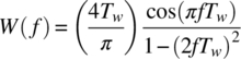
The spectrum shown in Figure 1.38a is based on computer simulation with N = 200 samples per window.

FIGURE 1.38 Cosine window spectrums.
1.11.3.2 Cosine‐Squared (Hanning) Window (k = 2)
The cosine‐squared window with k = 2 is referred to as a Hanning window [74]. Applying trigonometric identities, this window is expressed as
and the spectrum is shown in Figure 1.38b for N = 200 samples per window.
1.11.3.3 Cosine Window (k = 3 and 4)
Applying trigonometric identities, the cosine windows for k = 3 and 4 are expressed as
and
The spectrums for these two cases are shown in Figure 1.38c.
1.11.4 Temporal Raised‐Cosine (TRC) Window
The temporal raised‐cosine (TRC) window applies a cosine shaping function symmetrically about each end of the rectangular window function, rect(nΔt/Tw), as shown in Figure 1.39. In this case, the integer n corresponds to the samples N over the interval Tw such that N = Tw/Δt.

FIGURE 1.39 Temporal raised‐cosine window.
The TRC window is expressed as

where n′ = t/Tw = nΔt/Tw is the normalized sample index and α is a design parameter limited to 0 ≤ α ≤ 1. The TRC window is applied to the phase function of PSK‐modulated waveforms in Sections 4.2.8 and 4.4.3.9 to improve the waveform spectral containment while maintaining a constant signal amplitude; in this application α is referred to as the excess phase factor.
Letting m = f/Tw, the spectrum of the TRC amplitude window is evaluated as

1.11.4.1 Spectral Raised‐Cosine Window
The raised‐cosine window when applied in the frequency domain is referred to as the spectral RC (SRC) window and the parameter α is referred to as the excess bandwidth. With m = fTw, the SRC frequency response is expressed as

and upon letting n = t/Tw, the SRC impulse response is evaluated as

This response has indeterminate solutions of the form 0/0 at n = 0 and 1/(2α) that are evaluated as ![]() and
and

Using these results, (1.431) is plotted in Figure 1.40 for several values of the excess bandwidth factor. The SRRC window, associated with spectral shaping of a modulated symbol, is discussed in detail in Section 4.3.2. In this application the symbol duration is T = Tw and the transmitted symbol and demodulator‐matched filter spectrums have a square‐root RC, or simply root RC, frequency response of ![]() . The matched filter output results in the SRC impulse response shown in Figure 1.40 with symbol spacing corresponding to integer values of n that results in zero ISI ∀n ≠ 0. With an AWGN channel and optimum matched filter sampling the demodulator performance corresponds to maximum‐likelihood detection.
. The matched filter output results in the SRC impulse response shown in Figure 1.40 with symbol spacing corresponding to integer values of n that results in zero ISI ∀n ≠ 0. With an AWGN channel and optimum matched filter sampling the demodulator performance corresponds to maximum‐likelihood detection.

FIGURE 1.40 Impulse response of SRC window.
1.11.5 Blackman Window
The Blackman window uses three terms to provide more tapering of the window at the expense of a narrower time response and a wider noise bandwidth. The Blackman window is expressed as
where the phase function in (1.433) is expressed as

This definition of the phase function results in a symmetrical window for all values of N with indexing over ![]() as shown in Figure 1.41a for N = 21. The spectrum of the Blackman window corresponding to N = 200 samples per window is shown in Figure 1.41b.
as shown in Figure 1.41a for N = 21. The spectrum of the Blackman window corresponding to N = 200 samples per window is shown in Figure 1.41b.

FIGURE 1.41 Blackman window and spectrum.
1.11.6 Blackman–Harris Window
The Blackman–Harris window is expressed as
Harris [75] performed a gradient search on the coefficients ci to minimize spectral sidelobe level and the results are given in Table 1.16 for a three‐ and four‐term window.
TABLE 1.16 Blackman–Harris Window Coefficientsa
| Coefficient | 3‐Term 67 dB |
4‐Term 92 dB |
| c0 | 0.42323 | 0.35875 |
| c1 | 0.49755 | 0.48829 |
| c2 | 0.07922 | 0.14128 |
| c3 | 0.0 | 0.01168 |
aHarris [75]. Reproduced by permission of the IEEE.
The Blackman–Harris window, as formulated by Harris, divides the phase function by N that results in an asymmetrical window. To provide a symmetrical window for all N, the phase function ϕn is divided by N − 1 and expressed as

The spectrum of the 4‐Term 92 dB Blackman–Harris window is shown in Figure 1.42 for N = 200 samples per symbol and L = 40 samples in the bandwidth 1/Tw Hz.

FIGURE 1.42 Blackman–Harris window spectrum (N = 200, 92 dB, 4‐Term).
The coefficients for the Blackman–Harris function, as given in Table 1.16, do not result in window values of zero for the first and last sample resulting in a window pedestal of 6 × 10⁻⁵; this is a direct result of the coefficients not summing to zero at the window edges. The pedestal plays a critical role in the control of the sidelobes and noise bandwidth and windows with more dramatic pedestals are examined in the following sections.
1.11.7 Hamming Window
The Hamming window is expressed as
where the phase function ϕn is expressed as
The window is shown in Figure 1.43a with indexing over the range 0 ≤ n ≤ N − 1 and the spectrum is shown in Figure 1.43b.

FIGURE 1.43 Hamming window and spectrum.
1.11.8 Kaiser (Kaiser–Bessel) Window
The Kaiser window, also referred to as the Kaiser–Bessel window, is expressed as

where Io(x) is the modified Bessel function of order zero and β is the time‐bandwidth product equal to TwB where Tw is the window duration and B is the corresponding baseband bandwidth. The Kaiser window is shown in Figure 1.44a, using N = 51 samples per window, as a symmetrical window for β = 2, 3, and 4; the range −N/2 ≤ n ≤ N/2 corresponds to –Tw/2 ≤ t ≤ Tw/2. The corresponding spectrum of the Kaiser window is shown in Figure 1.44b.

FIGURE 1.44 Kaiser windows and spectrums (β = 2, 3, and 4).
1.12 MATRICES, VECTORS, AND RELATED OPERATIONS
A matrix is a convenient way to describe complicated linear systems and is used extensively in the analysis of control systems. For example, a large linear system is generally described in terms of the inputs xj, outputs yi, and the system coefficients aij as

and using matrix and vector notations (1.440) is described as

where the 1 by n inputs xj, and the 1 by m outputs yi are described by vectors and the coefficients aij are described by the m by n matrix. The notation of an m by n matrix refers, respectively, to the number of rows and columns of the matrix. The linear system may include time‐varying inputs, outputs, and coefficients as found in control systems and time‐varying parameter estimation and tracking applications. The following descriptions of matrices and vectors are introductory and targeted to the description of adaptive systems in Chapter 12. More in‐depth discussions on the subject and applications are given by Derusso, Roy, and Close [77], Haykin [78], Sage and White [79], and Gelb [80].
1.12.1 Definitions and Types of Matrices
- A m × n matrix A contains m rows and n columns of elements aij and is denoted as(1.442)

- A diagonal matrix (Λ) is a m × m square matrix with aij = 0: i ≠ j, otherwise, the elements on the principal diagonal are identified as aii with Λ = diag(aii) ∀ i.
- The unit matrix (I) is similar to the diagonal matrix with aij = 0: i ≠ j, and aii. = 1.
- A null matrix or zero matrix (O) is a matrix for which all of the elements are zero.
- A symmetric matrix is a square matrix of real elements if A = AT, that is, aji = aij ∀ i,j.
- A skew matrix is a square matrix of real elements if A = −AT, that is, aij = −aji ∀ i,j.
- A nonsingular matrix A has an inverse A−1.
- A complex matrix is denoted as à and has complex elements
 where acij and asij denote the respective real and imaginary values of the complex elements. Conjugation the complex matrix is denoted as Ã* with elements
  .
.
The transposition of the matrix interchanges the row and columns and is denoted with the superscript T. For example, the transpose of the matrix A is the n × m matrix denoted as

The Hermitian matrix is a complex matrix with the elements below the principal diagonal equal to the complex conjugate of the those about the principal diagonal; satisfying the conditions (A*)T = A+ = AH where the superscripts + and H denote the complex conjugate transposition. The superscript + generally denotes complex transposition and H is used to emphasize the Hermitian complex transposition.
The order, or rank, of an (m × n) matrix is denoted as m‐by‐n and the order, or rank, of the square (m × m) matrix is denoted as m.
1.12.2 The Determinant and Matrix Inverse
The determinant [81] of an m × m square matrix A is denoted as |A| and defined in terms of the cofactors, Aij, of A as

The cofactors are defined as
where Mij is the determinant of the minor matrix of the element aij. The ![]() minor matrix of aij is the matrix formed by the m′ rows and columns of A excluding the row and column containing aij. For example, considering the 4 × 4 square matrix A, the 3 × 3 minor matrix A′ of the element a32, and the determinant M32 are expressed in (1.446) as
minor matrix of aij is the matrix formed by the m′ rows and columns of A excluding the row and column containing aij. For example, considering the 4 × 4 square matrix A, the 3 × 3 minor matrix A′ of the element a32, and the determinant M32 are expressed in (1.446) as

Therefore, using (1.446), the cofactor A32 is evaluated as A32 = (−1)5M32. Following the evaluation of the remaining ![]() cofactors Ai,2: i = 1,2,4 or the cofactors A3j: j = 1,3,4, the determinant |A| is evaluated using, respectively, the first or second equality in (1.444).
cofactors Ai,2: i = 1,2,4 or the cofactors A3j: j = 1,3,4, the determinant |A| is evaluated using, respectively, the first or second equality in (1.444).
For square matrices of order ≤ 3, the determinant can be computed in terms of the elements aij as expressed, for example, in the 3 × 3 matrix described in (1.447). In this example, the determinant is formed by summing the n = 3 products of the elements parallel to the principal diagonal elements (a11,a22,a33) and subtracting the n = 3 products of the elements parallel to the diagonal elements (a13,a22,a31). The three positive products are indicated by solid arrows pointing to the diagonal elements parallel to the principal diagonal and the three negative products are indicated by dashed arrows pointing to the diagonal elements parallel to the complement of the principal diagonal. In both cases, the elements below the diagonals are wrapped around to form the three element products. In general, this procedure does not give the correct results for orders > 3.

Determinants are defined only for square matrices and if |A| = 0 the matrix A is referred to as a singular matrix, otherwise, A is nonsingular. The inverse of a nonsingular n × n matrix A, with elements aij, is expressed as

where the matrix [Aji] is defined as the adjoint of the matrix A. Considering the n × n matrix of cofactors [Aij] of the matrix A, with the cofactor of each element aij evaluated using (1.445), the adjoint matrix is the transpose of the matrix [Aij] so that
Premultiplication of A−1 by A results in the unit matrix, that is, AA−1 = I
1.12.3 Definition and Types of Vectors
A vector is an m × 1 column matrix with elements ai and is denoted as

A complex vector is denoted as ã with complex elements ![]() where ac and as denote the real and imaginary values of the complex element. The transposition of the matrix a is the 1 × m complex row vector aT. Conjugation and conjugate transposition are denoted by the respective superscripts * and +.
where ac and as denote the real and imaginary values of the complex element. The transposition of the matrix a is the 1 × m complex row vector aT. Conjugation and conjugate transposition are denoted by the respective superscripts * and +.
1.12.4 Matrix and Vector Operations
- Addition of two matrices of the same order (m × n) is C = A + B : The elements of C are cij = aij + bij
- Multiplication of the two matrices must conform to the following rule: [m × n][ n × m′] = [m × m′] where the inner dimension n must be identical.
- y = Ax : Matrix postmultiplication by a vector results in a [m × n][n × 1] = [m × 1] vector
- The element multiplication is

- y = xTA : Matrix premultiplication by a vector results in a [1 × n][n × m] = [1 × m] vector.
- The element multiplication is

- C = AB : Matrix multiplication results in a
 matrix
 - The element multiplication is

- In general, multiplication is not communicative AB ≠ BA
- A(BC) = (AB)C : Associative
- A(B + C) = AB + AC : Distributive
- Multiplication by diagonal matrix D
- C = AD : Postmultiplication of a real (m × m) matrix A by D results in a diagonal matrix C with the diagonal element of A scaled by those of D; the elements of C are cij = aijdjj : i,j = 1, …, m
- C = DA : Premultiplication of a real (m × m) matrix A by D results in the same diagonal matrix C; the elements of C are cij = diiaij : i,j = 1, …, m. In this case multiplication is communicative.
- Multiplication by unit matrix I
- IA = A : Multiplication of a (m × m) matrix A by I does not alter the matrix A.
- IA = AI : Multiplication by I is communicative.
- Transposition of AB
- C = (AB)T = ATBT
- Scalar, or inner, product of two (m × 1) complex vectors
 and ỹ
and ỹ  are complex values and
- Scalar product of two (m × 1) real vectors x and y
 is a real scalar value and
- Orthogonality of two vectors is defined if their scalar product is zero.
- Length of a complex vector
 is defined as magnitude, denoted as ||
 ||, of the inner product(1.451)
- Outer, or dyadic, product of two (m × 1) and (1 × n) complex vectors
 and ỹ forms an (m × n) complex matrix
  with elements
  . The autocorrelation matrix of a complex vector is computed as the outer product.
 - Differentiation of Complex Matrices: Differentiation of a complex matrix Ã(t) results in the complex matrix
 with elements evaluated as
  . The differentiation of sums and products of matrices is evaluated as(1.452)
 (1.453)
- Differentiation of a complex vector follows by considering the vector as a single column matrix. Therefore, differentiation of real matrices and vectors is identical with aij = 0.
- Differentiation of quadratic transformation with the matrix
 expressed as(1.454)
where the elements of the (m × m) complex matrix Ã(t) and the complex (m × 1) vector
 are functions of t. The derivative of
  is evaluated as(1.455)
- For a real matrix A(t) and vector x(t), the matrix Q(t) is symmetric and the derivative of the quadratic function Q(t) simplifies to(1.456)

- Bilinear transformation with the real (m × m) matrix B(t), expressed in terms of the (m × 1) real vectors x(t) and y(t), is evaluated as
- Differentiation of B(t) with respect to t is evaluated as(1.458)

1.12.5 The Quadratic Transformation
The quadratic matrix Q is similar to the bilinear matrix, expressed in (1.457), with the vector y = x. The following description is based on the (n × n) correlation matrix49
where ũ is an (n,1) complex vector of arbitrary data and ũH is the complex conjugate transpose50 of ũ. The n columns of the matrix Q represent the (n,1) characteristic vectors of the correlation matrix R that is transformed to the diagonal matrix Λ as
The diagonal elements of Λ are the characteristic values51 of the matrix R.
The derivation of (1.460) follows the work of Haykin [82] and is based on the linear transformation of the (n,1) complex vector ![]() to the vector
to the vector ![]() using the transformation
using the transformation
where λ is a constant. Equation (1.461) can be expressed as ![]() which has nontrivial solutions with
which has nontrivial solutions with ![]() ≠ 0, iff the determinant of R − λI is zero, that is,
≠ 0, iff the determinant of R − λI is zero, that is,
Equation (1.462) is the characteristic equation of the matrix R and has n solutions corresponding to the λi characteristic values or roots of (1.462). In general, the characteristic values are distinct; however, for the correlation matrix R, with the complex vector ũ based on samples of a discrete‐time weakly stationary stochastic process, the mean‐square value of the scalar ![]() is evaluated as
is evaluated as
Equation (1.463) corresponds to a nonnegative definite quadratic form and Haykin points out that the equality condition rarely applies in practice so that (1.463) is almost always positive definite.52 Consequently, in these cases, characteristic values are real with and λi > 0 ∀ i and, for the weakly stationary stochastic process, the characteristic values are equal with λi = σ2 ∀ i.
Referring to (1.461), the n solutions to the characteristic equation are determined using
where ![]() are the characteristic vectors corresponding to the characteristic values λi. Based on the correlation matrix R, it can be shown [83] that the characteristic values are all real and nonnegative and the characteristic vectors are linearly independent and orthogonal to each other. A corollary to the proof of independence is that when the characteristic value is multiplied by a scalar constant the characteristic vectors remain independent and orthogonal. This allows for the independent scaling of all characteristic values so that
are the characteristic vectors corresponding to the characteristic values λi. Based on the correlation matrix R, it can be shown [83] that the characteristic values are all real and nonnegative and the characteristic vectors are linearly independent and orthogonal to each other. A corollary to the proof of independence is that when the characteristic value is multiplied by a scalar constant the characteristic vectors remain independent and orthogonal. This allows for the independent scaling of all characteristic values so that

resulting in an orthonormal set of characteristic vectors satisfying (1.464). Recognizing that the matrix Q is a column of characteristic vectors with ![]() and Λ is a diagonal matrix of characteristic values
and Λ is a diagonal matrix of characteristic values ![]() , (1.464) is expressed as
, (1.464) is expressed as
and the orthonormal matrix Q satisfies the relationship QHQ = I, therefore, QH = Q−1 and premultiplying both sides of (1.466) by QH results in (1.460) as stated. Also, by postmultiplying both sides of (1.466) the correlation matrix is expressed as

Haykin states that there is no best way to compute the characteristic values and suggest that the use of the characteristic equation should be avoided except for the simple case involving the 2 × 2 matrix. However, a number of authors [77, 78, 84–89] describe computationally efficient methods for computing the characteristic values.
Consider the quadratic form ![]() discussed in Section 12.3, where
discussed in Section 12.3, where ![]() is a (m × 1) complex vector with elements
is a (m × 1) complex vector with elements ![]() and R=
and R= ![]() is a (m × m) Hermitian matrix with elements
is a (m × m) Hermitian matrix with elements ![]() : i ≠ j corresponding to the autocorrelation matrix of the (m × 1) complex vector
: i ≠ j corresponding to the autocorrelation matrix of the (m × 1) complex vector ![]() . The following derivatives with respect to the complex vector
. The following derivatives with respect to the complex vector ![]() are evaluated as:
are evaluated as:
and
where ![]() is a (m × 1) complex vector. The solutions to the derivative of the quadratic form with respect to the vector w are used in Chapter 12 in the analysis of adaptive systems. The proofs of (1.468), (1.469), and (1.470) are given by Haykin [78].
is a (m × 1) complex vector. The solutions to the derivative of the quadratic form with respect to the vector w are used in Chapter 12 in the analysis of adaptive systems. The proofs of (1.468), (1.469), and (1.470) are given by Haykin [78].
1.13 OFTEN USED MATHEMATICAL PROCEDURES
This section outlines the processing and formulas encountered in several of the chapters throughout this book.
1.13.1 Prime Factorization and Determination of Greatest Common Factor and Least Common Multiple
Prime factors are used in various coding applications where polynomials are used as code generators. The greatest common factor (GCF) and least common multiple (LCM) are often used where signal processing sample‐rate changes are required to improve performance or reduce processing complexity. They are also used in the implementation of mixed radix fast Fourier transforms. An integer p is prime if p ≠ ±1 and the only divisors are ±p and ±1. The procedures involved in determining the prime factors of a number and the GCF and LCM between two or more numbers are simply given by way of the following examples. The algorithms are easy to generalize and implement in a computer program.
1.13.1.1 Prime Factors of Two Numbers
The following examples, presented in Table 1.17, demonstrate the procedure for determining the prime factors of the numbers 120 and 200. The results are used in the following two examples to determine the GCF and LCM. The prime factors of a number are determined, starting with repeated division of the number by 2.
TABLE 1.17 Example of Prime Factorization
| Using 120 | Using 200 |
| 120 ÷ 2 = 60 | 200 ÷ 2 = 100 |
| 60 ÷ 2 = 30 | 100 ÷ 2 = 50 |
| 30 ÷ 2 = 15 | 50 ÷ 2 = 25 |
| 15 ÷ 3 = 5 | 25 ÷ 5 = 5 |
| 5 ÷ 5 = 1 | 5 ÷ 5 = 1 |
| The prime factors are: | |
| 2 × 2 × 2 × 3 × 5 | 2 × 2 × 2 × 5 × 5 |
1.13.1.2 Determination of the Greatest Common Factor
This example outlines the procedures in determining the GCF of the two numbers 120 and 200 using the prime factors listed in Table 1.17; inclusion of more than more than two numbers is straightforward. The GCF is also referred to as the greatest common divisor (GCD). The GCF (or GCD) between 120 and 200 is determined as the product of the prime factors taken the minimum number of times that they occurred in any one of the prime factorizations, that is,
1.13.1.3 Determination of the Least Common Multiple
This example outlines the procedures in determining the LCM between 120 and 200. In this case, the LCM is determined as the product of the prime factors taken the maximum number of times that they occurred in any one of the prime factorizations, that is,
1.13.2 Newton’s Method
A transcendental equation involves trigonometric, exponential, logarithmic, and other functions that do not lend themselves to solutions by algebraic means. Newton’s method [90] of solving transcendental equations is used extensively in arriving at solutions to problems characterized by nonalgebraic equations. The method provides a rapid and accurate solution to determine the value of functions having the form f(x) = h(x), by finding the solution of the auxiliary function g(x) = f(x) – h(x) = 0. The solution begins by starting with an estimate ![]() of the solution and performing iterative updates to the estimate, described as
of the solution and performing iterative updates to the estimate, described as

where g′(xi) = ∂g(xi)/∂xi. The evaluation is terminated when ![]() where ε is an acceptable error in the solution and the corresponding xi+1 is the desired value of x satisfying f(x) ≅ h(x).
where ε is an acceptable error in the solution and the corresponding xi+1 is the desired value of x satisfying f(x) ≅ h(x).
1.13.3 Standard Deviation of Sampled Population
When a finite number of samples n comprises the entire population, the standard deviation is computed as

where the summation is over the entire population. However, when the samples n are a subset of the entire population, the standard deviation is computed as

where the summations are over the sample size n of the subset.
1.13.4 Solution to the Indeterminate Form 0/0
The frequently encountered functional form

evaluated at x = a often results in the indeterminate form 0/0 resulting from f(a) = g(a) = 0. Application of L’Hospital’s rule of repeated differentiation of f(x) and g(x) and evaluating the result as

often leads to a solution for n = 1 or 2. Solutions to other indeterminate forms involving ∞/∞, 0*∞, ∞−∞, 00, ∞0, 0∞, and 1∞ may also be found using similar techniques [90, 91].
1.14 OFTEN USED MATHEMATICAL RELATIONSHIPS
In this section a number of mathematical relationships are listed as found in various mathematical handbooks. The references frequently referred to are as follows: Burington [92], Korn and Korn [93], Milton and Stegun [94], and Gradshteyn and Ryzhik [46].
1.14.1 Finite and Infinite Sums


1.14.2 Binomial Theorem and Coefficients


1.14.3 Trigonometric Identities


1.14.4 Differentiation and Integration Rules
The notations u and v are functions of x


 ;
; 
 ;
; 
 ;
; 
 ;
; 
 ;
; 
 ;
; 
 ;
; 
 ;
; 
 : integration by parts with u = f(x) and dv = g(x)dx


1.14.5 Inequalities


 bn > 0; equality holds iff bn = an
 Equality holds for c = constant > 0 iff an= c bn
 Equality holds for c = constant > 0 iff f(x) = c g(x).
1.14.6 Relationships between Complex Numbers
For ![]() and
and ![]()

 ;
; 


1.14.7 Miscellaneous Relationships [94]


 [95]
[95] [95]
[95]


 53
53
Example: for b = 3: a = …−4 −3 −2 −1 0 1 2 3 4 …
r = …−1 0 –2 −1 0 1 2 0 1 …
 *
*
Example: for b = 3: a = …−4 −3 −2 −1 0 1 2 3 4 …
r = … 2 0 1 2 0 1 2 0 1 …
 *
*- The solutions to the quadratic equation
 is
is 
- Completing the square of:

- Completing the square of:

ACRONYMS
- ACI
- Adjacent channel interference
- ACK
- Acknowledgment (protocol)
- AFSCN
- U.S. Air Force Satellite Control Network
- AM
- Amplitude modulation
- ARQ
- Automatic repeat request
- AWGN
- Additive white Gaussian noise
- BPSK
- Binary phase shift keying
- BT
- Time bandwidth (product, low pass)
- CFAR
- Constant false‐alarm rate
- CRC
- Cyclic redundancy check (code)
- DC
- Direct current
- DFT
- Discrete Fourier transform
- DSB
- Double sideband
- DSSS
- Direct‐sequence spread‐spectrum (waveform)
- EHF
- Extremely high frequency
- ELF
- Extremely low frequency
- FFT
- Fast Fourier transform
- FM
- Frequency modulation
- FSK
- Frequency shift keying
- GCD
- Greatest common divisor
- GCF
- Greatest common factor
- HF
- High frequency
- I/Q
- In‐phase and quadrature (channels or rails)
- IDFT
- Inverse discrete Fourier transform
- IF
- Intermediate frequency
- IFFT
- Inverse Fast Fourier transform
- ISI
- Intersymbol interference
- LCM
- Least common multiple
- LF
- Low frequency
- LLR
- Log‐likelihood ratio
- LR
- Likelihood ratio
- MAP
- Maximum a posteriori
- MF
- Medium frequency
- ML
- Maximum likelihood
- MMSE
- Minimum mean‐square error
- MS
- Mean square
- MSK
- Minimum shift keying
- NAK
- Negative acknowledgment (protocol)
- OQPSK
- Offset quadrature phase shift keying
- PM
- Phase modulation
- PN
- Pseudo‐noise (sequence)
- PSD
- Power spectral density
- PSK
- Phase shift keying
- QAM
- Quadrature amplitude modulation
- QPSK
- Quadrature phase shift keying
- RC
- Raised‐cosine
- RQ
- Repeat request
- RRC
- Root‐raised‐cosine (temporal)
- RSS
- Root‐sum‐square
- SHF
- Super high frequency
- SLF
- Super low frequency
- SRC
- Spectral raised‐cosine
- SRRC
- Spectral root‐raised‐cosine
- SS
- Spread‐spectrum
- TRC
- Temporal raised‐cosine
- UHF
- Ultra‐high frequency
- ULF
- Ultra‐low frequency
- VLF
- Very low frequency
- WSS
- Wide‐sense stationary
- WT
- Time bandwidth (product, bandpass)
PROBLEMS
- Show that the amplitude‐modulated waveform given by (1.2), when heterodyned by a receiver local oscillator that is phase locked to the received carrier angular frequency ωc, recovers the modulation function
 , except for a factor of 1/2.
Hint: Mix (1.2) with sin(ωct+ϕ) and show that ϕ must be zero.
- Show that the real signal given by (1.13) is a form of suppressed carrier modulation. Under what conditions of M(t) and ϕ(t) + ψ(t) does (1.13) reduce to the form of the suppressed carrier modulation given by (1.12)? What can be said about the information capacity between the suppressed carrier modulations given by (1.12) and (1.13)?
- Compute the Hilbert transform of
 and
and  .
. - Given that the bandwidth of the modulation function A(t) satisfies the condition B << fc, compute the Hilbert transform of
 .
. - Show that the Fourier coefficients Cn and C−n, expressed in (1.30), form complex conjugate pairs when f(t) is real.
- Show that the real‐valued function f(t) can be expressed in terms of the Fourier series real coefficient Co = αo and the complex coefficients Cn = αn + jβn: 1 ≤ n ≤ ∞ aswhere

 and
and  . Note: This solution is based on Problem 5.
 - Show that the finite summation
 is equal to the second equality in (1.52).
Hint: Expand the summation and combine the exponential terms to yield a series involving cos(nωoT) terms and then evaluate the closed form of the corresponding trigonometric series as identified in Section 1.14.1 Identity No. 12.
- With ωo = 2π/T show that the integral
 is equal to unity as N → ∞.
 - Referring to Figure 1.7 and using ωo = 2π/T, show that the maximum value of (1.52) is (2N + 1)/T and that the closest zero or null removed from a maximum occurs at t = nT ± T/(2N + 1): |n| = 0,1,….
- Consider a radix‐2, N‐point, pipeline FFT with the output sampled at intervals of T = NsTs seconds, where Ns is the number of samples per symbol. If the sequential input samples are simply passed through the FFT delay elements with the complex multiplications and additions only performed at the output sampling instants: (A) determine the percentage of complex multiplies relative to the pipeline FFT sampled every Ts seconds. Examine the result as a function of increasing Ns with 1 ≤ Ns ≤ 32 and N ≥ Ns; (B) determine the minimum number of complex multiplications when 100 % zero padding is used for frequency estimation and tracking and discuss the pipeline FFT sampling requirements.
- Compute the second moment, E[X2], of the Gaussian random variable X with mean m and variance σ2.
- Referring to (1.165) compute
 for the conditional Gaussian pdf, expressed by the second equality of (1.168), with
  and
and  . Express the result in terms of the expectations as
  and express C1, C2, and C3 in terms of the parameters
  .
.
Using
 ,
,  , and
, and  evaluate
  with m1 = m2 = 0.
 - Repeat Problem 12 using (1.172) and show thatwhen x1 and x2 are zero‐mean Gaussian random variables.

- In the transformation from fX(x) to fZ(z), discussed in Section 1.5.4.1, show that the inverse relationship in (1.188) applies for the function z = ax2.
Part B: Express fZ(z) using (1.186) or (1.187).
Part C: Express fZ(z) when the pdf of fX(x) is Gaussian with mean value m and variance σ2. Plot or sketch your expression fZ(z) as a function of z.
Note: eλ + e−λ = 2cosh(λ).
Part D: Express fZ(z) when m = 0 in Part C and plot or sketch as a function of z.
- Given the statistically independent ordered random variables {X1, X2, …, Xn} such that a ≤ X1<X2<⋯<Xn ≤ b and characterized by the uniformly distributed pdf
 : ∀i,
: ∀i,  with the corresponding cdf expressed as
  . Show that
 with
with  .
.
Hint: Start with
 with
with  and note that
  .
. - For the transformation in Section 1.5.5, evaluate the Jacobian in (1.211) using the phase angle expressed as θ = tan−1(xs/xc).
Hint: use g11(xc,xs) = g12(xc,xs) =
 and g21(xc,xs) = g22(xc,xs) = tan−1(xs/xc).
 - Given the joint pdf fX,Y(x,y), expressed in (1.166), compute the marginal pdf MX(x).
Hint: Complete the square using:
 .
. - Given the pdf fX,(x), perform the following:
- Compute the pdf fY,(y) under the condition y = |x|. Note that fY,(y) = 0 for y < 0.
- Determine and sketch fY,(y) when fX,(x) is described by the normal distribution N(mx,σx)
- Repeat Part B with mx = 0
- Show that the limiting form of the Ricean distribution, expressed by (1.222), corresponds to the Rayleigh distribution as A → 0. Refer to Table 1.8.
Hint: Use the ascending series expression
 with
with  .
. - Show that the limiting form of the Ricean distribution, expressed by (1.222), corresponds to the Gaussian distribution as A → ∞. Refer to Table 1.8.
Hint: Use the asymptotic expansion of Io(z) for large arguments expressed asIo(z) ~
 with
with  .
.Recognize that as r → A the condition r = A results in the Gaussian distribution.
- Determine the marginal pdf of Y1 = min{X1, X2, …, Xn} given the joint pdf gY(y1, y2, …, yn) of the uniformly distributed ordered samples
 corresponding to
  .
.
Hint: Show that the cdfs in the descending order
 are expressed as
with
 and
and  .
.Also show that
 where
where  .
. - Show that the Nakagami‐m distribution is the same as the Rayleigh power distribution.
Hint: Use the transformation
 in the Rayleigh distribution.
 - Derive the expression for the characteristic function CX(v) for the Gaussian distribution fX(x) with mean value xo and variance σ2.
- Set up the integrations identifying the integration limits and ranges of the variable z for the evaluation of fZ(z) where the random variable Z is the summation of three (3) zero‐mean uniformly distributed random variables X between –a and a.
Hint: There are three unique ranges on z. The evaluation of the integrations is optional; however, the application of Mathsoft’s Mathcad® symbolic formula evaluation is an error‐free time saver.
- Using fZ(z) evaluated in Problem 24 for N = 3, compute the first and second moments of the random variable Z using (1.254) and compare the results with those in Table 24.
Hint: It is much easier and less prone to mistakes to use Mathsoft’s Mathcad symbolic formula evaluation.
- Show that the moments of the random variable X are determined from the characteristic function as expressed in (1.240).
Hint: Take the first derivative of CX(v) with respect to v and evaluate the result for v = 0; and observe that the resulting integral is E[x]. Repeat this procedure for additional derivatives of CX(v) and show that (1.240) follows.
- Plot the cdf of a zero‐mean Gaussian distribution with variances corresponding to the second moments in Table 1.6 for N = 3 and 4 and compare the results with the corresponding cdf’s in Figure 1.23; comment on the quality of the match in light of the central limit theorem. Repeat this exercise using the theoretical second moments from Table 1.7 for N = 3 and 4 and compare with the corresponding cdf’s in Figure 1.26.
- Show that equations (1.261) and (1.262) apply for λv <<1 as N increases in the respective summation of N iid distributions in Examples 1 and 2 of Section 1.5.6.1.
- The narrowband noise process n(t), given by (1.307), is expressed in terms of the baseband analytic noise ñ(t) asUsing this relationship, express the correlation function

 in terms of the individual correlation functions
  , Rññ(τ),
  and
and  . What are the required conditions on these correlation functions to satisfy the stationarity property of the narrowband process n(t)?
 - Express the individual correlation functions in Problem 29 in terms of the correlation functions Rcc(τ), Rcs(τ), Rsc(τ), and Rss(τ), where the baseband analytic noise is given by
 . Use these results and the conditions for stationarity found in Problem 29 to express Rnn(τ) in terms of the Rcc(τ) and Rsc(τ).
 - Referring to (1.315), that applies to the noise power out of a bandpass filter centered at the positive frequency fc. When the bandpass filter output is mixed to baseband, express the noise power out the baseband filter in terms of the bandwidth B and the one‐sided noise spectral density No.
- Given the noise input, expressed by (1.307), to a linear filter with impulse response h(t), show that the respective input and output of the correlation responses Rnn(τ) and
 are related by the convolutions
  . Using this result with Fourier transform pairs h(τ) ↔ H(f) and h*(−τ) ↔ H*(f), show the relationship between the input and output noise spectrums.
Hint: Using the convolution integral
 show that n′(t) has zero‐mean. Then from the correlation
and show that
 and, as the final step, form the correlation
and show that
 .
. - Derive the expression for the matched filter output signal‐to‐noise ratio when the additive noise is not white noise, that is, the noise power spectral density into the matched filter is
 .
. - Under the condition stated in Section 1.7.1 show that (1.332) is a wide‐sense stationary random process.
- Given the random process x(ti) = a where ti is a discrete‐time sample and a is a discrete random variable such that a = 1 with probability p and = −1 with probability q = 1 − p. Using (1.303) and (1.304) determine if x(ti) is ergodic.
- Show that the random process
 is wss if fc is constant and x(t) is a wss random process independent of the random variable ϕ uniformly distributed over the interval 0 to 2π. Also, express the PSD Sy(ω) in terms of the autocorrelation Rx(τ) and the PSD Sx(ω).
 - The risk for the mean‐square estimate is defined asShow that

 and results in the optimum estimate given by (1.356).
 - Determine if the MS and MAP estimates in the example of Section 1.9.1 are unbiased estimates. If not, what is the bias of the estimate? Also, evaluate the Cramér–Rao bound for the estimates and, using (1.366), determine if the estimates are efficient.
- Given that the received baseband signal amplitude is A volts, using the ML estimate, determine the following: Part 1, the variance
 of the estimation error of A given the baseband samples
  : i = 1, …, N where ni are iid Gaussian random variables characterized as N(0,σn), Part 2, show that the estimate âml(r) is efficient, Part 3 show the condition for which the estimate âml(r) is unbiased.
 - Repeat Problem 39 under the following condition: the baseband signal amplitude is Gaussian distributed with a priori pdf pa(A) characterized by N(A,σa).
- Using (1.384) determine the effective bandwidth (β) for the isosceles triangle shaped pulse with base equal to 2τ and peak amplitude of AN volts.
Hints: The solution to the integral
 is encountered with m = 2 and the double factorial [96] is defined as (2m + 1)!! = 1 × 3 × 5 … (2m + 1). The denominator in the expression for α2 is the signal energy E.
 - Determine the normalized effective bandwidth (βT) and the corresponding standard deviation (σTd) for the SRC and SRRC waveforms with 100% excess bandwidth, that is, α = 1.
- Determine the normalized effective bandwidth (βT) and the corresponding standard deviation (σTd) of the delay estimate for the SRC and SRRC waveforms with zero excess bandwidth, that is, α = 0.
- Determine the noise bandwidth for the SRRC and SRC frequency functions.
Note: the noise bandwidth is defined by (1.46).
- Using (1.387) determine the normalized effective time duration
 for the rectangular pulse Arect(t/T − 0.5).
REFERENCES
- 1. C.E. Shannon, “Communication in the Presence of Noise,” Proceedings of the IEEE, Vol. 86, Issue 2, pp. 447–457, February, 1998.
- 2. M. Abramowitz, I.A. Stegun, Handbook of Mathematical Functions with Formula, Graphs and Mathematical Tables, National Bureau of Standards, Applied Mathematical Series 55, Washington, DC, U.S. Government Printing Office, p. 361, June 1964.
- 3. R.A. Manske, “Computer Simulation of Narrowband Systems,” IEEE Transactions on Computers, Vol. C‐17, No. 4, pp. 301–308, April 1968.
- 4. E.C. Titchmarsh, The Theory of Functions, 2 ed., Oxford University Press, New York, 1939.
- 5. E.C. Titchmarsh, Introduction to the Theory of Fourier Integrals, 2 ed., Oxford University Press, New York, 1948.
- 6. W.B. Davenport, Jr., W.L. Root, An Introduction to the Theory of Random Signals and Noise, McGraw Hill Book Company, New York, 1958.
- 7. A. Papoulis, The Fourier Integral and Its Applications, pp. 9, 42–47, McGraw‐Hill Book Company, New York, 1987.
- 8. A. Papoulis, Probability, Random Variables and Stochastic Processes, McGraw‐Hill Book Company, New York, 1965.
- 9. A.V. Oppenheim, R.W. Schafer, Digital Signal Processing, Chapter 11, “Power Spectrum Estimation”, Prentice‐Hall, Inc., Englewood Cliffs, NJ, 1975.
- 10. M.S. Bartlett, An Introduction to Stochastic Processes with Special Reference to Methods and Applications, Cambridge University Press, New York, 1953.
- 11. B.P. Bogert, Guest Editor, “The Fast Fourier Transform and Its Application to Digital Filtering and Spectral Analysis,” Special Issue of the IEEE Transactions on Audio and Electroacoustics, Vol. AU‐15, No. 2, June 1967.
- 12. J.W. Cooley, P.A.W. Lewis, P.D. Welch, “The Finite Fourier Transform,” IEEE Transactions on Audio and Electroacoustics, Vol. AU‐17, No. 2, pp. 77–85, June 1969.
- 13. R.C. Singleton, “A Short Bibliography on the Fast Fourier Transform,” IEEE Transactions on Audio and Electroacoustics, Vol. AU‐17, No. 2, pp. 166–169, June 1969.
- 14. G.D. Bergland, “A Guided Tour of the Fast Fourier Transform,” IEEE Spectrum, Vol. 6, pp. 41–52, July 1969.
- 15. T.H. Glisson, C.I. Black, A.P. Sage, “The Digital Computation of Discrete Spectra Using the Fast Fourier Transform,” IEEE Transactions on Audio and Electroacoustics, Vol. AU‐18, No. 3, pp. 271–287, September 1970.
- 16. J.D. Merkel, “FFT Pruning,” IEEE Transactions on Audio and Electroacoustics, Vol. AU‐19, No. 4, pp. 305–311, September 1971.
- 17. P.D. Welch, “The Use of the Fast Fourier Transform for the Estimation of Power Spectra: A Method Based on Time Averaging over Short, Modified Periodograms,” IEEE Transactions on Audio and Electroacoustics, Vol. AU‐15, pp. 70–73, June 1967.
- 18. J.W. Cooley, J.W. Tukey, “An Algorithm for Machine Calculation of Complex Fourier Series,” Mathematical Computation, Vol. 9, No. 5, pp. 297–301, April 1965.
- 19. E.O. Brigham, R.E. Morrow, “The Fast Fourier Transform,” IEEE Spectrum, Vol. 4, No. 2, pp. 63–70, December 1967.
- 20. E.O. Brigham, The Fast Fourier Transform and Its Applications, Prentice‐Hall, Inc., Englewood Cliffs, NJ, 1988.
- 21. H.L. Groginsky, G.A. Works, “A Pipeline Fast Fourier Transform,” IEEE Transactions on Computers, Vol. C‐19, No. 11, pp. 1015–1019, November 1970.
- 22. A.V. Oppenheim, R.W. Schafer, Digital Signal Processing, pp. 542–554, Prentice‐Hall, Inc., Englewood Cliffs, NJ, 1975.
- 23. A.V. Oppenheim, R.W. Schafer, Digital Signal Processing, pp. 548–549, Prentice‐Hall, Inc., Englewood Cliffs, NJ, 1975.
- 24. P.M. Woodward, Probability and Information Theory, with Applications to Radar, Pergamon Press, London, 1960.
- 25. M. Abramowitz, I.A. Stegun, Handbook of Mathematical Functions with Formula, Graphs and Mathematical Tables, National Bureau of Standards, Applied Mathematical Series 55, Washington, DC, U.S. Government Printing Office, p. 231, June 1964.
- 26. P.F. Panter, Modulation, Noise, and Spectral Analysis Applied to Information Transmission, McGraw‐Hill Book Company, New York, 1965.
- 27. S. Goldman, Transformation calculus and Electrical Transients, Chapter 9, “Bessel Functions,” Prentice‐Hall, Inc., Englewood Cliffs, NJ, 1950.
- 28. H. Cramér, Mathematical Methods of Statistics, Princeton University Press, Princeton, NJ, 1974.
- 29. A. Leon‐Garcia, Probability and Random Processes for Electrical Engineering, Second Addition, Addison‐Wesley Publishing Company, Inc., New York, May 1994.
- 30. J.M. Wozencraft, I.M. Jacobs, Principles of Communication Engineering, John Wiley & Sons, Inc., New York, 1967.
- 31. H.D. Brunk, An Introduction to Mathematical Statistics, Blaisdell Publishing Company, Waltham, MA, 1965.
- 32. W. Feller, An Introduction to Probability Theory and Its Applications, John Wiley & Sons, Inc., New York, 1957.
- 33. A. Papoulis, Probability, Random Variables, and Stochastic Processes, p. 236, McGraw‐Hill Book Co., New York, 1965.
- 34. A. Papoulis, Probability, Random Variables, and Stochastic Processes, p. 176, McGraw‐Hill Book Co., New York, 1965.
- 35. A. Papoulis, Probability, Random Variables, and Stochastic Processes, pp. 207–209, McGraw‐Hill Book Co., New York, 1965.
- 36. W.B. Davenport, Jr., W.L. Root, An Introduction to the Theory of Random Signals and Noise, p. 149, McGraw Hill Book Co., New York, 1958.
- 37. A. Papoulis, Probability, Random Variables, and Stochastic Processes, p. 221, McGraw‐Hill Book Co., New York, 1965.
- 38. W.B. Davenport, Jr., W.L. Root, An Introduction to the Theory of Random Signals and Noise, pp. 33–35, McGraw Hill Book Co., New York, 1958.
- 39. A. Papoulis, Probability, Random Variables, and Stochastic Processes, pp. 126–127, McGraw‐Hill Book Co., New York, 1965.
- 40. N.A.J. Hastings, J.B. Peacock, Statistical Distributions: A Handbook for Students and Practitioners, A Halsted Press Book, John Wiley & Sons, Inc., New York, 1975.
- 41. W.B. Davenport, Jr., W.L. Root, An Introduction to the Theory of Random Signals and Noise, p. 165, McGraw Hill, New York, 1958.
- 42. W.B. Davenport, Jr., W.L. Root, An Introduction to the Theory of Random Signals and Noise, p. 166, McGraw Hill, New York, 1958.
- 43. M. Abramowitz, I.A. Stegun, Handbook of Mathematical Functions with Formulas, Graphs, and Mathematical Tables, National Bureau of Standards, Applied Mathematics Series No. 55, U.S. Government Printing Office, Washington, DC, p. 376, Integral 9.6.16, June 1964.
- 44. W.B. Davenport, Jr., W.L. Root, An Introduction to the Theory of Random Signals and Noise, pp. 165–167, McGraw Hill Book Co., New York, 1958.
- 45. J.C. Hancock, An Introduction to the Principles of Communication Theory, McGraw‐Hill Book Co., New York, 1961.
- 46. I.S. Gradshteyn, I.M. Ryzhik, Table of Integrals, Series, and Products, Corrected and Enlarged Edition, Academic Press, Inc., New York, 1980.
- 47. G.A. Campbell, R.M. Foster, Fourier Integrals for Practical Applications, Fourth Printing, D. Van Norstrand Company, Inc., New York, 1948.
- 48. H. Urkowitz, “Energy Detection of Unknown Deterministic Signals,” Proceeding of the IEEE, Vol. 55, No. 4, pp. 523–531, April 1967.
- 49. M. Nakagami, “The m‐distribution—A general formula for Intensity Distribution of Rapid Fading,” W.C. Hoffman, Editor, Statistical Methods in Radio Wave Propagation, pp. 3–36, Pergamon Press, New York, 1960.
- 50. M.G. Kendall, A. Stuart, The Advanced Theory of Statistics, Vol. I, II, Hafner Publishing Company, New York, 1958, 1961 and Advanced Theory of Statistics, Vol. III, Hafner Press, New York, 1982.
- 51. H.A. David, H.N. Nagaraja, Order Statistics, 3rd Addition, John Wiley & Sons, Hoboken, NJ, 2003.
- 52. B.W. Lindgren, Statistical Theory, The Macmillan Company, New York, 1962.
- 53. R.C. Borgioli, “Fast Fourier Transform Correlation versus Direct Discrete Time Correlation,” Proceeding of the IEEE, Vol. 56, No. 9, pp. 1602–1604, September, 1968.
- 54. E.O. Brigham, Editor, The Fast Fourier Transform and its Applications, Chapter 10, “FFT Convolution and Correlation,” Prentice‐Hall, Englewood Cliffs, NJ, 1988.
- 55. A. Papoulis, Editor, Probability, Random Variables, and Stochastic Processes, Chapter 9, “Stochastic Processes: General Concepts,” McGraw‐Hill Book Co., New York, 1965.
- 56. W.B. Davenport, Jr., W.L. Root, An Introduction to the Theory of Random Signals and Noise, pp. 38–42, 66–71, McGraw Hill Book Co., New York, 1958.
- 57. A. Papoulis, Probability, Random Variables, and Stochastic Processes, pp. 323–332, McGraw‐Hill Book Co., New York, 1965.
- 58. A. Papoulis, Editor, Probability, Random Variables, and Stochastic Processes, Chapter 10, “Stochastic Processes: Correlation and Power Spectrum of Stationary Processes,” McGraw‐Hill Book Co., New York, 1965.
- 59. D.O. North, “Analysis of the Factors Which Determine Signal/Noise Discrimination in Radar,” Radio Corporation of America (RCA), Technical Report PTR‐6‐C, June, 1943; reprinted in Proceeding of the IRE, Vol. 51, pp. 1016–1028, July 1963.
- 60. G.L. Turin, “An Introduction to the Matched Filter,” IRE Transactions on Information Theory, Vol. 6, No. 3, pp. 311–329, June 1960.
- 61. M.L. Skolnik, Introduction to Radar Systems, McGraw‐Hill Book Company, Inc., New York, 1962.
- 62. D. Slepian, “Estimation of Signal Parameters in the Presence of Noise,” IRE Transactions on Information Theory, Vol. PGIT‐3, No. 4, pp. 68–89, March 1954.
- 63. P.M. Woodward, I.L. Davies, “Information Theory and Inverse Probability in Telecommunication,” Proceedings of the IEE, Vol. 99, Part III, pp. 37–44, March 1952.
- 64. H. Cramér, Mathematical Methods of Statistics, Chapter 32, “Classification of Estimates,” Princeton University Press, Princeton, NJ, 1974.
- 65. C.R. Rao, “Information and Accuracy Attainable in the Estimation of Statistical Parameters,” Bulletin Calcutta Mathematical Society, Vol. 37, pp. 81–91, 1945.
- 66. H.L. Van Trees, Detection, Estimation, and Modulation Theory: Part I, John Wiley & Sons, New York, 1968.
- 67. C.E. Cook, M. Bernfeld, Radar Signals: An Introduction to Theory and Application, Academic Press, New York, 1967.
- 68. L. Kleinrock, Queueing Systems, Volume I: Theory, John Wiley & Sons, New York, 1975.
- 69. D. Gabor, “The Theory of Communication,” Journal of the IEE, Vol. 93, Part III, pp. 429–441, 1946.
- 70. R. Manasse, “Range and Velocity Accuracy from Radar Measurements,” MIT Lincoln Laboratory, Lexington, MA, February, 1955. (This unpublished internal report is not generally available.)
- 71. M.L. Skolnik, Introduction to Radar Systems, pp. 467–469, McGraw‐Hill Book Co., Inc., New York, 1962.
- 72. F. Halsall, Data Communications, Computer, Networks and Open Systems, Fourth Edition, Addison‐Wesley Publishing Company, Harlow, UK, 1996.
- 73. C. Fujiwara, K. Yamashita, M. Kasahara, T. Namekawa, “General Analyses Go‐Back‐N ARQ System,” Electronics and Communications in Japan, Vol. J59‐A, No. 4, pp. 24–31, 1975.
- 74. A.V. Oppenheim, R.W. Schafer, Digital Signal Processing, Chapter 5, “Digital Filter Design Techniques,” Prentice‐Hall, Inc., Englewood Cliffs, NJ, 1975.
- 75. F.J. Harris, “On the Use of Windows for Harmonic Analysis with the Discrete Fourier Transform,” Proceeding of the IEEE, Vol. 66, No. 1, pp. 51–83, January 1978.
- 76. L.S. Metzger, D.M. Boroson, J.J. Uhran, Jr., I. Kalet, “Receiver Windows for FDM MFSK Signals,” IEEE Transactions on Communications, Vol. 27, No. 10, pp. 1519–1527, October 1979.
- 77. P.M. Derusso, R.J. Roy, C.M. Close, State Variables for Engineers, John Wiley & Sons, Inc., New York, 1965.
- 78. S. Haykin, Adaptive Filter Theory, Prentice‐Hall, Englewood Cliffs, NJ, 1986.
- 79. A.P. Sage, C.C. White, III, Optimum System Control, 2nd Edition, Prentice‐Hall, Inc., Englewood Cliffs, NJ, 1977.
- 80. A. Gelb, Editor, Applied Optimum Estimation, The M.I.T. Press, Massachusetts Institute of Technology, Cambridge, MA, 1974.
- 81. C.R. Wylie, Jr., Advanced Engineering Mathematics, McGraw‐Hill Book Company, Inc., New York, 1960.
- 82. S. Haykin, Adaptive Filter Theory, Chapter 2, “Stationary Discrete‐Time Stochastic Processes,” Prentice‐Hall, Englewood Cliffs, NJ, 1986.
- 83. S. Haykin, Adaptive Filter Theory, pp. 54–56, Prentice‐Hall, Englewood Cliffs, NJ, 1986.
- 84. G.W. Stewart, Introduction to Matrix Computations, Academic Press, New York, 1973.
- 85. J.S. Frame, “Matrix Functions and Applications, Part I – Matrix Operations and Generalized Inverses,” IEEE Spectrum, Vol. 1, No. 3, pp. 209–220, March 1964.
- 86. J.S. Frame, “Matrix Functions and Applications, Part II – Functions of a Matrix,” IEEE Spectrum, Vol. 1, No. 4, pp. 102–110, April 1964.
- 87. J.S. Frame, H.E. Koenig, “Matrix Functions and Applications, Part III – Applications of Matrices to Systems Analysis, a Matrix,” IEEE Spectrum, Vol. 1, No. 5, pp. 100–109, May 1964.
- 88. J.S. Frame, “Matrix Functions and Applications, Part IV – Matrix Functions and Constituent Matrices,” IEEE Spectrum, Vol. 1, No. 6, pp. 123–131, June 1964.
- 89. J.S. Frame, “Matrix Functions and Applications, Part V – Similarity Reductions by Rational or Orthogonal Matrices,” IEEE Spectrum, Vol. 1, No. 7, pp. 103–109, June 1964.
- 90. L.L. Smail, Calculus, Appleton‐Century‐Crofts, Inc., New York, 1949.
- 91. O.W. Eshbach, Handbook of Engineering Fundamentals, John Wiley & Sons, Inc., New York, 1952.
- 92. R.S. Burington, Handbook of Mathematical Tables and Formulas, 3rd Addition, Handbook Publishers, Inc., Sandusky, OH, 1957.
- 93. G.A. Korn, T.M. Korn, Mathematical Handbook for Scientists and Engineers, 2nd Addition, McGraw‐Hill Book Co., New York, 1961.
- 94. M. Milton, I.A. Stegun, Editors, Handbook of Mathematical Functions with Formulas, Graphs, and Mathematical Tables, National Bureau of Standard Applied Mathematical Series 55, U.S. Government Printing Office, Washington, DC, 1964.
- 95. I.S. Gradshteyn, I.M. Ryzhik, Table of Integrals, Series, and Products, Corrected and Enlarged Edition, p. xliii, Academic Press, Inc., New York, 1980.
- 96. I.S. Gradshteyn, I.M. Ryzhik, Table of Integrals, Series, and Products, Corrected and Enlarged Edition, p. 446, Integral No. 10, Academic Press, Inc., New York, 1980.