
11
WAVEFORM ACQUISITION
11.1 INTRODUCTION
Communication link budgets typically focus on the waveform detection requirements; however, an equally important consideration is the message acquisition link budget. The acquisition processing must detect the presence of the received signal and estimate the necessary parameters with sufficient accuracy to provide for message synchronization [1]. The message acquisition is typically designed to operate in a one or two decibel lower signal‐to‐noise ratio than that required for the message detection. An example link acquisition budget is given in Section 15.15. The more restrictive acquisition performance requirement and the necessity to estimate various received waveform parameters is usually offset by providing a unique preamble1 to the message that is tailored to expedite the estimation processing. An important aspect of the preamble is that it provides the necessary integration time for parameter estimation. The fundamental issue in the acquisition processing is the time and frequency error of the received signal relative to the receiver and demodulator clocks and oscillators [2–4]. Time and frequency precorrection requires accurate estimation of the line of sight (LOS) range and range rate and of the receiver/demodulator oscillator and clock accuracies. In ground‐to‐satellite links, some degree of precorrection is usually required by the ground station to aid in the satellite’s uplink acquisition and tracking and thereby to reduce the message overhead and processing complexity in the satellite. The time and frequency precorrection [5, 6] are each dependent on the estimation of two parameters:
- Time precorrection is dependent on the accuracy of the system clock and the propagation delay estimate.
- Frequency precorrection is dependent on the accuracy of the system oscillators and the Doppler frequency estimate.
The accuracy with which each parameter can be estimated is based on the transmitter and receiver system capabilities and leads to three fundamental precorrection concepts: open loop (OL), pseudo‐open loop (POL), and pseudo‐closed loop (PCL). These precorrection concepts can be applied independently, that is, one can be applied to time and another to frequency.
Open loop precorrection generally applies to transmit terminals with very accurate oscillators and clocks, extensive processing capabilities, and knowledge of the receiver terminals location and dynamics, for example, access to satellite orbit and ephemeris data. In this case, the transmit terminal provides autonomous time and frequency precorrections for the receiver to demodulate the message with a minimum amount of uplink acquisition overhead. Pseudo‐open loop precorrection applies to transmit terminals with fewer capabilities and requires a downlink from the receiving terminal to aid in the uplink precorrection. The transmit terminal then uses estimates of the downlink propagation delay and delay rate (Doppler frequency) and the autonomous estimate of its own system clocks (system oscillators) to precorrection the uplink time and frequency. Pseudo‐closed‐loop precorrection involves downlink tracking, as in POL, with additional uplink acquisition and tracking by the receiver terminal based on less accurate autonomous estimates. In this case, the transmitting terminal attempts to zero the uplink precorrection error.
Time and frequency precorrection often takes place under the control of the network entry protocol [7] and, upon successful network entry, the time and frequency are maintained throughout the duration of the user’s message traffic. Although precorrecting the transmitted waveform time and frequency reduces the communication overhead and message throughput and simplifies the receiver processing, the waveform acquisition discussed in this chapter is general and focuses on the various acquisition algorithms that can be applied under a variety of time and frequency conditions.
The acquisition preamble typically includes several segments to meet the acquisition requirements with a minimum of overhead. For example, the automatic gain control (AGC) and continuous wave (CW) segments provide for receiver gain setting, signal presence detection, and signal power and frequency estimation; the symbol synchronization segment facilitates symbol timing estimation and frequency tracking; the start‐of‐message (SOM) segment is characterized by uniquely coded pseudo‐noise (PN) sequence that is used to determine the first data symbol location for subsequent message or message header detection. The message header is included to identify the message composition and aid in the message detection. In some applications the header bits are used to resolve or verify the correct bit polarity. The AGC segment is typically a short interval of CW transmission and can be thought of as the initial part of the CW segment.
Figure 11.1 depicts the order of the preamble segments and several example specifications are listed in Table 11.1; as indicted in the table, the preamble segments included in the message preamble are application specific. Although the preamble results in an undesirable message overhead, the message acquisition time is considerably less than that required to acquire the message in random data that can take several minutes as various frequency and timing hypotheses are examined. In time division multiple access (TDMA) applications, the users received waveform parameters are determined during network entry and updated or tracked after being assigned a network time slot with an appropriate guard time. Therefore, TDMA can accommodate many user channels with a minimum of overhead following network entry. The overall probability of acquisition is expressed, in terms of the various correct detection probabilities, as
where


FIGURE 11.1 Message preamble segments.
TABLE 11.1 Example Preamble Segment Specificationsa
| AGCb | CW | Syncc | SOMc | Headerd |
| 10 | — | 114 | 74 | — |
| 22 | — | 156 | 74 | — |
| 14 | — | 111 | 37 | — |
aDefense Information Systems Agency (DISA) [8]. Courtesy of U.S.A. Department of Defense (DOD).
bMaximum time (ms).
cBits.
dHeader is application dependent.
With some waveform modulations the CW segment is not necessary because the parameter estimation can be accomplished using specialized symbol synchronization bit patterns; however, it does facilitate reliable AGC, signal presence detection, and estimation of the received signal power and frequency. With coherent data demodulation, the accuracy of the initial, or coarse, frequency estimate is determined by the pull‐in frequency of the phaselock loop (PLL). Phase tracking is initiated in the symbol synchronization segment and the PLL must achieve phase‐lock before the SOM segment. Referring to Chapter 10, the maximum frequency error to achieve phase‐lock without cycle skipping in a second‐order PLL is
where BLT is the time‐bandwidth product of the PLL. The corresponding lock time is
Using the PLL parameters ζ = 0.707 and BLT = 0.1 and 0.03 for binary phase shift keying (BPSK) and quadrature phase shift keying (QPSK), and phase‐shaped offset quadrature phase shift keying (S‐OQPSK), respectively, requires that the accuracy of the coarse frequency estimate be measured within the lock‐in frequency of the PLL given by

Therefore, for a received carrier frequency of fc, the accuracy of the coarse frequency estimate ![]() must satisfy the requirement
must satisfy the requirement ![]() < FL, in order for the PLL to acquire and track the received modulated waveform. The earlier lock‐in criteria result in phase‐lock without cycle slipping and the received signal‐to‐noise ratio must exceed the critical value γc for the selected BLT product. The PLL will also acquire phase‐lock if the frequency is within the pull‐in range, FP, of the loop; however, cycle skipping will occur resulting in a longer acquisition time and, consequently, a longer symbol synchronization segment.
< FL, in order for the PLL to acquire and track the received modulated waveform. The earlier lock‐in criteria result in phase‐lock without cycle slipping and the received signal‐to‐noise ratio must exceed the critical value γc for the selected BLT product. The PLL will also acquire phase‐lock if the frequency is within the pull‐in range, FP, of the loop; however, cycle skipping will occur resulting in a longer acquisition time and, consequently, a longer symbol synchronization segment.
The symbol synchronization preamble segment serves two important functions in the message acquisition processing: to provide for symbol time acquisition and tracking and, as mentioned earlier, to provide for carrier phase acquisition and tracking. Symbol time and carrier frequency synchronization and tracking are not mutually exclusive, that is, symbol synchronization cannot be achieved without carrier phase‐lock and vice versa. Therefore, in the interest of minimizing the preamble overhead, parallel processing of joint timing and phase tracking is used. For example, if the signal processing capability is available, phase acquisition can be attempted in parallel at several symbol timing hypotheses. Or, if the preamble samples are stored in memory, symbol timing hypotheses processing can be performed sequentially by revisiting the stored preamble samples. With a sufficiently high‐speed digital signal processor this can be accomplished in real time with an accompanying throughput delay. When a CW segment is not included in the preamble and the symbol synchronization segment is designed with an acceptable time–frequency correlation response, the correlation can be performed at multiple frequency hypotheses over the frequency uncertainty range, whereupon, choosing the time–frequency corresponding to the maximum correlation response will simultaneously provide coarse timing and frequency estimates. In this case, the time and frequency resolution must be adequate when revisiting the corrected stored samples to establish tracking prior to the SOM preamble segment.
The SOM synchronization is established by searching for the peak correlation response of the SOM segment that exceeds the constant false‐alarm rate (CFAR) threshold. The SOM sequence is known by the demodulator and selected to provide low autocorrelation sidelobes as provided, for example, by PN codes such as M‐sequences, Barker codes, and Neuman–Hofman synchronization codes. Generally, the first information or message bit follows immediately2 after the last SOM bit. The SOM sequence correlation processing and the resulting correct SOM detection probability are established using a CFAR detection threshold as described in Section 11.2.2.1.
The functional outputs of the preamble segments shown in Figure 11.1 are depicted in Figure 11.2.

FIGURE 11.2 Functional processing of message preamble.
The sampling frequency during the acquisition processing is an important design consideration and must account for the received signal modulation bandwidth and the carrier frequency error. For example, with rate rc denoting the forward error correction (FEC) coding rate and k denoting the modulation bits per symbol, the transmitted symbol rate is given by
In this case, the received modulated signal spectrum is related to the received symbol rate as shown in Figure 11.3 with the dashed spectrum corresponding to the maximum specified frequency error fεmax. The sinc(fT) spectrum shown in Figure 11.3 suggests a rect(t/T) symbol weighting; however, any modulation symbol spectrum can be considered with Δf selected to provide a safeguard against intersymbol interference and the antialiasing filter transition band distortion losses. When the spectrum describes the baseband or analytic signal, as assumed in this section, the frequency band fs/2 to fs represents the negative frequency band. Based on this depiction the sampling frequency for the modulated signal spectrum is determined from Nyquist’s criterion as

FIGURE 11.3 Received modulated signal spectrum.
When the waveform acquisition is completed the coarse frequency error estimate is removed and the carrier frequency is being tracked by the PLL, so that the signal spectrum is the baseband spectrum shown as the solid curve in Figure 11.3. Under these circumstances, the sampling frequency is reduced using sample rate conversion to a suitably lower sampling frequency of fs = NsRs where Ns is typically 2 or 4 samples per symbol. Some implementations that achieve symbol time tracking by adding and deleting samples require a suitability higher sampling frequency, for example, because of the sensitivity to symbol timing errors, root‐raised‐cosine (RRC) frequency shaping requires Ns = 32; however, the matched filter integration can be accomplished at a lower sample rate.
The remainder of this chapter discusses and analyzes various processing algorithms for achieving the objectives of each of the preamble sections starting with the AGC processing discussed in the following section. Section 11.2.2 outlines several approaches to estimating the received carrier frequency using the CW preamble segment and Section 11.3 outlines several methods of further resolving the frequency and symbol time estimates using known data patterns including acquisition techniques that do not require the CW preamble segment. This section concludes with a discussion symbol and carrier tracking. Section 11.4 discusses correlation methods for the SOM detection. An important parameter in the correlation detection processing is the two‐parameter censored CFAR threshold. Section 11.5 concludes this chapter with a discussion of various methods for estimating signal and noise powers during the CW and synchronization preamble segments as well as in random or unknown data. These power estimates are then used to form estimates of the received signal‐to‐noise ratio that is used for optimum phase tracking and often required for network centric medium access control layer and TDMA and frequency division multiple access waveform power control management.
11.2 CW PREAMBLE SEGMENT SIGNAL PROCESSING
11.2.1 Automatic Gain Control
The AGC is essential to ensure that the signal level into the analog‐to‐digital converter (ADC) is maintained to avoid clipping while preserving the dynamic range for signal fluctuations. The dynamic range is related to the number of bits associated with the ADC3; as a rule of thumb each bit of the ADC corresponds to 6 dB so an Nb‐bit ADC will have a dynamic range of 6Nb dB. If the average signal level at the input to the AGC corresponds to 2 bits below the ADC saturation, then 12 dB is provided for intrinsic signal and noise fluctuations above the average signal level to avoid or minimize clipping. The selection of the average signal and noise power setting depends on the waveform modulation, channel noise, channel fading, and inband interference signal levels. The number of bits below the gain controlled average power level is also an important consideration in maintaining a linear representation of the sampled signal and is especially important when the received signal level is below the average noise level as with applications involving low‐rate FEC coding and spread‐spectrum waveforms. The AGC is often implemented entirely within the analog receiver; however, when the receiver interfaces with a digital demodulator, it is common to derive the gain control voltage in the digital domain and then use it to control the variable gain analog amplifiers. This section focuses on digitally generated gain control voltages.
The AGC control is generally always operating and when a signal is not present the average receiver noise is maintained at the prescribed level into the ADC. In this case, the voltage controlled amplifiers are typically operating in a high‐gain condition and when a high‐level signal appears the system gain is reduced to maintain the adjusted signal plus noise at the prescribed level into the ADC. A high‐level signal is characterized as having a signal‐to‐noise ratio greater than 0 dB as measured in the input bandwidth of the ADC; this corresponds to the output bandwidth of the final IF stage. For reasons involving specification control and subsystem testing, the final IF stage and the related local frequency oscillator form part of the demodulator subsystem. The IF frequency at the modem input is often 455 kHz for ultra‐high frequency (UHF) modems and 70 MHz for SHF and EHF modems. The AGC time constant is typically characterized in terms of the attack and decay times. The attack time is the time required to adjust the gain to an increase in the signal level and should be as short as possible and the decay time is in response to a drop in the signal level and typically has a much slower response time.
There are a number of ways to generate the AGC control voltage in the demodulator; however, the most responsive control is derived as soon as possible following the ADC. When bandpass sampling or direct IF carrier sampling is used the AGC control can be derived from the digitally sampled carrier as shown in Figure 11.4.

FIGURE 11.4 Bandpass sampled AGC implementation.
The AGC error is generated by over sampling the carrier of the received modulated waveform and comparing the level of the sampled values to a reference voltage. When the samples are greater than the reference a positive unit‐amplitude pulse is output to the low‐pass filter (LPF) otherwise a negative unit‐amplitude pulse is provided. With an equal number of positive and negative pulses over the period of the carrier frequency, the average LPF output is zero and the power into the ADC corresponds to the rms power of the received waveform. For example, consider that the power of a noise‐free CW received waveform is to be adjusted by the AGC to be 1 bit below the ADC saturation voltage of Vm = 1 V. Assuming a 1‐Ω resistive load, the power of the CW signal is given by
In this example, the AGC must adjust the signal power level such that ![]() V. Referring to Figure 11.5, for an AGC threshold of Vth = Vrms a carrier cycle is divided into equal increments of π radians above and below the threshold and the resulting average discriminator output is zero when the AGC reaches the steady‐state condition.4 This same phenomenon of providing a constant average voltage into the DAC will occur for arbitrary carrier‐modulated waveforms.
V. Referring to Figure 11.5, for an AGC threshold of Vth = Vrms a carrier cycle is divided into equal increments of π radians above and below the threshold and the resulting average discriminator output is zero when the AGC reaches the steady‐state condition.4 This same phenomenon of providing a constant average voltage into the DAC will occur for arbitrary carrier‐modulated waveforms.

FIGURE 11.5 Sampled CW carrier AGC error discriminator (Vth = Vrms).
The gain control and distribution function shown in Figure 11.4 provides logic for controlling the gain increments, the attack and decay response time of the AGC, and the various thresholds for declaring the AGC lock and unlock conditions. The gain distribution logic allocates the gain to the various gain controlled amplifiers in the receiver subsystem to minimize the impact of receiver noise as discussed in Section 15.2.1. The performance of the bandpass sampled AGC is examined in the case study in Section 11.2.1.1.
The gain control voltage can also be generated from the quadrature rails of the baseband received signal obtained by mixing the input carrier frequency directly to baseband. The outputs of the quadrature matched filters provide the optimum, that is, the maximum signal‐to‐noise samples for estimating the received signal power for the AGC acquisition and tracking. For example, joint power control and PLL tracking can be accomplished with BPSK modulation using the in‐phase or Acos(ϕε)5 rail output and estimating the signal power as A2/2 when phase‐lock is achieved. However, this example has limited application because it is often necessary to establish AGC before carrier phase acquisition and tracking. The quadrature rails can be used for AGC acquisition and tracking as shown in Figure 11.6. The functions in the baseband AGC implementation are similar to those of the bandpass sampled AGC shown in Figure 11.4; however, in this case, the logarithmic functions significantly reduce the dynamic range requirements of the LPF and ideal integrator.6 The LPF output so is input directly into the digital gain control function to provide for versatile gain control as described earlier. When AGC acquisition is declared, the bandwidth of the LPF is reduced to provide a slow decay time for improved tracking performance by providing hysteresis in the response.

FIGURE 11.6 Baseband sampled AGC implementation.
11.2.1.1 Case Study: Bandpass Sampled AGC Performance Evaluation
This case study examines the performance of a UHF modem AGC with the gain control derived from the demodulator input IF of 455 kHz sampled at a rate of fs = 6144 kHz. The noise bandwidth of the antialiasing filter is 80 kHz. The maximum receiver gain is 135 dB with a minimum detectable input signal level of −135 dBm. Referring to Figure 11.4, a 10‐bit DAC is used and the AGC reference input is Vref = Vrms where Vrms is the root‐mean‐square voltage of the sampled carrier. The reference voltage is 12 dB below Vm leaving two magnitude bits for additive noise and peak signal fluctuations above Vref. The following simulated performance of the AGC is based on a noise‐free CW received signal with the demodulator input signal at 455 kHz under two conditions of the receiver input level: −5 and −60 dBm. In both cases, the receiver gain is set to the maximum gain of 135 dB and, prior to the received signal, the receiver input is zero, that is, receiver noise is not included.
The low‐pass AGC filter is a cascade of four synchronously tuned single‐pole filters with an overall bandwidth of 200 Hz. In the following description, the LPF output is denoted as so. The operation of the AGC control is similar to all adaptive feedback control systems, in that, the error signal so forms a discriminator S‐curve providing positive and negative gain adjustments resulting in zero average filter output, <so> = 0, under steady‐state conditions. Under the steady‐state conditions ideal integrator output corresponds to the optimum receiver gain setting of Vrms = Vref.
To provide more control over the AGC performance, than by simply letting the ideal integrator output control the receiver gain, the simulated gain control function provides discrete gain adjustment based on the filter output so and various thresholds as outlined in Figure 11.7. To this end, the ideal integrator output is replaced by the gain control logic using three fixed gain increments Δi that are applied in succession as the filter output falls to zero. The last two gain increments are weighted by the filter output and are proportionally decreased as so approaches zero. The thresholds T0 and N0 establish the conditions for the declaration of initial AGC acquisition and T1 and N1 establish the conditions for declaring the loss of AGC acquisition. The parameter I0 is the number samples corresponding to one‐third of the LPF time constant and invokes the final gain control increment Δ3 and the declaration of AGC acquisition. Taken together, these parameters establish the AGC attack and decay time. The selection of the AGC control parameters offers considerable design flexibility in the AGC performance and the logic is easily expanded to include additional capabilities. For example, using logic to track signal fade rates will allow for longer and deeper signal fading conditions or temporary loss of signal power before declaring lost AGC. The gain control logic can also be used to suspend demodulator symbol time tracking during fading and loss‐of‐signal conditions. Although not shown in Figure 11.7, the control logic also distributes the gain among the various gain‐controlled amplifies so as to preserve the receiver noise figure.7

FIGURE 11.7 Gain control processing diagram.
The simulated performance of the AGC with a noise‐free CW received signal is shown in Figure 11.8 for received signal power levels of −5 and −60 dBm. The curves represent the receiver gain and the declaration of AGC acquisition or detection via the parameter L = 2. The first 10 ms of the 50 ms AGC simulated response is shown. The AGC reference voltage is set at Vref = Vrms where Vrms is the voltage of the ADC input signal and is 12 dB below saturation of the 10‐bit DAC. The receiver gain is initially set to the maximum gain of 135 dB and, with the noise‐free assumption, the receiver input is zero, so under these conditions, application of the CW input signal at t = 0 results in an acquisition time 1.9 ms for both the −5 and −60 dBm received signal levels. The acquisition time is essentially determined by the bandwidth of the LPF.

FIGURE 11.8 AGC response for −5 and −60 dBm received signals.
Figure 11.9 shows the AGC response over the full 50 ms of the simulation using a rate 1/2 convolutional coded 19.2 kbps QPSK‐modulated waveform. The simulated signal‐to‐noise performance of this coded waveform, using a constraint length seven Viterbi decoder with infinite quantization, corresponds to an Eb/No of 4.25 dB at Pbe = 10−5. Therefore, because the ADC quantization noise is negligible compared to the receiver noise, the signal‐to‐noise ratio in the 80 kHz noise bandwidth of the antialiasing filter is −1.95 dB. Under these conditions the AGC acquisition time is 2.03 ms.8 The samples so in Figure 11.9 are obtained from the AGC LPF and occur at a rate of 2 kHz.

FIGURE 11.9 AGC response for −5 dBm received FEC coded QPSK waveform (19.2 kbps, code rate = 1/2, Eb/No = 4.25 dB at Pbe = 10−5, Bn = 80 kHz).
11.2.2 Coarse Frequency Estimation
In this section, several methods of determining the received signal frequency error relative to the demodulator local oscillator frequency are examined. When the message preamble includes the CW segment, as shown in Figure 11.1, the fast Fourier transform (FFT) provides an efficient method for estimating the frequency error as described in Section 11.2.2.1. An alternate method using a frequency discriminator (FD) is discussed in Section 11.2.2.4. When the CW segment is not included, the data pattern in the symbol synchronization segment is often specialized to provide for frequency and symbol time estimation as discussed in Section 11.3.
11.2.2.1 Frequency Estimation Using the FFT
In this section, the determination of the received carrier frequency error using the CW preamble segment is accomplished by performing an Nfft‐point FFT as depicted in Figure 11.10. To account for the uncertainty of not knowing where the preamble starts, FFTs must be performed sequentially until detection is declared. Declaration of signal detection is based on a FFT frequency cell exceeding the CFAR threshold. To maximize the use of the CW preamble duration, overlapping FFTs are used and, to increase the correct frequency detection probability, two successive FFT detections are required with the second occurring within ±1 frequency cell of that declared during the previous FFT. Requiring two successive detections under these conditions also reduces the false‐detection probability. A CW segment duration of Tcw = 2Tfft will guarantee that two FFTs with one overlapping FFT can be performed; Tcw = 2.5Tfft guarantees three FFTs with one overlapping FFT can be performed; Tcw = 3Tfft guarantees four FFTs with two overlapping FFTs can be performed. In general, for 50% FFT window overlap with Tcw = ρTfft where ρ = 1, 1.5, 2, 2.5, 3, 3.5, … guarantees that N FFTs can be performed with ![]() and
and ![]() . The fundamental frequency resolution of the FFT is defined as the reciprocal of the FFT window, that is,
. The fundamental frequency resolution of the FFT is defined as the reciprocal of the FFT window, that is,

FIGURE 11.10 CW segment FFT processing.
For a given CW segment duration, increasing the number of FFTs requires a smaller FFT window resulting in less frequency resolution. Various trade‐offs between the CW segment duration, the detection performance, the frequency estimation accuracy, and the FFT parameters are discussed in the remainder of this section.
The received CW signal spectrum shown in Figure 11.11 is similar to that shown in Figure 11.3 with the modulated signal spectrum replaced by the discrete spectral line S(f) = δ(f − fε); in the figure the frequency error is shown as the maximum specified error9 fεmax. In this case, the transition or guard frequency (Δf) is related exclusively to the transition band of the antialiasing filter, that is, there are no spectral sidelobes to contend with as shown in Figure 11.3.

FIGURE 11.11 Received CW segment signal spectrum.
The key performance parameter for the CW signal detection is the carrier power to noise power spectral density ratio (C/No) that is related to Eb/No as
For comparable performance, independent of the bit rate, the duration of the CW segment is often specified in terms of the number of baseband data bits (NB) as
Referring to Figure 11.11 the sampling frequency is expressed as
The number of waveform samples in the CW segment is determined as Ns = Tcw/Ts = Tcwfs and, upon expressing the bit rate in terms of the symbol rate as Rb = krcRs and using these results and (11.11) with ![]() , the number of CW samples is evaluated as
, the number of CW samples is evaluated as

Using (11.13) the size of the FFT is determined as

where ρ is the number of FFTs to be performed over the CW interval10 Tcw. Equation (11.14) generally requires using a mixed radix FFT; however, a radix‐2 FFT can be used by choosing Nfft = 2n: n ∈ positive integer such that ![]() . Unfortunately, the radix‐2 FFT often results in
. Unfortunately, the radix‐2 FFT often results in ![]() and corresponds to the inefficient use of the CW interval and less frequency resolution.11 The CW window utilization efficiency is defined as
and corresponds to the inefficient use of the CW interval and less frequency resolution.11 The CW window utilization efficiency is defined as

where Tfft = Nfft/fs is the FFT window duration.
The sampling frequency can be increased to improve the utilization efficiency of the CW interval, thereby improving the frequency resolution, using a radix‐2 FFT. This is accomplished by choosing a larger number of samples per CW interval. For example, by choosing n′ such that ![]() , the number of samples per CW interval becomes
, the number of samples per CW interval becomes ![]() and, using (11.13), the adjusted normalized sampling frequency becomes
and, using (11.13), the adjusted normalized sampling frequency becomes

The FFT provides for a frequency estimation accuracy of |facc| = fres/2; however, this estimation accuracy can be improved by using interpolation between the FFT frequency cells that are separated by fres. Improving the FFT resolution using zero padding is discussed in Section 1.2.7 and 2 : 1 zero padding results in a frequency estimation accuracy of ![]() . The frequency resolution and accuracy are depicted in Figure 11.12 for the rectangular weighted FFT with and without zero padding.
. The frequency resolution and accuracy are depicted in Figure 11.12 for the rectangular weighted FFT with and without zero padding.

FIGURE 11.12 Frequency resolution and accuracy.
An important consideration in the frequency estimation processing is establishing a signal detection algorithm for declaring signal present and estimating the signal frequency error. For example, for an Nfft‐point FFT there are Nfft possible frequency locations, however, when the signal is present only one location, or possibly two contiguous locations, correspond to the frequency of the received signal. The signal detection algorithm must then provide for declaring that a signal is present for subsequent acquisition processing, when the signal is not present it must provide for continued searching within the CW signal segment. The importance of the signal detection algorithm cannot be overstated: it must provide for a low probability of false detection and a high probability of correct signal detection with an acceptable coarse frequency estimation.
The signal detection algorithm used in conjunction with the coarse frequency estimation processing is the CFAR algorithm that uses a detection threshold based on the magnitude of the signal plus noise in the frequency cells around a selected frequency cell, referred to as the cell under test. The cell under test is defined as the FFT frequency cell currently being examined under the hypothesis that it corresponds to the correct received signal frequency. The threshold is based on a two‐parameter censored CFAR with the two parameters computed as the mean and standard deviation of the cells excluding the cell under test and Ncensor cells on either side of the cell under test. With this definition Ncensor represents the number of one‐sided censored cells and the threshold is computed as
where κ is the threshold factor selected to meet the specified system detection and false‐alarm probabilities. The mean and standard deviation are based on a finite sample population size as outlined in Section 1.13.3. Denoting the complex spectrum sample in each of FFT frequency cell as cn: n = 1, …, Nfft the mean and standard deviation are computed in consideration of the censoring, as

and

The primed summations signify that the summation excludes the cell under test and the 2Ncensor censored cells such that ![]() . The censoring reduces the influence of the cell under test and the adjacent cells on the censored mean and standard deviation. The influence of the censored cells is related to the spectral sidelobes of the signal. For example, the censoring for a rectangular windowed FFT without interpolation is typically Ncensor = 2 and with a nonuniform weighted FFT window and/or interpolation, censoring values of 4–6 are often used.
. The censoring reduces the influence of the cell under test and the adjacent cells on the censored mean and standard deviation. The influence of the censored cells is related to the spectral sidelobes of the signal. For example, the censoring for a rectangular windowed FFT without interpolation is typically Ncensor = 2 and with a nonuniform weighted FFT window and/or interpolation, censoring values of 4–6 are often used.
The frequency cell identified by the CFAR processing is used to compute the frequency estimate using early–late (E/L) gate interpolation. The frequency estimates from multiple FFTs separated by known intervals of ΔT seconds are used to estimate the received signal Doppler or frequency rate as
where fest(1) and fest(2) are successive FFT frequency estimates. These design concepts involving signal present detection and coarse frequency estimation are discussed in more detail using the example in the following case study.
11.2.2.2 Case Study: FFT Signal Detection and Frequency Estimation
In this case study, signal present detection and carrier frequency error estimation are examined using an example involving a 19.2 kHz BPSK‐modulated waveform without FEC coding. The maximum specified frequency error is fεmax = 10 kHz and the FFT processing of the CW preamble segment uses ρ = 2.5 that guarantees that three FFT can be performed with one overlapping FFT. The signal detection is based on two (Ndet = 2) consecutive FFT detections. The first FFT detection is declared if the maximum cell magnitude exceeds the CFAR threshold. The second FFT detection is declared if the threshold is exceeded in the same or an adjacent cell to that of the first detection; this corresponds to a frequency estimate within facc of that estimated in the first detection. The CFAR threshold is based on a two‐parameter CFAR with Ncensor = 2 cell censoring. The frequency estimation uses parabolic E/L interpolation. In this evaluation, the signal detection and frequency estimation are examined for two FFT windows and interpolation conditions: the rectangular window with zero padding and the Hanning window with and without zero padding.
The sampling frequency is evaluated using (11.12) with a guard frequency Δf = 2Rs = 38.4 kHz yielding fs = 96.8 kHz. For this uncoded BPSK example k = rc = 1, Rs = Rb and, using NB = 88 information bits per CW segment, the number of samples is found from (11.13) to be Ns = 443 and the FFT size is computed using (11.14) with the result Nfft = 177. Therefore, a 177‐point FFT can be used for the signal detection and frequency estimation; however, because 177 is only divisible by 3 and 59 a mixed radix FFT must be used. The more computationally efficient radix‐2 FFT with Nfft less than 177 uses Nfft = 128; however, from (11.15) the CW window utilization efficiency is only 72% and the frequency resolution is fres = 756.25 Hz.
Because of the poor utilization efficiency and resolution frequency, the FFT size is increased to ![]() = 256. With this modification, the total number of FFT samples becomes
= 256. With this modification, the total number of FFT samples becomes ![]() = 640 and the adjusted sampling frequency is computed using (11.16) and found to be
= 640 and the adjusted sampling frequency is computed using (11.16) and found to be ![]() ; this is rounded up to yield
; this is rounded up to yield ![]() kHz. In this case, the FFT efficiency is 99.7% with fres = 546.875 Hz. The greatest common divisor of the sampling frequency and symbol rate is gcd(140K, 19.2K) = 800 so these rates are derived from a high‐frequency clock of fclk = 19.2K(140,000/800) = 140K(19,200/800) = 3.36 MHz. Table 11.2 summarizes the parameters used in this case study for the CW segment acquisition processing.
kHz. In this case, the FFT efficiency is 99.7% with fres = 546.875 Hz. The greatest common divisor of the sampling frequency and symbol rate is gcd(140K, 19.2K) = 800 so these rates are derived from a high‐frequency clock of fclk = 19.2K(140,000/800) = 140K(19,200/800) = 3.36 MHz. Table 11.2 summarizes the parameters used in this case study for the CW segment acquisition processing.
TABLE 11.2 CW Segment Acquisition Processing Parameters
| Parameter | Value | Comments |
| Specified parameters | ||
| Data modulation | — | BPSK |
| Bit rate | 19.2 | Rb (kbps) |
| Symbol rate | 19.2 | Rs (ksps) |
| Bits per symbol | 1 | k |
| FEC code rate | 1 | rc |
| Maximum frequency error | 10 | fεmax (kHz) |
| Guard frequency | 2Rs | Δf (kHz) |
| Bits per CW segment | 88 | NB |
| FFTs per CW segment | 2.5 | ρ |
| Consecutive detections | 2 | Ndet |
| Cell censoring | 2 | Ncensor |
| E/L interpolation | — | Parabolic |
| FFT window | — | Rectangular and Hanning |
| Computed parameters | ||
| Sample rate | 140 | |
| System clock | 3.36 | fclk (MHz) |
| Samples per CW segment | 640 | |
| FFT sizea | 256 | Nfft without padding |
| Frequency resolution | 546.875 | fres (Hz) |
| Frequency accuracy | 273.438 | facc (Hz), without FFT padding |
| 136.719 | facc (Hz), with FFT padding | |
aFFT size is without zero padding; with 2 : 1 zero padding FFT size is doubled.
The CW preamble segment signal detection and frequency estimation performance, operating under the conditions listed in Table 11.2, are evaluated using computer simulations and the results are shown in the following figures. Figures 11.13 and 11.14 show the signal detection performance in terms of the detection and false‐alarm probabilities as a function of the CFAR threshold factor k using rectangular and Hanning FFT windows, respectively, with zero padding and equivalent Eb/No signal‐to‐noise ratios of 0 and −3 dB. Referring to Figure 11.12b, the peaks or maximum magnitudes of the FFT outputs occur at 273.4375i Hz: i = 0, …, Nfft − 1 and these conditions correspond to the best case performance, whereas the minimum magnitudes correspond to 273.4375i + 136.71875 Hz and represent the worst case performance. The false‐alarm probability is conditioned on two consecutive FFT detections and is obtained with a noise‐only input. All of the simulation results are based on Monte Carlo simulations of 5000 trials for each threshold so the false‐alarm results are projected below about Pfa = 10−4.

FIGURE 11.13 CW signal detection performance using the FFT (rectangular window with zero padding).

FIGURE 11.14 CW signal detection performance using the FFT (Hanning window with zero padding).
The simulated frequency estimation performance is characterized in terms of a histogram representing the cumulated distribution function (cdf) shown in the following figures. The normalized frequency error is expressed as ![]() where fest is the estimate of the received signal frequency error based on the parabolic E/L estimation algorithm. The histogram consists of 400 bins over the positive frequency range of 0 to fres corresponding to a bin resolution of δf = 1.3671875 Hz. The abscissa of the cdf is the normalized frequency ratio fnorm = i|δf|/fres: i = 1, …, 400 with fnorm limited to fnorm(max) = 1/2 in the cdf plots.12 The cdf is shown for the best and worst cases as defined earlier and the random frequency case where the frequency error is uniformly distributed between ±facc.
where fest is the estimate of the received signal frequency error based on the parabolic E/L estimation algorithm. The histogram consists of 400 bins over the positive frequency range of 0 to fres corresponding to a bin resolution of δf = 1.3671875 Hz. The abscissa of the cdf is the normalized frequency ratio fnorm = i|δf|/fres: i = 1, …, 400 with fnorm limited to fnorm(max) = 1/2 in the cdf plots.12 The cdf is shown for the best and worst cases as defined earlier and the random frequency case where the frequency error is uniformly distributed between ±facc.
Figure 11.15 shows the three performance conditions for signal‐to‐noise ratios equivalent to Eb/No = 0, 3, and 6 dB using a rectangular window with zero padding corresponding to 2 : 1 FFT interpolation. As an example application, the arrows in Figure 11.15 correspond to the worst case performance at a signal‐to‐noise ratio of 3 dB and, under this condition, the frequency estimation error is δf ≤ 0.19fres = 103.9 Hz with a probability of 0.99. Referring to (11.3) and (11.4) and using BLT = 0.1 for BPSK modulation, the lock‐in frequency and time for a second‐order PLL are 806 Hz and 0.28 ms, respectively, and fest = 103.9 Hz is well within the lock‐in frequency range of the PLL.

FIGURE 11.15 CW frequency estimation using FFT (rectangular window with zero padding).
These conditions are repeated in Figures 11.16 and 11.17 using a Hanning window with and without zero padding, respectively. The performance of the Hanning window with zero padding is considerably degraded from that of the rectangular window performance shown in Figure 11.15. The performance difference is attributed to the lower discriminator gain that is a consequence of the inherent wider spectral bandwidth of the Hanning window.

FIGURE 11.16 CW frequency estimation using the FFT (Hanning window with zero padding).

FIGURE 11.17 CW frequency estimation using the FFT (Hanning window without padding).
11.2.2.3 Frequency Estimation Using the Pipeline FFT
The pipeline FFT described in Section 1.2.5.1, although more signal processing intense than the block FFT described earlier, provides an efficient method of simultaneous signal detection and frequency estimation that allows for a shorter CW preamble segment. The benefits are a consequence of the sequential processing that results in a continuous push‐broom acquisition over the range of the frequency uncertainty. An example of the pipeline FFT is shown in Figure 11.18.

FIGURE 11.18 Example of pipeline FFT with simultaneous signal acquisition and frequency estimation.
This pipeline FFT example uses a 32‐point FFT with 2 : 1 zero padding that corresponds to Nfft = 32 and an interpolation factor13 of NI = 2. All of the operating parameters for the acquisition are based on the maximum frequency uncertainty of the received signal fεmax, the frequency guard‐band Δf, and the sampling frequency fs as described by (11.7). In this case, the determination of the sampling frequency is somewhat simpler than that discussed in Section 11.2.2.1 because overlapping block FFTs are not involved, also, because of the CW signal, the guard band depends solely on the transition band of the antialiasing filter. Therefore, upon determining the sampling frequency, the estimation interval is determined using the sampling interval δt = 1/fs as14
and the frequency resolution is fres = 1/Te = fs/Nfft. With zero padding the accuracy of the frequency measurement is facc = fres/NI. Using these relationships, the frequency axis in Figure 11.18 spans the frequency range 32 facc and the time axis spans the range 32δt or 2Te.
In the noise‐free simulation of Figure 11.18, the CW frequency tone is placed in the center of the frequency cell f/facc = C0 = 7 (cell 0 corresponds to the zero frequency) and Figure 11.19 shows magnitude response of cell C0 and several neighboring cells. The time is normalized to the estimation interval Te and the optimum cell output increases linearly, reaching the optimum value at t = Te. The cells C0 ± 1 are used for E/L gate frequency tracking and are included in the CFAR censoring during acquisition. When searching for an acquisition detection and performing detection verifications the CFAR detection algorithm, discussed in the preceding section, is executed at regular intervals of, for example, Te/2.

FIGURE 11.19 Pipeline FFT response of optimum and neighboring cells.
The resolution bandwidth, fres, of a uniformly weighted FFT with an underlying size Nfft/NI ≥ 8 is essentially equal to the noise bandwidth, so increasing the underlying FFT size reduces the noise power in each FFT cell; however, the scalloping, leakage, and aliasing losses must also be dealt with in the acquisition processing. FFT interpolation reduces the scalloping loss and the worst case signal‐to‐noise loss due to interpolation.
11.2.2.4 Frequency Estimation Using Discriminator
In this section, the FD is examined that provides an estimate of a received signal carrier frequency error during acquisition. The basic implementation of the FD is then extended to further resolve the frequency estimate by using smaller delays that are related by powers of two and, in this regard, this implementation is similar to the butterfly element of the FFT. A fine frequency estimator is then described that essentially zooms in on the initial coarse estimate to provide considerably higher resolution.
To clarify the description of the FD, a noise‐free received CW signal is expressed as
where ωo represents the transmitted carrier angular frequency, ωε is an unknown angular frequency error involving the Doppler frequency and various oscillator frequency errors, ϕo is an arbitrary phase angle, and A is the peak carrier voltage. The complex envelope of si(t) is given by

and represents the respective baseband in‐phase and quadrature terms are sci(t) and ssi(t). In the simplified noise‐free environment, the FD output is computed as the autocorrelation of ![]() using a fixed lag‐delay τ and is expressed as
using a fixed lag‐delay τ and is expressed as
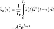
The complex implementation of the correlator is shown in Figure 11.20a, and Figure 11.20b shows an equivalent implementation involving real functions identified as the in‐phase and quadrature components of ![]() . The LPFs provide time averaging over the estimation interval Te as indicated in (11.24). The integration or filtering is fundamental to the correlation processing and is intended to reduce the influence of the additive noise associated with the received signal; the output noise is complicated by the multiplication resulting in products involving S × N and N × N. The correlation lag delay τ is selected to provide the greatest unambiguous range in the frequency estimation as described later.
. The LPFs provide time averaging over the estimation interval Te as indicated in (11.24). The integration or filtering is fundamental to the correlation processing and is intended to reduce the influence of the additive noise associated with the received signal; the output noise is complicated by the multiplication resulting in products involving S × N and N × N. The correlation lag delay τ is selected to provide the greatest unambiguous range in the frequency estimation as described later.

FIGURE 11.20 Phase discriminator implementations.
Referring to (11.24), the angle between the in‐phase and quadrature terms of ![]() is given by15
is given by15

To avoid ambiguities with ± frequency uncertainties it is necessary that the maximum unknown frequency correspond to a correlator output phase <π radians and by solving (11.25) for fε with ϕ = π the condition is
Allowing for some guard range in a noisy environment, it is prudent to require that
where |ϕmax| < π radians. These relationships are depicted by the FD phase diagrams in Figure 11.21 where the frequency error is given by

FIGURE 11.21 Phase‐frequency response of frequency discriminator.
Defining ϕmax in terms of the guard range as a fraction, η of π radians, such that,
then (11.27) is expressed as
Equation (11.28) is the estimate of the frequency error based on the discriminator phase error. Although evaluation of the phase estimate using the inverse tangent function is computationally complex, there are two major advantages: the estimate is linear with frequency and independent of signal amplitude A.
The imaginary part of ![]() can also be used to form the discriminator response expressed as
can also be used to form the discriminator response expressed as

Approximating (11.31) for small arguments and solving for the frequency error results in
This form of the discriminator is similar to that used in the Costas implementation of the PLL; however, unlike (11.25), the response given by (11.31) is not linear over the entire unambiguous frequency range as seen by the two responses shown in Figure 11.22. Furthermore, the unambiguous range of (11.31) is limited to |fτ| < 0.25. The following case study uses the linear atan2 discriminator implementation and examines the frequency estimation error under several signal‐to‐noise conditions.

FIGURE 11.22 Frequency discriminator responses.
The FD can also be used to estimate various derivatives of the signal phase function by cascading additional fixed lag‐delay correlators. For example, the frequency estimate ![]() and frequency‐rate estimate
and frequency‐rate estimate ![]() are implemented as shown in Figure 11.23. In this case, the input phase function is expressed as
are implemented as shown in Figure 11.23. In this case, the input phase function is expressed as


FIGURE 11.23 Frequency and frequency‐rate discriminator.
The details in demonstrating the frequency and frequency rate estimates in Figure 11.23 are left as an exercise (see Problem 9).
11.2.2.5 Case Study: Discriminator Frequency Estimation
The frequency estimation performance and the probability of correctly declaring the frequency using the discriminator shown in Figure 11.20 are examined in this case study. The evaluation is based on the normalized form of the key equation (11.26) obtained by dividing by the Nyquist band frequency ![]() yielding
yielding

Two practical observations are made concerning (11.34). First, to provide a frequency guard range against an unambiguous frequency estimate with additive noise, the normalized form of (11.30) is
The second observation is based on the sampled data processing requiring that the discriminator delay be integrally related to the sampling frequency, that is, τ = n/fs where n is an integer. Recognizing that fs = 2fN, the denominator of the right‐hand side of (11.34) and (11.35) is simply fsτ and the maximum normalized frequency range satisfying the integer requirement occurs when fsτ = 1, that is, when the discriminator delay is one sample, and (11.35) becomes
The phase and frequency estimates are computed at the output of the LPFs shown in Figure 11.20 and the accuracy of these estimates with signal and noise is a function of the signal‐to‐noise ratio and the estimation interval Te = 1/fB where fB is the bandwidth of the LPFs as discussed in Section 1.9.2.1.
As an example of this analysis, consider a CW carrier sampled at fs = 19.2 kHz with fN = 9.6 kHz and a guard interval of η = 0.3 (30%). Based on a simulation of the signal processing in Figure 11.20, with a CW signal source and AWGN channel, the frequency estimation performance of the discriminator is shown in Figures 11.24 and 11.25 as a function for the signal‐to‐noise ratio measured in a sampling frequency bandwidth of 19.2 kHz. The ordinates are plotted in terms of the normalized frequency estimation performance and the example case using the 19.2 kHz sampling frequency. The performance in Figure 11.24 corresponds to a LPF16 bandwidth of fB = 38 Hz with ![]() samples, whereas the performance in Figure 11.25 corresponds to fB = 218 Hz and N = 88 samples. This case was selected to correspond to the 88 bit CW preamble length in the FFT case study of Section 11.2.2.2 with a bit rate of 19.2 kbps. In both cases the number of Monte Carlo acquisition trials at each signal‐to‐noise ratio is 10,000 and the maximum and minimum values correspond to the extremes recorded among the trials for each signal‐to‐noise ratio.
samples, whereas the performance in Figure 11.25 corresponds to fB = 218 Hz and N = 88 samples. This case was selected to correspond to the 88 bit CW preamble length in the FFT case study of Section 11.2.2.2 with a bit rate of 19.2 kbps. In both cases the number of Monte Carlo acquisition trials at each signal‐to‐noise ratio is 10,000 and the maximum and minimum values correspond to the extremes recorded among the trials for each signal‐to‐noise ratio.

FIGURE 11.24 Frequency discriminator estimation performance (fB = 38 Hz, N = 505).

FIGURE 11.25 Frequency discriminator estimation performance (fB = 218 Hz, N = 88).
These results correspond to the worst case frequency error because the input signal frequency error corresponds to fεmax = 6720 Hz as expressed in the normalized form by (11.36). The impact of the LPF bandwidth is evident in these two figures, for example, the performance using the lower bandwidth results in significantly improved estimations and there is no evidence that an unambiguous phase estimate occurred. To the contrary, the degraded performance for the 218 Hz bandwidth case, shown in Figure 11.25, clearly shows the result of the phase measurement reaching through the guard range and causing ambiguous estimates for signal‐to‐noise ratios less than 0 dB. The occurrences of a frequency estimate exceeding the unambiguous frequency range of the discriminator are obvious in the simulation program with a fixed frequency error at, for example, a positive value of fεmax. That is, referring to the phase diagram in Figure 11.21, when ϕ = ϕmax a frequency estimate resulting in a phase estimate π + φ is computed by the atan2(y,x) function as the phase −π + φ radians that corresponds to a negative frequency most likely in the range −fN to −fεmax. Therefore, referring to Figure 11.25, the abrupt negative frequency jump at 0 dB results from the positive frequency exceeding fN. For the 218 Hz LPF bandwidth case, the probability of a phase over‐flow, as described earlier, for signal‐to‐noise ratios of −4.0 and −0.5 dB is 1.49e−2 and 1e−4, respectively.
Although, as described earlier, the ambiguous frequency estimate cannot be discerned in the CW segment, signal verification performed during the synchronization preamble segment will most likely fail because the PLL pull‐in frequency is exceeded. However, the initial CW segment ambiguous frequency estimate can also be verified by correcting the frequency and repeating the CW segment estimation processing using a smaller estimation range fε by increasing the value of τ as in (11.27); this verification processing may have to be repeated to account for the sign ambiguity of the initial estimate. When τ is varied in multiples of two the processing is similar to that of a radix‐2 pipeline FFT thus improving the frequency estimation accuracy.
The frequency detection or CW acquisition probability is evaluated by examining the standard deviation of the phase estimates ϕεn computed by the atan2(y,x) function over the estimation interval of N samples as defined earlier. This criterion is chosen because during the CW preamble, the phase standard deviation is zero without noise and because it increases inversely with the signal‐to‐noise ratio. The functional processing for the CW acquisition or signal present detection is shown in Figure 11.26; also shown is the frequency correction of the input signal ![]() that is used in the symbol synchronization preamble segment. The angular frequency estimate is
that is used in the symbol synchronization preamble segment. The angular frequency estimate is ![]() where the index i is available from the system sample clock generator such that t = ti = iΔt = i/fs.
where the index i is available from the system sample clock generator such that t = ti = iΔt = i/fs.

FIGURE 11.26 Frequency discriminator and detection implementation.
The frequency detection analysis evaluates the performance for the case of fB = 218 Hz (N = 88 samples) corresponding to Figure 11.25. Because the processing of the received signal samples by the FD is sequential, in that, the sampled data is continuously passing through the detection algorithm, much like the pipeline FFT, a detection hypotheses is made at regularly spaced intervals using 75% or ![]() of the most recently collected samples; this reduces the possibility of initial transients influencing the detection. With this understanding, the mean and standard deviation are computed over the most recent N′ = 66 phase samples ϕεn as expressed by (11.18) and (11.19) by substituting
of the most recently collected samples; this reduces the possibility of initial transients influencing the detection. With this understanding, the mean and standard deviation are computed over the most recent N′ = 66 phase samples ϕεn as expressed by (11.18) and (11.19) by substituting ![]() and using the unprimed summations, that is, no censoring of the N′ samples is used. Letting
and using the unprimed summations, that is, no censoring of the N′ samples is used. Letting ![]() and using the normalizing frequency fnorm = 200 Hz the threshold, Thr, is selected to meet the detection and false‐alarm requirements defined as
and using the normalizing frequency fnorm = 200 Hz the threshold, Thr, is selected to meet the detection and false‐alarm requirements defined as
and
These probabilities are evaluated using a histogram, with 200 bins spanning ![]() or 2 kHz, that is used as a probability distribution function. For each signal‐to‐noise ratio, the detection probability is based to 10,000 frequency acquisition trials and the false‐alarm probability is based on 100,000 acquisitions trials with noise only. The performance with and without noise uses an ideal AGC; however, the atan2(y,x) function also provides immunity to the level of the received signal. Based on this description, the detection and false‐alarm performance is shown in Figure 11.27 as the solid and dashed curves, respectively, as a function of the threshold.
or 2 kHz, that is used as a probability distribution function. For each signal‐to‐noise ratio, the detection probability is based to 10,000 frequency acquisition trials and the false‐alarm probability is based on 100,000 acquisitions trials with noise only. The performance with and without noise uses an ideal AGC; however, the atan2(y,x) function also provides immunity to the level of the received signal. Based on this description, the detection and false‐alarm performance is shown in Figure 11.27 as the solid and dashed curves, respectively, as a function of the threshold.
FIGURE 11.27 Frequency detection and false‐alarm performance (fB = 38 Hz case).
The frequency detection results are summarized in Table 11.3 for the indicated detection probabilities and the corresponding threshold and false‐alarm probability. The acceptable operating signal‐to‐noise ratio depends on the application and system specifications and these results illustrate the relationship between the detection and false‐alarm probabilities. Typically the detection probability is specified and the false‐alarm probability is chosen as low as possible to meet other system requirements like the message throughput delay and processor loading. Applications involving automatic repeat request (ARQ) and nonreal time message processing may tolerate higher false‐alarm probabilities. The detection performance characterized for the 88‐bit CW segment, corresponding to fB = 38 Hz, results in reasonable detection probabilities for signal‐to‐noise ratios greater than 0 or 3 dB. Recall that these results represent the worst case conditions corresponding to an initial frequency error of ![]() and the performance with uniformly distributed frequency errors will be somewhat better. Furthermore, by decreasing the LPF bandwidth the operating signal‐to‐noise ratios can be extended into the negative region.
and the performance with uniformly distributed frequency errors will be somewhat better. Furthermore, by decreasing the LPF bandwidth the operating signal‐to‐noise ratios can be extended into the negative region.
TABLE 11.3 Summary of Worst‐Case Detection and False‐Alarm Performance (fB = 38 Hz, N = 88)
| Pd | γ = 4 dB | γ = 3 dB | γ = 0 dB | γ = −1 dB | ||||
| Pfa | Thr | Pfa | Thr | Pfa | Thr | Pfa | Thr | |
| 0.999 | 2.0e−3 | 1.92 | 5e−3 | 2.52 | — | — | — | — |
| 0.99 | 4.7e−4 | 1.44 | 1.5e−3 | 1.80 | 4.0e−2 | 0.48 | — | — |
| 0.95 | 1.7e−4 | 1.08 | 4.1e−4 | 1.44 | 1.1e−2 | 3.12 | 3.0e−2 | 4.32 |
The frequency estimation can be improved by passing the frequency corrected input signal through the FD multiple times, each time improving the frequency of the previous estimate. The estimation improvement is accomplished using the same estimation time Te by decreasing the sampling frequency after the initial estimate has been removed, thereby, reducing the signal bandwidth uncertainty as shown in Figure 11.26. In other words, instead of passing the initial frequency‐corrected signal to the synchronization segment as shown, the corrected signal samples are passed through the frequency decimator a second time using ![]() , corresponding to
, corresponding to ![]() and
and ![]() . This requires that the signal samples over the sliding window of Te seconds be stored in memory and that the rate of the signal processor is commensurate with real‐time processing; the sliding window refers to the estimation interval in consideration of the sequential processing. This refinement of the frequency estimate can be repeated until the estimate falls within the PLL bandwidth as given by (11.3). For a given PLL BLT product, the frequency estimation limit is also dependent on the symbol rate of the underlying received signal modulation and the critical signal‐to‐noise ratio as discussed in Section 10.6.11.
. This requires that the signal samples over the sliding window of Te seconds be stored in memory and that the rate of the signal processor is commensurate with real‐time processing; the sliding window refers to the estimation interval in consideration of the sequential processing. This refinement of the frequency estimate can be repeated until the estimate falls within the PLL bandwidth as given by (11.3). For a given PLL BLT product, the frequency estimation limit is also dependent on the symbol rate of the underlying received signal modulation and the critical signal‐to‐noise ratio as discussed in Section 10.6.11.
The frequency estimate resulting from a second pass through the discriminator is shown in Figure 11.28 corresponding to the first pass estimation results shown in Figure 11.25. The parameters for the pass correspond to the example un‐normalized conditions: fεmax = 0.7fN, fB = 218 Hz, and N = 88 samples with fs = 19.2 kHz, fN = 9.6 kHz, and η = 0.3 (30%). Recalling that the first pass was evaluated for a constant, worse case, frequency offset of fε = fεmax = 6,720 Hz with 10,000 Monte Carlo trials for each signal‐to‐noise ratio, so, for each signal‐to‐noise ratio there are 10,000 independent randomly distributed frequency estimates. Each of these frequency estimates is applied to the discriminator on the second pass using k = 2 with ![]() = fs/2,
= fs/2, ![]() /2, and η′ = η resulting in the performance in Figure 11.28. The means and standard deviations corresponding, respectively, to the first and second passes are summarized in Table 11.4. These results demonstrate the improvement in the frequency estimate resulting from the second pass through the FD as discussed earlier.
/2, and η′ = η resulting in the performance in Figure 11.28. The means and standard deviations corresponding, respectively, to the first and second passes are summarized in Table 11.4. These results demonstrate the improvement in the frequency estimate resulting from the second pass through the FD as discussed earlier.

FIGURE 11.28 Second‐pass frequency discriminator estimation performance (fB = 218 Hz, N = 88).
TABLE 11.4 Comparison of First and Second Pass Frequency Discriminator Performance (fB = 218 Hz, N = 88)
| SNR (dB) | Mean (Hz) | Standard Deviation (Hz) | ||
| Pass 1 | Pass 2 | Pass 1 | Pass 2 | |
| 0 | 4.37 | 0.65 | 375 | 135 |
| 2 | 2.54 | 0.17 | 228 | 84 |
| 4 | 1.55 | 0.11 | 141 | 53 |
| 6 | 0.95 | 0.16 | 89 | 33 |
| 8 | 0.59 | 0.12 | 56 | 21 |
| 10 | 0.36 | 0.12 | 35 | 14 |
11.3 SYMBOL SYNCHRONIZATION PREAMBLE SEGMENT
11.3.1 Introduction
When a CW preamble segment is available prior to the symbol synchronization segment [9], the AGC provides for a constant signal level into the ADC and an initial indication of the presence of a received signal. Furthermore, estimates of the coarse frequency, power, and signal‐to‐noise ratio may be established during the CW preamble segment. Although the knowledge of these parameters simplifies the processing and contributes to an overall reduction in the acquisition time, the symbol synchronization and tracking can be established without a CW preamble segment as may be desirable, for example, in applications involving covert communications. Section 11.3.4 examines the acquisition processing without the aid of the CW preamble segment. In these cases, however, the parameter estimation, or integration, times must be increased to provide the estimation accuracies at the expensed of increased signal processing complexity.
For coherent data demodulation, the synchronization preamble segment processing must estimate [10, 11] and correct the fine frequency and symbol timing and provide for carrier phase and symbol tracking prior to entering the SOM segment. To accomplish these functions with the shortest possible preamble, the demodulator often samples and stores the raw preamble data and performs these functions sequentially making the appropriate correction to the stored data. The last pass through the stored data generally involves phaselock and symbol tracking loops requiring that the final frequency and time estimates are within the initial acquisition limits of the loops.17 Another important consideration is the required acquisition times for each of the loops to achieve steady‐state tracking before the SOM preamble segment; this also influences length of the synchronization segment.
When the CW preamble segment is included, as is often the case, the symbol synchronization segment uses a modulated data sequence that is specifically tailored to aid the demodulator in establishing the symbol timing, verifying the signal presence, and further resolving the frequency estimate. These data sequences typically involve repetitions of short binary data sequence. For example, repeated mark‐space or mark‐mark‐space‐space data patterns or pseudo‐random synchronization codes. Upon establishing and applying the required parameter estimates, symbol and frequency tracking are initiated in preparation for the SOM processing. The SOM detection is typically based on the correlation response of a unique and known relatively long pseudo‐random synchronization sequence with suitable correlation sidelobes so as to minimize false detection of the SOM location. Identifying the time occurrence of the maximum SOM correlation response to within a fraction of a symbol is important because the symbol following the SOM sequence is typically the first information or message header symbol that must be detected correctly or with a sufficiently low probability of error.
Binary sequences with good correlation properties [12–16], principally with low correlation sidelobes, play an important role in the waveform acquisition processing. Commonly used synchronization sequences are as follows: the Barker Codes [17–21], also referred to as perfect, magic, and optimum codes; Williard codes [22, 23]; Neuman–Hofman codes [24, 25]; Gold codes [26]; and Kasami sequences [27]. The number of known Barker codes is limited to those listed in Table 11.5.18 Williard codes are listed in Table 11.6 and Neuman–Hofman codes are listed in Table 11.7 for code lengths up to 24. Walsh codes are discussed in Chapter 7 and correspond to the rows of a Hadamard matrix. Gold codes are generated from linear combinations of M‐sequences and Kasami sequences are subsets of Gold codes with improved correlation responses; both are widely used in spread‐spectrum and code division multiple access (CDMA) applications. M‐sequences are introduced in Chapter 8 and discussed with Gold and Kasami codes in the context of spread‐spectrum waveforms in Chapter 13.
TABLE 11.5 Barker Codes and Correlation Sidelobes
| Code Length | Binary Level | Lead‐Ina | Cyclic | ||
| 2 | + − | — | −1/1 | 0/1 | — |
| 3 | + + − | 0/1 | −1/1 | — | −1/3 |
| 4 | + + − + | 1/1 | −1/1 | 0/3 | — |
| 5 | + + + − + | 1/2 | — | 1/4 | — |
| 7 | + + + − − + − | 0/3 | −1/3 | — | −1/6 |
| 11 | + + + − − − + − − + − | 0/5 | −1/5 | — | −1/10 |
| 13 | + + + + + − − + + − + − + | 1/6 | — | 1/12 | — |
aRepeated analog zeros.
TABLE 11.6 Williard Codes and Correlation Sidelobesa
| Code Length | Binary Level | Lead‐Inb | Cyclic | ||
| 2 | + − | — | −1/1 | 0/1 | — |
| 3 | + + − | 0/1 | −1/1 | — | −1/3 |
| 4 | + + − − | 1/1 | −2/1 | 0/2 | −4/1 |
| 5 | + + − + − | 1/1 | −2/1 | 1/2 | −3/2 |
| 7 | + + + − + − − | 0/2 | −2/1 | — | −1/6 |
| 11c | + + + − + + − + − − − | 2/1 | −3/1 | — | −1/10 |
| 13 | + + + + + − − + − + − − − | 3/1 | −3/2 | 1/6 | −3/6 |
aWilliard [22]. Courtesy of International Society of Automation (ISA).
bRepeated analog zeros.
cSame as inverted and shifted 11‐bit Barker code.
TABLE 11.7 Neuman–Hofman Codes and Correlation Sidelobesa
| Code Length | Binary Level | Lead‐Inb | Cyclic | ||
| 7c | − − − + + − + | 0/3 | −1/3 | — | −1/6 |
| 8 | − − − − + + − + | 1/2 | −2/1 | 0/6 | −4/1 |
| 9 | − − + + + + + − + | 2/1 | −2/1 | 1/6 | −3/2 |
| 10 | − − − − + + − + − + | 2/1 | −2/1 | 2/3 | −2/6 |
| 11c | − − − + + + − + + − + | 0/5 | −1/5 | — | −1/10 |
| 12 | − − + + − − − − − + − + | 2/1 | −3/3 | 4/1 | 0/10 |
| 13 | − − − − − − + + − − + − + | 2/2 | −1/2 | 1/12 | — |
| 14 | − − + + − − + + + + + − + − | 2/1 | −2/2 | 2/4 | −2/9 |
| 15 | − − + + + + + − − + + − + − + | 2/1 | −2/3 | 3/2 | −1/12 |
| 16 | − − − − − + + − − + + − + − + + | 2/1 | −2/4 | 0/12 | −4/3 |
| 17 | − − − − + − + + − − + + + − + − + | 1/6 | −4/2 | 1/8 | −3/8 |
| 18 | − − + + − − + + + + + − + − − + − + | 1/5 | −2/4 | 2/5 | −2/12 |
| 19 | − − − + + + − + + + − + + − + + − + − | 2/1 | −2/6 | 3/2 | −1/16 |
| 20 | − − − + − − − + + + + + − − + − + + − + | 1/4 | −2/1 | 0/14 | −4/5 |
| 21 | − − − − − − + − + + + − + − − + + + − − + | 2/2 | −2/2 | 1/12 | −3/8 |
| 22 | − − − + − − − + + + + + − − + + − + + − + − | 1/8 | −3/3 | 2/7 | −6/2 |
| 23 | − − − − − − + − + − + + − − + + − + − − + + + | 2/4 | −5/1 | 3/6 | −5/4 |
| 24 | − − − − − + + + − − + + + − + − + − + + − + + − | 1/5 | −4/2 | 0/17 | −4/6 |
aNeuman and Hofman [24]. Reproduced by permission of the IEEE.
bRepeated analog zeros.
cSame as Barker code.
Polyphase codes are nonbinary codes that typically result in nonconstant amplitude waveforms and significantly lower correlation sidelobes [28]. Polyphase codes [29] are as follows: Frank codes [30, 31]; Huffman codes [32–36]. Frank codes are generated from the coefficients of the discrete Fourier transform and, for a code of length 16 sidelobe levels ≤ −33 dB relative to the peak correlation are achieved; −43 dB with windowing [37]. Huffman codes are nonbinary polyphase codes that provide for the detection of signals in high Doppler frequency environments.
Tables 11.5 and 11.6 list all of the known Barker and Williard codes, Table 11.7 lists a partial list of the Neuman–Hofman codes, and Table 11.9 contains two long codes used as SOM codes to identify the start of the message header information. In each of these tables the columns labeled ![]() and
and ![]() indicate, respectively, the maximum positive and negative correlation sidelobe levels19 and the number following the backslash is the number sidelobes having these maximum values. The correlation lags represent one code bit. The correlation sidelobes correspond to two noise‐free conditions: the first is denoted as the lead‐in correlation response that results when the received signal is zero preceding the received code; the second condition corresponds to the cyclic correlation response that occurs when the correlation interval always involves elements of the input code. For example, the cyclic correlation response is encountered following the correlation of the first of several contiguously repeated codes. Synchronization preambles containing contiguously repeated codes are discussed in Section 11.3.4.
indicate, respectively, the maximum positive and negative correlation sidelobe levels19 and the number following the backslash is the number sidelobes having these maximum values. The correlation lags represent one code bit. The correlation sidelobes correspond to two noise‐free conditions: the first is denoted as the lead‐in correlation response that results when the received signal is zero preceding the received code; the second condition corresponds to the cyclic correlation response that occurs when the correlation interval always involves elements of the input code. For example, the cyclic correlation response is encountered following the correlation of the first of several contiguously repeated codes. Synchronization preambles containing contiguously repeated codes are discussed in Section 11.3.4.
In many applications the acquisition waveform is specified and it is up to the modem designer to implement the acquisition processing to meet a specified correct acquisition probability (Pca) that consists of several successful events as discussed in Section 11.1. However, the correct acquisition probability is also impacted by the correct message delivery (Pcmd) specification. For example, for a correct message detection probability of Pcm, it is required that ![]() with a specified level of confidence, for example, Pcmd = 0.999 with a confidence level of 95%, at a specified receiver sensitivity. Typically, the correct message detection is based on the data covered by a cyclic redundancy check code as discussed in Section 8.7.
with a specified level of confidence, for example, Pcmd = 0.999 with a confidence level of 95%, at a specified receiver sensitivity. Typically, the correct message detection is based on the data covered by a cyclic redundancy check code as discussed in Section 8.7.
Implementation techniques and performance specifications are available for many commercial systems. For example, the global system for mobile communications is broadly discussed in Mouly and Pautet [7] with references to specifications20 that provide detailed performance and design requirements. The radio interface is the subject of Mouly and Pautet’s Chapter 4 that includes acquisition and synchronization, the channel model, source and channel coding, encryption, burst formatting, and the waveform modulation. Another example of commercial communication systems implementation and performance specification is the CDMA2000 system for mobile and personal communications.21 The preamble acquisition segment waveforms listed in Table 11.8 are example applications for the indicated modulations and symbol rates and two SOM codes are listed in Table 11.9. SOM codes can also be generated by concatenating shorter fixed length codes with appropriate cyclic shifts of the successive fixed length codes that result in desirable or minimum correlation sidelobes. These waveforms illustrate the complexity of the preamble message structure required prior to the detection of the message information.
TABLE 11.8 Example of User Data Preamblesa
| Modulation | Symbol Rate (ksps) | Ch (I/Q) | Preamble Segment | |||||
| CW | Sync | SOM | ||||||
| Bits | Pattern | Bits | Pattern | Bits | Patternb | |||
| BPSK | 9.6 | I | 10 | 0’s | 114 | 110110 | 74 | LPN |
| BPSK | 19.2 | I | 22 | 0’s | 156 | 110110 | 74 | LPN |
| QPSK | 16.0 | I | 14 | 1’s | 111 | 001001 | 37 | LPN |
| Q | 14 | 0’s | 111 | 110110 | 37 | ILPN | ||
| S‐OQPSK | 3.0 and 3.84 | I | 13 | 1’s | 70 | 101010 | 37 | LPN |
| Q | 13 | 0’s | 70 | 111111 | 37 | ILPN | ||
aDefense Information Systems Agency (DISA) [8]. Courtesy of U.S.A. Department of Defense (DOD).
bLPN is Legendre polynomial, ILPN is inverted Legendre polynomial.
TABLE 11.9 SOM LPN Code Bits with Cyclic Correlation Sidelobesa
| Code Length | Code Bits | Lead‐Inb | Cyclic | ||
| 37c | 1110001000010001111010011011101100101 | 4/1 | −3/3 | 1/18 | −3/18 |
| 74 | 1000111010000100111100100001011100011 | 6/2 | −7/1 | 6/8 | −6/18 |
| 0100010011010111101111010110010001011 | |||||
aDefense Information Systems Agency (DISA) [38]. Courtesy of U.S.A. Department of Defense (DOD).
bRepeated analog zeros.
cThe last bit, shown in bold type, is not inverted in the 37‐bit ILPN pattern.
The following figures show the lead‐in and cyclic normalized correlation response of selected codes. The noise‐free correlation responses of the two Barker codes shown in Figure 11.29 demonstrate the lead‐in characteristics when attempting to synchronize to a message preceded by at least two Barker codes. For example, by specifying a normalized detection threshold, the low‐level lead‐in and cyclic correlation sidelobes result in the best synchronization code detection probability among codes of corresponding length. Since the correlation loss with frequency error is a function of the code length, it is typically necessary that a fine‐frequency estimate be performed prior to the code correlation. For very low signal‐to‐noise ratio conditions, as might exist with low‐rate FEC coding, it is necessary to combine several contiguously repeated code correlations to increase the signal‐to‐noise ratio using coherent and/or noncoherent code combining.22 The lead‐in and cyclic correlation sidelobe responses of the Barker codes result in low false‐detection performance leading to their widespread use for message synchronization. Unfortunately longer Barker sequences do not exist; however, the shorter codes are more tolerant to channel dynamics.

FIGURE 11.29 Barker code correlation responses (selected from Table 11.5).
The noise‐free correlation response of four Neuman–Hofman synchronization codes is shown in Figure 11.30 and the lead‐in and cyclic correlation sidelobes are contrasted with those of the Barker codes. Unfortunately, however, the only known Barker codes are listed is Table 11.5 so the Neuman–Hofman codes offer a wider selection of code lengths. For example, the 13‐bit Neuman–Hofman code has two positive correlation sidelobes with levels that are 8.1 dB below the correlation peak compared to 11 dB for the 13‐bit Barker. In contrast, the 24‐bit Neuman–Hofman code has a coherent detection advantage with 13.8 dB lead‐in correlation sidelobes.

FIGURE 11.30 Neuman–Hofman code correlation responses (selected from Table 11.7).
The noise‐free correlation responses of the LPN SOM detection codes listed in Table 11.9 are shown in Figure 11.31. The SOM codes are used to locate the first information symbol and, because the SOM codes are not repeated, only the lead‐in correlation response needs to be considered. However, coherent correlation can be performed because carrier phase and symbol timing tracking have been established during the symbol synchronization processing. In this case, the lead‐in correlations for the length 37 and 74 LPN codes have respective correlation sidelobes of 9.7 and 10.9 dB. However, as indicated in Table 11.8, with BPSK modulation the 74‐bit LPN SOM code is preceded by the repeated 110… data pattern that will alter the lead‐in correlation sidelobes; this is discussed in more detail in Section 11.4. Furthermore, with QPSK‐ and S‐OQPSK‐modulated waveforms, the 37‐bit LPN code is used on the in‐phase rail with the ILPN code on the quadrature rail. With coherent detection, the lead‐in correlation response is improved over the 9.7 dB of the isolated 37‐bit LPN.

FIGURE 11.31 LPN code correlation response.
Although a theoretical correct‐detection probability of the synchronization and SOM codes with additive and multiplicative noise (fading) can be analyzed, it is often beneficial to evaluate the performance using a Monte Carlo simulation program in view of the carrier and symbol tracking and the lead‐in correlation peaks. However, as is always the case, an accurate theoretical analysis will provide a baseline performance measure for the simulated results. In the following subsections, various details of the symbol synchronization preamble are examined.
11.3.2 Frequency and Symbol Time Estimation
Fine‐frequency estimation is performed following the coarse‐frequency estimation obtained from a CW preamble segment. In this case, the frequency search range is significantly reduced and the signal processing focuses on the frequency resolution as opposed to the frequency range.23 In Sections 11.3.2.1 and 11.3.2.2, the description of the symbol time and frequency estimation is based on the mark‐mark‐space‐space preamble data pattern that is known by the demodulator and repeated over the entire synchronization preamble segment. Section 11.3.2.1 describes the joint symbol time and frequency estimation using a FD with knowledge of the symbol rate. The descriptions in Section 11.3.2.2 first resolves and corrects the fine‐frequency estimate over the stored preamble samples and then process the frequency corrected store samples to determine the symbol timing. In this case, the frequency estimation is performed in the frequency domain and, because the symbol rate can also be estimated from the preamble spectrum, it is not necessary to know the symbol rate in advance.
11.3.2.1 Joint Frequency and Symbol Time Estimation Using Discriminator
The approach described in this section to estimate the frequency and symbol or bit timing is based on the FD discussed in Sections 11.2.2.4 and 11.2.2.5. The preamble synchronization segment in this analysis is composed of the 1100 repeated bit pattern and, because the coarse frequency estimate has been removed, the frequency error is a fraction of the bit rate. The detection processing is based on a parallel repetition of the complex discriminator function shown in Figure 11.20a and depicted in Figure 11.32 as a lag‐correlator24 (LC).

FIGURE 11.32 Lag correlator.
The concept involves computing LC outputs for K − 1 hypotheses of the optimum bit timing of the sampled 1100 repeated bit pattern as shown in Figure 11.33. The Ns samples per bit, corresponding to each timing hypothesis, are then used to compute K − 1 lag‐correlator outputs as shown in Figure 11.34. The LC output, corresponding to the optimum bit timing delay relative to the receiver time base, is associated with the imaginary part having the highest mean value and lowest standard deviation or simply having the highest ratio ![]() , such that,
, such that,

FIGURE 11.33 Signal sampling and processing for joint frequency and bit time estimation.

FIGURE 11.34 Lag correlator processing for joint frequency and bit time estimation.
Referring to Figure 11.33, the bits are sampled at intervals of Ts with Ns samples per bit. Relative to the local demodulator time base, the bipolar data is denoted as dn = dn+1 = 1 and dn+2 = dn+3 = −1 corresponds to the repeated binary bit pattern bn = (1100). The demodulator time base can be defined to start anywhere over the sampled data pattern without affecting the detection of the optimum timing delay. Processing the samples over the entire data pattern as shown results in a discriminator delay τ = 2T and, from (11.28), the corresponding LC frequency error is (1 − η)/4T Hz. In this case, the LC spans 4T seconds and the sign of the samples corresponding to the negative data must be changed. This is easily accomplished from the knowledge of the hypothesized timing. Defining the parameter N as the number of sample intervals between each bit time hypothesis, the resulting timing error is
and the number of hypotheses is given by
For example, with Ns = 8 and the requirement Tε = ±T/8 results in N = 2 and K = 16 hypotheses. The timing offsets relative to the demodulator time reference are computed as kNTs where the parameter k represents the k‐th timing hypothesis over the range 0 ≤ k ≤ K − 1.
Referring to Figure 11.34 the inputs into the k‐th LC, denoted as LCk, are computed as

and

The minus sign in (11.43) results from the sign of the data bits dn+2 and dn+3. Using (11.42) and (11.43) in the context of Figure 11.32, the output of LCk is computed as
where ![]() denotes the time average that is implemented as a LPF. Using the bit timing error estimate k′NTs, the local demodulator time base is brought into alignment with the repeated data pattern. The fine‐frequency estimate
denotes the time average that is implemented as a LPF. Using the bit timing error estimate k′NTs, the local demodulator time base is brought into alignment with the repeated data pattern. The fine‐frequency estimate ![]() is determined using the imaginary part of
is determined using the imaginary part of ![]() as described by (11.23) through (11.30). The fine‐frequency estimate is removed from the baseband signal prior to the carrier acquisition and tracking. Following these corrections the bit and frequency acquisition and tracking are executed as described in Section 11.3.5. If the preamble samples have been stored, the acquisition and tracking functions are applied to the time and frequency corrected samples resulting in the most efficient use to the preamble. Reusing the corrected preamble samples results in a shorter preamble and lower message overhead.
as described by (11.23) through (11.30). The fine‐frequency estimate is removed from the baseband signal prior to the carrier acquisition and tracking. Following these corrections the bit and frequency acquisition and tracking are executed as described in Section 11.3.5. If the preamble samples have been stored, the acquisition and tracking functions are applied to the time and frequency corrected samples resulting in the most efficient use to the preamble. Reusing the corrected preamble samples results in a shorter preamble and lower message overhead.
11.3.2.2 Signal Detection and Parameter Estimation Using Signal Spectrum
In this section the coarse‐frequency estimate of the CW preamble segment is refined in the frequency domain for subsequent acquisition and tracking by the PLL. However, as indicated in the introduction, the signal spectrum can also be examined over a wide frequency range with additional signal processing. The focus in this section corresponds to the symbol synchronization segment involving a known data pattern that is used for both fine‐frequency and symbol rate estimation. In this case, the data pattern is uniquely designed to enhance the spectral characteristics for determination of the frequency error and the modulation symbol rate. The spectrum also contains information regarding synchronization to the data pattern; however, the unknown signal phase is problematic in making an unambiguous data pattern synchronization decision. In view of these remarks, the entire preamble is often sampled and stored for processing in the frequency domain and then revisited and processed in the time domain for symbol time synchronization and then revisited a third time for frequency, phase, and symbol tracking. Although, this approach requires more memory and more intense processing to maintain real‐time throughput, the preambles are typically shorter resulting in lower message overhead. Furthermore, in many network applications, the frequency and timing information is stored during network entry allowing for shorter preambles in subsequent transmissions.
The signal parameters involving unique data patterns are examined in the frequency domain relative to the demodulator local time reference as shown in Figure 11.35. Denoting the received symbols in terms of the binary data ![]() suggests that binary PSK modulation is used; however, using the symbol phase notation ϕk,K = kπ/K to denote higher order modulations with a unique data sequence increases the notational complexity that tends to obscure the synchronization concepts. Therefore, the focus in this description is on BPSK modulation.
suggests that binary PSK modulation is used; however, using the symbol phase notation ϕk,K = kπ/K to denote higher order modulations with a unique data sequence increases the notational complexity that tends to obscure the synchronization concepts. Therefore, the focus in this description is on BPSK modulation.

FIGURE 11.35 Received signal timing relative to receiver time‐base.
The analysis that follows uses the analytic baseband description of the received signal expressed as

where τ is the signal delay relative to the demodulator time reference, ωε is the frequency error in radians per second, and φ is a constant phase error. The notation repTo(x) is Woodward’s repetition function [39] with period To = MT, so the data sequence shown in Figure 11.35 is repeated every M symbols as defined in this segment of the preamble. As described in (11.45), the signal phase function is outside of the repTo(x) brackets, so the received signal description corresponds to the phase of the carrier frequency.
Equation (11.45) is a general description of the signal and applies to any repeated data pattern; however, to simplify the analysis, the commonly used preamble synchronization bit pattern of 1100… bits is examined for which M = 4, To = 4T, and d0 = d1 = 1, d2 = d3 = −1 where the unipolar bit to bipolar data translation is di = 2bi − 1. The analysis of the signal spectrum uses the Fourier transform of periodic functions discussed in Section 1.2 for which the spectrum is evaluated as

where fo = 1/To and the Cn are complex coefficients. In the context of (11.45) and the repeated data pattern 1100…, Cn and f(t) are computed as

and
Substituting (11.48) into (11.47) and performing the appropriate integrations, combining of terms, some simplifications, including foT = T/To = 1/4, and then substituting the expression for Cn into (11.46), the spectrum for the repeated data sequence is expressed as

where ![]() . Equation (11.49) is shown in Figure 11.36 for a zero frequency error, that is, fεT = 0. The spectrum is simply shifted to the right or left depending on the frequency error. The discrete spectral lines at f ± 1/4T are of interest and have magnitudes of 2A/π corresponding to a loss of 3.9 dB; the nearest neighbors at f ± 3/4T have magnitudes of 2A/3π resulting in a loss of 13.46 or 9.56 dB below the spectral lines of interest.
. Equation (11.49) is shown in Figure 11.36 for a zero frequency error, that is, fεT = 0. The spectrum is simply shifted to the right or left depending on the frequency error. The discrete spectral lines at f ± 1/4T are of interest and have magnitudes of 2A/π corresponding to a loss of 3.9 dB; the nearest neighbors at f ± 3/4T have magnitudes of 2A/3π resulting in a loss of 13.46 or 9.56 dB below the spectral lines of interest.
FIGURE 11.36 Magnitude of spectral lines of the repeated preamble data pattern 1100 with fε = 0.
The spectral phase function is defined as the phase of F(f) and is expressed as
Upon using λnT, as given earlier, and foT = 1/4, (11.50) is evaluated as

The spectral phase function has a considerable amount of structure, being dependent upon each of the three parameters: τ/T, fεT, and φ. Noting that the bit rate is Rs = 1/T, the frequency tones of interest occur at fu = fε + Rs/4 and fl = fε − Rs/4 corresponding to n = +1 and −1, respectively. For example, these tones rotate linearly in opposite directions by (π/2)τ/T radians, so that over the interval of one data pattern (1100) the phase rotates by 2π radians. These delay‐dependent phase rotations occur independently of the frequency error; however, an additional frequency‐dependent phase of 4πfεT radians is encountered. The unknown signal frequency error fε and phase error φ are problematic in determining the signal delay from the spectral phase information contained in (11.49). However, by determining fu and fl corresponding to the two largest spectral lines, the estimates of the frequency error and bit rate are determined as
and
In many cases, the symbol rate is known and is used to advantage in locating fu and fl when the received signal includes channel and receiver noise. Upon removing the frequency error from (11.51) the signal phase φ remains an impediment to unambiguously determining the signal delay τ/T from the spectral phase function. If, however, the signal phase were successfully removed, the delay estimate can be established to any degree of accuracy with increasing signal‐to‐noise ratio in the measurement bandwidth. For example, for a symbol timing error ![]() , the corresponding accuracy of the spectral phase function is
, the corresponding accuracy of the spectral phase function is ![]() radians. Considering an ℓ‐sigma measurement requirement, the required signal‐to‐noise ratio (γBm) in the measurement bandwidth (Bm) is computed as25
radians. Considering an ℓ‐sigma measurement requirement, the required signal‐to‐noise ratio (γBm) in the measurement bandwidth (Bm) is computed as25

and using ℓ = 3 the required signal‐to‐noise ratio for the 3‐sigma delay estimate is 14.6 dB. In the following case study, the FFT is used to determine the spectrum of the repeated 1100 preamble sequence and the probability of correctly estimating the symbol rate26 and frequency error are examined.
11.3.2.3 Case Study: Detection, Bit Rate, and Frequency Estimation Using BPSK‐Modulated Waveform
In this case study, the FFT is used to determine the spectrum of the repeated 1100 preamble data and the resulting probability of correctly estimating the frequency error is examined when the bit rate is unknown.27 It is assumed that the coarse frequency error of the received signal has been resolved during the CW preamble segment to an accuracy of ![]() . The following description establishes the sampling frequency (fs), the frequency resolution (Δf), the size (Nfft) of the FFT, and the samples per bit (Ns) for the fine‐frequency estimation. Given
. The following description establishes the sampling frequency (fs), the frequency resolution (Δf), the size (Nfft) of the FFT, and the samples per bit (Ns) for the fine‐frequency estimation. Given ![]() and referring to Figure 11.36, the Nyquist band is chosen as BN = 2Rb so the sampling frequency must satisfy the Nyquist condition fs > 2Rb; the value fs = 8Rb is selected.28 The frequency resolution is taken to be one‐fourth of the spectral tone at Rb/4, that is, Δf = Rb/16 from which the size of the FFT is determined as
and referring to Figure 11.36, the Nyquist band is chosen as BN = 2Rb so the sampling frequency must satisfy the Nyquist condition fs > 2Rb; the value fs = 8Rb is selected.28 The frequency resolution is taken to be one‐fourth of the spectral tone at Rb/4, that is, Δf = Rb/16 from which the size of the FFT is determined as ![]() . In the time domain, these parameters result in an estimation interval of
. In the time domain, these parameters result in an estimation interval of ![]() or 16 bits corresponding to four 1100 data pattern repetitions with Ns = 8 samples per bit. If a wider frequency range is desired while maintaining a fixed resolution bandwidth, the sampling rate and antialiasing filter bandwidth can be increased with a commensurate increase in the size of the FFT; in this case, the estimation interval remains the same. On the other hand, if a finer frequency resolution is necessary, the size of the FFT can simply be increased while maintaining the sampling frequency.
or 16 bits corresponding to four 1100 data pattern repetitions with Ns = 8 samples per bit. If a wider frequency range is desired while maintaining a fixed resolution bandwidth, the sampling rate and antialiasing filter bandwidth can be increased with a commensurate increase in the size of the FFT; in this case, the estimation interval remains the same. On the other hand, if a finer frequency resolution is necessary, the size of the FFT can simply be increased while maintaining the sampling frequency.
With a uniformly weight FFT, that is, without windowing, the selection of Δf corresponds to the measurement bandwidth, Bm = Δf, so that a specified received signal‐to‐noise ratio of γb = Eb/No corresponds to a signal‐to‐noise ratio in the measurement bandwidth of

This results in a signal‐to‐noise ratio improvement of 12 dB. However, as indicated in Figure 11.36, the signal‐to‐noise ratio in the FFT cells at fε ± Rb/4 is 3.9 dB lower than given by (11.55) resulting in an improvement of 8.1 dB at each tone frequency of interest. The selection of a smaller Δf will allow a more accurate estimation of the frequency error and bit rate as determined using (11.52) and (11.53).
The simulated spectrums under the foregoing conditions and a normalized frequency error of fεT = 1 are shown in Figure 11.37 for received signal‐to‐noise ratios of Eb/No = 9.6 and 4.1 dB. These signal‐to‐noise ratios correspond, respectively, to uncoded and rate 1/2, K = 7 convolutional coded antipodal modulation performance at Pbe = 10−5. The simulated signal‐to‐noise ratio of each spectral tone, corresponding to n = ±1, is evaluated by establishing the received signal‐to‐noise ratio, given the signal amplitude A, as expressed in (11.45) and then zeroing the signal into the demodulator and computing the total noise power ![]() as the sum of the noise variances on the quadrature rails of the complex spectrum. The resulting simulated signal‐to‐noise ratio, averaged over two independent FFT records, is 17.2 and 12.14 dB for the respective Eb/No values in Figure 11.37. These signal‐to‐noise ratios are simulated in the measurement bandwidth equal to Δf and compare favorably with the theoretical value computed using (11.55) when adjusted by the 8.1 dB loss at the spectral tones at n = ±1. This simple evaluation, or test, goes a long way in confirming the validity simulation.
as the sum of the noise variances on the quadrature rails of the complex spectrum. The resulting simulated signal‐to‐noise ratio, averaged over two independent FFT records, is 17.2 and 12.14 dB for the respective Eb/No values in Figure 11.37. These signal‐to‐noise ratios are simulated in the measurement bandwidth equal to Δf and compare favorably with the theoretical value computed using (11.55) when adjusted by the 8.1 dB loss at the spectral tones at n = ±1. This simple evaluation, or test, goes a long way in confirming the validity simulation.

FIGURE 11.37 Simulated spectrum of repeated 1100 repeated (fεT = 1).
The results of this case study are presented in normalized form, that is, the frequencies are normalized by the bit rate as f/Rb or fT. Because of the frequency normalization and the AWGN channel being considered, the following performance results can be applied to any user bit rate of interest; however, the bit rate must be considered when channels with memory are evaluated. The simulation includes a 145 tap transversal antialiasing filter with a normalized sampling frequency of fsT = 8 and normalized 3 dB cutoff and transition frequencies of fcT = 2 and fTT = 1.5 with a band‐reject attenuation of 50 dB. Figure 11.38 shows the noise‐free spectrums and the antialiasing filter with ![]() and 1.5. The relative magnitudes of the spectral tones at
and 1.5. The relative magnitudes of the spectral tones at ![]() odd integer, when compensated for the 3.9 dB normalizing level used in Figure 11.38, compare favorably with the theoretical values computed using (11.49).
odd integer, when compensated for the 3.9 dB normalizing level used in Figure 11.38, compare favorably with the theoretical values computed using (11.49).

FIGURE 11.38 Simulated spectrum of repeated 1100 repeated (Eb/No = ∞ dB).
The following simulated synchronization performance results are based on 500 Monte Carlo trials for each signal‐to‐noise ratio with the random number generators reinitialized for each signal to noise. For each trail the normalized frequency error is uniformly distributed over the range ![]() . Because the bit rate and frequency error are unknown, the two largest spectral magnitudes found in the bandwidth of the antialiasing filer are used in the estimation process. The frequency estimation for each trial is based on the normalized form of (11.52) where fuT or flT are computed for x = {u,l} as
. Because the bit rate and frequency error are unknown, the two largest spectral magnitudes found in the bandwidth of the antialiasing filer are used in the estimation process. The frequency estimation for each trial is based on the normalized form of (11.52) where fuT or flT are computed for x = {u,l} as
The FFT array has been left shifted by Nfft/2 so that the zero frequency location corresponds to ℓ = Nfft/2 + 1 and the locations ℓl and ℓu are determined from the locations of the two largest spectral magnitudes. Using (11.56) the normalized frequency error estimate, expressed in terms of locations ℓl and ℓu, becomes

Similarly, the bit rate estimate expressed, in terms of locations ℓl and ℓu, is evaluated as
Because the bit rate is unknown, it is essential to estimate the bit rate correctly to establish the two spectral tones for determining the frequency error. The probability that the normalized bit rate is estimated to within 12.5%, that is, ![]() , is shown in Figure 11.39a as a function of the signal‐to‐noise ratio; this resolution corresponds to two frequency resolution cells or 2Δf. Unfortunately, the bit rate estimation is four times more sensitive to errors in the locations ℓl and ℓu than is the frequency estimation (see Problem 13). This is evident from the normalized frequency and bit rate estimation errors shown in Figure 11.39b and c as a function of the signal‐to‐noise ratio.29 The irregularity in the maximum and minimum errors at low signal‐to‐noise ratios occurs because they represent the relatively small sample size of outliers in the 500 samples at each signal‐to‐noise ratio; the random generator seeds are reset for each signal‐to‐noise ratio. The maximum and minimum values for signal‐to‐noise ratio ≥8 dB correspond to a variation of one frequency resolution cell for the frequency and bit rate estimation errors.
, is shown in Figure 11.39a as a function of the signal‐to‐noise ratio; this resolution corresponds to two frequency resolution cells or 2Δf. Unfortunately, the bit rate estimation is four times more sensitive to errors in the locations ℓl and ℓu than is the frequency estimation (see Problem 13). This is evident from the normalized frequency and bit rate estimation errors shown in Figure 11.39b and c as a function of the signal‐to‐noise ratio.29 The irregularity in the maximum and minimum errors at low signal‐to‐noise ratios occurs because they represent the relatively small sample size of outliers in the 500 samples at each signal‐to‐noise ratio; the random generator seeds are reset for each signal‐to‐noise ratio. The maximum and minimum values for signal‐to‐noise ratio ≥8 dB correspond to a variation of one frequency resolution cell for the frequency and bit rate estimation errors.

FIGURE 11.39 Detection and estimation results for repeated 1100 data.
The performance in this case study represents the use of fundamental algorithms and the performance can be improved by using more processing intense techniques. Some examples are as follows:
- Zero padding the FFT will improve the accuracy of the frequency estimation, although the resolution bandwidth remains unchanged.
- Increasing the measurement window, with a commensurate increase in the FFT size. The resolution bandwidth is improved with an accompanying improvement in the measurement signal‐to‐noise ratio.
- Using linear or parabolic interpolation to refine the frequency resolution measurement.
- Using an FFT window to reduce the spectrum leakage into adjacent FFT cells when the signal tones at fT ± n/4 do not fall at the center of an FFT cell.
- Using a higher bit rate estimation tolerance for declaring a successful bit rate acquisition, for example, increasing the 12.5–25%. However, increasing the bit rate estimation tolerance is limited by the acquisition and tracking algorithm requirement discussed in Section 11.3.5.
- Using multiple FFTs and an m‐of‐n decision criterion for declaring a successful bit rate detection.
In many applications the bit rate or a number of possible bit rates are known and the issue becomes one of finding the ℓl and ℓu pairs corresponding to the received bit rate. This can be accomplished by searching through pairs of ℓl and ℓu corresponding to combinations of FFT cells with successively lower magnitudes until the bit rate is found or a limit is reached and a missed bit rate is declared. When the bit rate is declared the frequency estimation is performed using (11.52). The performance improvements listed earlier also apply to the known bit rate case; however, the use of multiple FFTs and the m‐of‐n decision criterion is a major consideration for both detection and confirmation before proceeding to the symbol acquisition and tracking processing.
11.3.2.4 Detection, Symbol Rate, and Frequency Estimation Using MSK‐Modulated Waveform
In this section, the characteristics of the MSK‐modulated waveform spectrum are examined for detection and estimation of the frequency and symbol rate. In this regard, the objectives are identical to those discussed in Section 11.3.2.2; however, the focus is on the unique spectral characteristics of the MSK waveform. The preamble for the multi‐h CPM waveform, discussed in Chapter 9, uses MSK with a symbol rate equal to that of the multi‐h‐modulated user data.
The following descriptions of the MSK‐modulated signal are based on unique data patterns that result in distinct spectral lines at harmonics related to the symbol rate. These spectral characteristics are exploited to estimate the signal presence, carrier frequency, and symbol rates during the synchronization segment of the preamble. The data patterns examined are the repeated sequences 1100… and 10… where the number of repetitions commensurate with the detection and signal‐to‐noise specification based on the system application. For example, the repeated 1100… data is specified for the multi‐h CPM‐modulated waveform preamble and is repeated for a total of 192 bits corresponding to the bit rate of the 2‐h CPM modulation. When mark‐ or space‐hold data is applied to the MSK modulator the transmitted signal is a CW tone corresponding to upper MSK tone fc + Rs/2 and when alternate mark‐space data is applied the lower MSK tone at fc − Rs/2 is transmitted; if required, these tones can serve as a CW preamble. However, when a randomly modulated MSK waveform is squared, the resulting spectrum contains discrete spectral tones, at 2fc ± Rs. These tones can be used for signal detection and synchronization without the necessity of having a CW preamble. The downside of the signal squaring is a decrease in the signal‐to‐noise ratio resulting from the squaring loss and a frequency doubling that requires a higher demodulator sampling frequency. The noise‐free spectrums of the squared MSK‐modulated signal with random and the repeated 1010… data patterns are shown, respectively, in Figure 11.40a and b. The characteristics of the signal processing and the 1024‐point FFT are summarized in Table 11.10. In both of these cases, the spectral lines of interest occur at fc ± Rs.

FIGURE 11.40 MSK acquisition preamble spectrums (1024‐point FFT).
TABLE 11.10 Summary of FFT Processing Parameters
| Nfft | Ns | TfftRs | fres/Rb | η (%) | Gsnr (dB) |
| 1024 | 16 | 64 | 1/32 | 66.7 | 15 |
| 768 | 16 | 48 | 1/24 | 50.0 | 13.8 |
Ns = sample/symbol, TfftRs = Nfft/Ns, fres/Rb = 2/TfftRs, η (%) = 200(Tfft/Rs)/192.
Figure 11.41a shows the noise‐free spectrum of a randomly modulated MSK waveform and is provided as a point of reference for the spectrum of the MSK‐modulated preamble data 11001100… shown in Figure 11.41b; the preamble pattern is repeated for 192 bits. These spectrums are normalized by the maximum level and are based on computer simulations using a 1024‐point FFT as detailed in Table 11.10. The efficiency is a measure of the duration of a single FFT relative to the synchronization preamble length of 192 bits. The 1024‐point FFT occupies 66.7% of the synchronization interval so, to ensure that at least one FFT captures the interval; the FFTs must be overlapped by 33.3%. On the other hand, the 768‐point FFT ensures that at least one FFT captures the interval and, with 50% overlapping, at least two FFTs occupy the synchronization interval. Another important parameter is the signal‐to‐noise ratio improvement, relative to γb = Eb/No, expressed as


FIGURE 11.41 MSK multi‐h CPM acquisition preamble spectrum (1024‐point FFT).
Figure 11.41c and d show the spectrum of the MSK synchronization preamble segment using the 1024‐point FFT for the signal‐to‐noise ratios γb = 6 and 3 dB, respectively. In these cases, the normalized frequency error of the received signal is fεTb = 1. The plots with additive channel noise use different noise seeds so the results are statistically independent. The −23.1 and −29.9 dB spectral lines are buried in the noise; however, spectral lines at fc ± Rs/2 and fc ± Rs exhibit a sufficient signal‐to‐noise ratio, although the variations resulting from the additive noise in the FFT resolution cells are evident.
Figure 11.42a and b are similar to those in Figure 11.41c and d except that the 768‐point FFT is used. The increase in the noise floor is evident; however, there is still a healthy signal‐to‐noise ratio in the cells containing the spectral lines of interest. Referring to Section 9.3.4.1, the minimum γb for the multi‐h CPM modes at Pbe = 10−5 is about 5.3 dB so the synchronization processing for the 3 dB condition using either FFT provides a degree of acquisition robustness. The processing of correctly estimating the frequency error and symbol rate is enhanced by using a weighted sliding window smoothing function across the FFT spectrum cells and selecting the optimum frequency error and symbol rate corresponding to the minimum weighted mean‐square error (MSE) between the sliding window and the magnitudes of the FFT cells. In this case, the weights of the smoothing function are chosen as the magnitude of the three or five symmetrical cells from Figure 11.41b; this approach is similar to the parabolic interpolation discussed in Appendix 2C.

FIGURE 11.42 MSK multi‐h CPM acquisition preamble spectrum (768‐point mixed radix FFT).
11.3.3 Signal Detection and Parameter Estimation Using Correlator
Signal correlation is a convenient technique to determine the symbol time and frequency and, as discussed in the following section, can be used without the CW preamble segment. Correlation processing is used extensively in spread‐spectrum applications to determine code synchronization as discussed in Chapter 13. However, as mentioned previously, the acquisition time and processing complexity is significantly reduced when all of the preamble segments are available.
In the following analysis, the correlator is examined in terms of the baseband BPSK‐modulated received signal ![]() and the demodulator reference signal
and the demodulator reference signal ![]() . The correlation function is expressed as
. The correlation function is expressed as

The delay τ is referred to as the correlation lag and fε and ![]() are the input signal frequency and frequency‐rate errors following the coarse frequency estimation. In practice, the range of the integration in (11.60) is over the duration of the synchronization data pattern denoted as Tp. The synchronization data pattern must have sufficient energy, either signal power or duration, to reliably detect the synchronization code; however, long codes are subject to unacceptable coherent integration losses requiring coherent integration over shorter intervals with noncoherent combining of multiple intervals to achieve the signal to noise required for reliable synchronization. Frequently, a short synchronization code is simply repeated a number of times to achieve the specified synchronization requirements. For example, if the coarse frequency estimate fε is such that the product fεTp results in an unacceptable signal to noise over the correlation interval Tp = NbTb where Nb is the number of code bits of duration Tb, then noncoherent combing of N repeated codes may be performed to achieve the required signal‐to‐noise ratio for synchronization.30
are the input signal frequency and frequency‐rate errors following the coarse frequency estimation. In practice, the range of the integration in (11.60) is over the duration of the synchronization data pattern denoted as Tp. The synchronization data pattern must have sufficient energy, either signal power or duration, to reliably detect the synchronization code; however, long codes are subject to unacceptable coherent integration losses requiring coherent integration over shorter intervals with noncoherent combining of multiple intervals to achieve the signal to noise required for reliable synchronization. Frequently, a short synchronization code is simply repeated a number of times to achieve the specified synchronization requirements. For example, if the coarse frequency estimate fε is such that the product fεTp results in an unacceptable signal to noise over the correlation interval Tp = NbTb where Nb is the number of code bits of duration Tb, then noncoherent combing of N repeated codes may be performed to achieve the required signal‐to‐noise ratio for synchronization.30
Consider the complex received noise‐free baseband BPSK‐modulated signal and the corresponding demodulator reference signal expressed, respectively, as
and
where ![]() represents the received and reference binary data, φ is the unknown constant received signal phase error, and the time‐dependent phase function θε(t) represents the demodulator angular frequency and frequency‐rate errors and is expressed as
represents the received and reference binary data, φ is the unknown constant received signal phase error, and the time‐dependent phase function θε(t) represents the demodulator angular frequency and frequency‐rate errors and is expressed as
In this analysis the demodulator reference signal has unit voltage amplitude. Considering a repeated code length of Nb bits, the correlation response given by (11.60) is evaluated over the code duration Tp as

The notation dn:k refers to the k‐sample misalignment corresponding to the reference delay τ. This expression is best explained by the example depicted in Figure 11.43 using a 7‐bit Barker sequence with Ns = 4 samples per bit. The received baseband sampled signal corresponding to one code interval is sequentially stored in the complex array ![]() and the real sampled local reference is stored in the array sr(iΔT). There are NsNb contiguous stored samples in each array; however, the data samples are not aligned. For example, the stored reference samples are delayed by k = 9 samples from those of the stored received signal samples. The task of the correlator synchronization processing is to determine the optimum correlation lag, τopt, for which dn:k|k=0 = dn for all samples. The resulting code‐bit alignment is used for symbol time and phase tracking in preparation for detecting the SOM location and subsequently the data demodulation. In this example the optimum correlation lag is determined by advancing, or cyclically left shifting, the stored reference bits through
and the real sampled local reference is stored in the array sr(iΔT). There are NsNb contiguous stored samples in each array; however, the data samples are not aligned. For example, the stored reference samples are delayed by k = 9 samples from those of the stored received signal samples. The task of the correlator synchronization processing is to determine the optimum correlation lag, τopt, for which dn:k|k=0 = dn for all samples. The resulting code‐bit alignment is used for symbol time and phase tracking in preparation for detecting the SOM location and subsequently the data demodulation. In this example the optimum correlation lag is determined by advancing, or cyclically left shifting, the stored reference bits through ![]() samples and then associating the optimum lag corresponding to the maximum correlation. As shown in Figure 11.43, the optimum correlation lag correction is seen to be
samples and then associating the optimum lag corresponding to the maximum correlation. As shown in Figure 11.43, the optimum correlation lag correction is seen to be ![]() .
.

FIGURE 11.43 Repeated 7‐bit barker sequences (fεTb = 0, φ = 0, Ns = 4).
In the context of Figure 11.43, consider the transmitted BPSK baseband acquisition waveform with Barker code data ![]() . The simplified31 expression for the transmitted waveform is expressed as
. The simplified31 expression for the transmitted waveform is expressed as
When the transmitted signal is passed through a noiseless channel that introduces a signal phase shift ![]() , the received baseband sampled signal is described as
, the received baseband sampled signal is described as

The simplified BPSK acquisition correlator and demodulator processing is shown in Figure 11.44.
FIGURE 11.44 BPSK acquisition correlator processing.
Using the input described by (11.66), the correlator output samples gc(m) are expressed as
where ![]() is evaluated as
is evaluated as

When m = 0 the ideal correlator output corresponds to the maximum response with ![]() . For the cyclically shifted Barker sequence, the correlation error is ε = −1, for the barker sequences.
. For the cyclically shifted Barker sequence, the correlation error is ε = −1, for the barker sequences.
During the SOM correlation and data detection, the ideal signal phase and timing estimate errors are zero; however, at this stage of the signal acquisition processing the phase is unknown and the effect of the phase‐error terms must be removed using noncoherent detection as shown in Figure 11.44. The sensitivity of the normalized correlator output to a frequency error is evaluated at the zero lag condition when the received and reference signals are perfectly aligned. For BPSK modulation, the correlator sensitivity is evaluated32 as

Substituting the variable x = t/Tp in (11.69) results in the normalized solution

The correlation loss resulting from ![]() are evaluated numerically over the ranges of Tp shown in Figure 11.45 where
are evaluated numerically over the ranges of Tp shown in Figure 11.45 where ![]() . With coherent integration the phase φ is set to zero, however with noncoherent detection this is not necessary. A theoretical solution to (11.69) and (11.70) is provided by Gradshteyn and Ryzhik [40] and, using their results, the magnitude of the correlation function can be shown to be independent of the signal phase. At this point in the acquisition processing, the constant phase error is the least of the concerns, since the PLL will acquire and track the phase prior to the SOM processing. Furthermore, an estimate of the phase can be obtained from the in‐phase and quadrature rails of the peak SOM correlation response to ensure that the PLL does not lock 180 degrees out of phase.
. With coherent integration the phase φ is set to zero, however with noncoherent detection this is not necessary. A theoretical solution to (11.69) and (11.70) is provided by Gradshteyn and Ryzhik [40] and, using their results, the magnitude of the correlation function can be shown to be independent of the signal phase. At this point in the acquisition processing, the constant phase error is the least of the concerns, since the PLL will acquire and track the phase prior to the SOM processing. Furthermore, an estimate of the phase can be obtained from the in‐phase and quadrature rails of the peak SOM correlation response to ensure that the PLL does not lock 180 degrees out of phase.

FIGURE 11.45 Acquisition code correlation loss.
As an example of the correlation processing, the 7‐bit Barker code correlation response is evaluated using a simulation program with ![]() = 0 and Ns = 4 samples per code bit. The simulated coherent detection performance, shown in Figure 11.46a, is ideal sense that fε and φ are also zero. The noncoherent correlation response for a normalized frequency error of fεTp = 0.2 is shown in Figure 11.46b. In this case, the simulated peak correlation response is 0.935 corresponding to a loss of 0.58 dB which is confirmed in Figure 11.45b.
= 0 and Ns = 4 samples per code bit. The simulated coherent detection performance, shown in Figure 11.46a, is ideal sense that fε and φ are also zero. The noncoherent correlation response for a normalized frequency error of fεTp = 0.2 is shown in Figure 11.46b. In this case, the simulated peak correlation response is 0.935 corresponding to a loss of 0.58 dB which is confirmed in Figure 11.45b.

FIGURE 11.46 Repeated 7‐bit barker code correlation response ( = 0, φ = 0, Ns = 4).
The correlator and the CW FFT processing discussed in Section 11.2.2.2 are based on BPSK modulation so, in the following evaluations, the symbol interval corresponds to the bit interval with T = Tb. The overall objective of this section is to reduce the estimates of ![]() to ensure that the phaselock and symbol timing loops are tracking throughout the SOM correlation processing. This is accomplished using noncoherent estimation with an iterative process of adjusting τ to obtain a peak correlation response and then adjusting the frequency and frequency rate to minimize the loss. The normalized frequency error expressed as the product of the frequency error and the observation or estimation interval is defined as
to ensure that the phaselock and symbol timing loops are tracking throughout the SOM correlation processing. This is accomplished using noncoherent estimation with an iterative process of adjusting τ to obtain a peak correlation response and then adjusting the frequency and frequency rate to minimize the loss. The normalized frequency error expressed as the product of the frequency error and the observation or estimation interval is defined as
where fnorm is the normalized CW frequency error that is determined from the specified probability ![]() for a CW signal and the FFT parameters as depicted in Figures 11.15, 11.16, and 11.17. Equation (11.71) gives rise to three system design issues: the accuracy of the CW frequency estimate (fnorm), the duration of the synchronization code (Tp), and the tolerance of the correlator (Loss) given the frequency error. Considering the unweighted, zero‐padded, 256‐point FFT in Figure 11.15 with a sampling rate of fs = 140 kHz, the frequency resolution is computed as fres = 546.875 Hz and the estimation interval is Tp = Tfft = 1.828 ms. Selecting fnorm for
for a CW signal and the FFT parameters as depicted in Figures 11.15, 11.16, and 11.17. Equation (11.71) gives rise to three system design issues: the accuracy of the CW frequency estimate (fnorm), the duration of the synchronization code (Tp), and the tolerance of the correlator (Loss) given the frequency error. Considering the unweighted, zero‐padded, 256‐point FFT in Figure 11.15 with a sampling rate of fs = 140 kHz, the frequency resolution is computed as fres = 546.875 Hz and the estimation interval is Tp = Tfft = 1.828 ms. Selecting fnorm for ![]() = 0.99 corresponding to the best case error estimate with Eb/No = 3 dB results in fnorm = 0.15. Using these parameters and (11.71) results in: fεTp = 0.15, a correlation loss of 0.26 dB, and fε = 82 Hz. The significance of the frequency error depends on the system symbol rate, however, referring to (11.5), for a second order PLL to achieve phase‐lock without cycle skipping requires than fε < FL.
= 0.99 corresponding to the best case error estimate with Eb/No = 3 dB results in fnorm = 0.15. Using these parameters and (11.71) results in: fεTp = 0.15, a correlation loss of 0.26 dB, and fε = 82 Hz. The significance of the frequency error depends on the system symbol rate, however, referring to (11.5), for a second order PLL to achieve phase‐lock without cycle skipping requires than fε < FL.
The length of the synchronization code impacts the correlation gain and the correlation loss as indicated earlier. The signal‐to‐noise ratio at the correlator output is also dependent on the length of the synchronization segment and must satisfy the requirement to declare a correct synchronization probability, Pc(sync). However, the practical length of the synchronization code is dependent on the frequency estimation accuracy and the correlation time of the channel and various system oscillators used for frequency conversion. For example, an off‐the‐shelf, low‐cost, nonovenized oscillator with a correlation time of 0.3 s limits the N‐bit acquisition correlator length to ![]() where Rb is the BPSK‐modulated bit rate. If the resulting correlator output signal‐to‐noise ratio is inadequate to provide the specified synchronization probability then repeated synchronization codes must be included in the synchronization segment and noncoherently combined to achieve the performance results.33 The noncoherent combining of synchronization codes is discussed in the following section.
where Rb is the BPSK‐modulated bit rate. If the resulting correlator output signal‐to‐noise ratio is inadequate to provide the specified synchronization probability then repeated synchronization codes must be included in the synchronization segment and noncoherently combined to achieve the performance results.33 The noncoherent combining of synchronization codes is discussed in the following section.
11.3.4 Synchronization Without CW Preamble Segment
The preamble discussed in this section is based on a known synchronization preamble segment of contiguously repeated N‐bit Barker codes. The focus is on the detection, synchronization, frequency and symbol timing estimation, and PLL tracking without the aid of the CW preamble. The synchronization objective is identical to those discussed previously, namely, to provide for the coherent detection of the SOM sequence. The demodulator synchronization functional processing is shown in Figure 11.47. The following description applies to very low received signal‐to‐noise ratios as might be encountered with turbo coded FEC. This is followed by the more conventional description when operating in high signal‐to‐noise ratio encounters.

FIGURE 11.47 Correlator synchronization and detection processing (signal‐to‐noise ratio: *low, †high).
The signal acquisition and synchronization processing with very low input signal‐to‐noise ratios is described as follows. Using the known range of the received signal frequency uncertainty (|f| ≤ fmax) the demodulator sampling frequency (fs) is established as in (11.7). The ADC Nsc samples spanning the one Barker code interval are mixed to baseband by the coarse reference frequencies (fref,i) and stored as raw data samples over the range of the received signal frequency uncertainty.34 The down‐sampled and low‐pass filtered stored samples result in the equivalent of Ns samples per Barker code bit that are coherently correlated with the stored reference Barker code; cyclic correlation is used to identify the code misalignment. The correlation magnitude is stored in the correlation accumulator forming a (NNs, imax,) time‐frequency noncoherent correlation surface. This provided for a global search over the entire time–frequency uncertainty range. The number of Barker code correlations is determined by the input signal‐to‐noise ratio and the output signal‐to‐noise ratio required to achieve the desired synchronization probability as discussed in Appendix C. Upon completing the noncoherent accumulations a two‐dimensional time–frequency censored CFAR is performed around the largest correlation magnitude. If the CFAR thresholds are pasted a fine‐frequency estimate is established in the same manner around the location of the maximum correlation and phase and symbol time tracking are initiated while searching for the SOM location. If the first CFAR is not passed then the process is repeated for the next four or five largest surface maximums before declaring a missed acquisition.
Examining the entire time–frequency correlation surface prior to performing the CFAF detection processing minimizes the false detections and thereby reduces the average synchronization time when the received signal frequency is uniformly distributed over the entire frequency range. However, if the received signal frequency is, for example, normally distributed about a previously detected mean frequency, the correlation surface search strategy can be improved with a reduction in the average acquisition time. Increasing the length of the synchronization segment by concatenating additional synchronization codes negates the necessity to examine multiple correlation responses over the time–frequency surface; however, the increased preamble duration is unacceptable in many applications. For example, when operating with an input code‐bit signal‐to‐noise ratio of −3.27 dB, choosing the number of synchronization code repetitions so that examining the four highest correlation detections over the time–frequency surface results in a correct synchronization detection of Pc(sync) = 0.99 corresponds to a preamble length that is three to four times shorter than is otherwise required by examining one maximum correlation location.
The signal acquisition and synchronization processing with high input signal‐to‐noise ratios is described as follows. The time–frequency correlations are established using coherent Barker code combining and the CFAR detections are performed sequentially on each frequency hypothesis without the necessity of creating a time–frequency correlation surface. This allows for fewer Barker coded repetitions and much shorter preambles; however, the correlator output signal‐to‐noise ratio must be sufficiently high to result in an acceptable false‐synchronization probability. The fine‐frequency correlation processing is also performed as described earlier to ensure that the frequency estimate is within the lock‐in frequency of the PLL.
The correlation processing shown in Figure 11.47 is based on conventional time‐domain correlation that is performed at each frequency; however, the processor loading is reduced using an FFT correlator [41] in which the spectrum H(m) of the sampled reference and S(m) of the received synchronization code are appropriately stored in the FFT memory. Under these conditions the correlation response is simply obtained as the IFFT of the product S(m)H*(m). Furthermore, the correlation corresponding to a correlation lag of (t − nΔτ) is obtained in the frequency domain correlator through a complex phase shift of ![]() that is efficiently executed in the frequency domain.
that is efficiently executed in the frequency domain.
11.3.5 Symbol and Frequency Acquisition and Tracking
Based on the synchronization preamble segment processing discussed in the preceding sections, the estimate of the carrier frequency error has been adjusted to less than the PLL lock‐in frequency and the symbol timing error is within about 1/8 of the symbol interval or about 1/32 of the symbol interval with RRC modulation. The final task of the synchronization preamble segment is to use these estimates and initialize frequency and symbol acquisition and tracking and ensure that steady‐state tracking occurs prior to the SOM preamble segment. The PLL frequency tracking requirements, functions, and performance are discussed in Chapter 10. The symbol tracking functions are introduced in Sections 2.8.5 through 2.8.7. The E/L gate symbol integrator is used to generate a timing error discriminator response for symbol tracking. In Chapter 4 the symbol timing error generation and tracking functions are shown to be an integral part of the Costas or baseband PLL. Symbol timing adjustments on the order ΔT ≤ T/16 are typical for most modulations; however, for RRC and phase‐shaped modulations adjustments of ΔT ≤ T/64 are recommended.35 The rate of the symbol timing adjust must be controllable with more frequent or larger adjustments during the pull‐in range of the symbol tracking processing. To reduce the impact of the channel and receiver noise on the timing adjustment, the output of the E/L gate discriminator is filtered with a controllable bandwidth that is reduced following the detection of symbol tracking. The symbol rate is typically established by an accurate system clock, whereas received signal carrier frequency is dependent on the dynamics of the channel and the link encounter. Therefore, to minimize the mutual interaction between the two tracking functions, the steady‐state response of the symbol tracking loop should be 8–10 times slower than the carrier tracking loop.
The general implementation of the frequency and symbol tracking functions is shown in Figure 11.48. A major difference in the PLL implementation, from those previously discussed, is that, the known synchronization preamble data, di, is used to aid the carrier frequency acquisition; this is referred to as data‐aided synchronization. Although the preamble data is known from the synchronization processing, it is not known when the synchronization code ends and the SOM code starts, so, the PLL must revert to decision‐directed synchronization using the demodulator data estimates ![]() as soon as possible. This transition is made when the loop lock detector indicates the phaselocked condition.
as soon as possible. This transition is made when the loop lock detector indicates the phaselocked condition.

FIGURE 11.48 Signal phase and timing correction.
The stored samples of the fine‐frequency corrected received baseband signal ŝ(nTs) are used to compute the symbol time error using the E/L gate outputs evaluated as

and

where ![]() ,
, ![]() is the down‐sampled baseband signal corresponding to a symbol error of τ seconds relative to the demodulator reference, and Ns is the number of down‐sampled samples per symbol.36 The E/L output is computed as
is the down‐sampled baseband signal corresponding to a symbol error of τ seconds relative to the demodulator reference, and Ns is the number of down‐sampled samples per symbol.36 The E/L output is computed as

where ![]() is the matched filter output sample. Using the magnitudes to determine the timing error corresponds to noncoherent detection and the performance with additive noise is degraded from that of the coherent detector as expressed in (2.33). Referring to (11.74), when τ > 0 the received signal is delayed relative to the demodulator time base and the output error is positive and when τ < 0 the signal leads the demodulator time base and the error is negative. In either case, the respective samples from the succeeding or preceding symbols corrupt the E/L gate error; however, with selected data patterns, including random data, these contributions are averaged to zero in the E/L filter output resulting in an unbiased estimate.
is the matched filter output sample. Using the magnitudes to determine the timing error corresponds to noncoherent detection and the performance with additive noise is degraded from that of the coherent detector as expressed in (2.33). Referring to (11.74), when τ > 0 the received signal is delayed relative to the demodulator time base and the output error is positive and when τ < 0 the signal leads the demodulator time base and the error is negative. In either case, the respective samples from the succeeding or preceding symbols corrupt the E/L gate error; however, with selected data patterns, including random data, these contributions are averaged to zero in the E/L filter output resulting in an unbiased estimate.
The details of the timing logic in Figure 11.48 are shown in Figure 11.49. The threshold Nthr is dependent upon the timing update increment ΔT and is typically selected during the demodulator simulation and confirmed during hardware testing. After each timing update, the symbol counter is reset to zero to provide hysteresis and avoid over‐correcting of the symbol timing. Following the detection of symbol‐timing lock the threshold is increased to slowdown the timing adjustments during data detection. This can also be accomplished by decreasing the bandwidth of the E/L LPF.37 The symbol‐timing lock detection is not shown in Figure 11.48, however, is obtained by applying the CFAR algorithm to the E/L filter output with lock detection declared in response to a predetermined low timing error variance.

FIGURE 11.49 Timing adjustment logic.
The single‐pole E/L LPF, shown in Figure 11.50, is a recursive filter with the coefficient computed as

FIGURE 11.50 Symbol E/L low‐pass filter.
The normalized bandwidth of the filter is ![]() and the filter gain Ga = 1 − α results in a unit gain response; the gain G and the
and the filter gain Ga = 1 − α results in a unit gain response; the gain G and the ![]() product are available for externally controlled adjustments during system testing.
product are available for externally controlled adjustments during system testing.
11.4 START‐OF‐MESSAGE (SOM) PREAMBLE SEGMENT
The SOM preamble segment is used to locate the first message header bit or the first message information bit if the header is not included in the preamble. This first message bit is identified by the location of the SOM code correlation peak. When the first SOM code bit is encountered, the symbol and frequency tracking loops are locked and operating under their respective steady‐state tracking conditions providing for coherent detection of the SOM bits. Upon initiation of the symbol and frequency acquisition during the synchronization preamble segment, the stored synchronization data bits are shifted through the symbol and phase tracking loops eventually encountering the SOM code bits that lead to the detection of the SOM correlation peak. Although the first bits correspond to those of the synchronization code segment, as the SOM code bits are encountered the SOM lead‐in correlation begins as illustrated by the LPN SOM code correlations in Figure 11.31.38 Throughout the coherent correlation processing a one‐dimensional CFAR detection algorithm is operating looking for a threshold crossing to identify the location of the peak correlation. Since the preamble and message bits are operating at the same symbol rate, the signal‐to‐noise ratio corresponds to the Eb/No required for the message bit detection. Therefore, for a SOM sequence of N bits, the gain in the signal‐to‐noise ratio corresponding to the peak correlation output is 10log10(N) dB. For example, the 74‐bit LPN SOM code detection signal‐to‐noise ratio is 18.7 dB above the operating Eb/No. The detection and false‐alarm probabilities for coherent detection are characterized in Appendix C. Consider, for example, a SOM false‐alarm probability of Pfa ≤ 10−3 is specified and the operating signal‐to‐noise ratio is Eb/No = 6.3 dB. Using the 74‐bit LPN SOM code the SOM detection signal‐to‐noise ratio is γsom = 25 dB and, considering the N − 1 = 73 false‐alarm opportunities, the false alarm per bit must be Pfa(bit) ≤ Pfa/N = 1.37 × 10⁻⁵. Referring to Figures C.2 or C.3 the corresponding correct SOM detection is Pc(SOM) ≥ 0.999 for a signal‐to‐noise ratio ≥14.3 dB so the 25 dB signal‐to‐noise ratio is more than sufficient to achieve a SOM detection probability39 of 0.999.
11.5 SIGNAL‐TO‐NOISE RATIO ESTIMATION
In the concluding sections of this chapter, various methods of estimating the received signal and noise powers and the resulting signal‐to‐noise ratio are discussed. Estimation of these received signal parameters is an important aspect of the signal acquisition processing for determination of the link quality. For example, signal‐to‐noise estimates are often reported to network controllers for the purpose of power control and network configuration management. These estimates are also used in the demodulator for: establishing the optimum PLL operation, diversity combining, as discussed in Chapter 18 and Section 20.9; detection of Reed–Solomon symbol erasures; soft‐decision Viterbi decoding; and detection of extended signal fading or loss‐of‐signal conditions for the purpose of temporally suspending the demodulator tracking functions. System specifications often require that bit count integrity is maintained for a specified time following a signal outage with a specified probability and confidence level of recovering bit synchronization when the signal is recovered. The design challenge is to rapidly detect the signal loss and terminate all tracking functions while maintaining the intrinsic synchronization accuracy based on the parts‐per‐million (ppm) specification of the local oscillators and system clocks.
Although the focus of this section is on the signal‐to‐noise ratio estimation, the estimation of the bit error rate (BER) is also an important demodulator signal quality measure. Newcombe and Pasupathy [42] document their survey results of various BER estimation techniques and Rife and Boorstyn [43] discuss multiple tone parameter estimation using discrete‐time samples. Pauluzzi and Beaulieu [44] have surveyed several techniques for estimating the signal‐to‐noise ratio. Their survey includes the analysis and simulation of the various techniques and a performance comparison using a common MSE performance metric; the techniques are listed in Table 11.11. Based on their study the following conclusions are made: if the data is known at the demodulator, as for example, during acquisition and training intervals, the ML and SNV are superior. With unknown data, the best performing estimators are the ML, SNV, and M2M4, which, coincidently, are the easiest of the techniques to implement.
TABLE 11.11 Signal‐to‐Noise Estimation Techniquesa
| Technique | Remarksb |
| Split‐symbol moments estimator [45–47] (SSME) | Unknown data, Ns ≥ 1 |
| BPSK only with real AWGN | |
| Channel dependent | |
| Processing intense | |
| Maximum‐likelihood estimator [48, 49] (ML) | Unknown and known data, Ns ≥ 1 |
| Real or complexc samples | |
| Estimation bias compensation | |
| Squared signal‐to‐noise variance estimator [50] (SNV) | Unknown or known data, Ns = 1 (MF samples) |
| Real or complexc samples | |
| Estimation bias compensationc | |
| Second‐ and fourth‐order moments estimator [51, 52] (M2M4) | Independent of data, Ns = 1 (MF samples) |
| Realc or complex samples | |
| Unaffected by unknown carrier phase | |
| Signal to variation ratio estimator [53] (SVR) | Unknown data, Ns = 1 (MF samples) |
| Realc or complex samples (MPSK only) | |
| Unaffected by unknown carrier phase |
aThe unknown and independent of data techniques are also referred to as in‐service estimators. MF refers to matched filter.
bReal samples imply BPSK with real AWGN and complex samples imply MPSK, QAM modulations with complex AWGN.
cExtension by authors Pauluzzi and Beaulieu.
All of the estimators are based on ideal distortion less sampled baseband data‐modulated waveforms with AWGN described as
where ![]() and
and ![]() are the signal and noise power scale factors applied, respectively, to the sampled complex signal modulation and noise functions
are the signal and noise power scale factors applied, respectively, to the sampled complex signal modulation and noise functions ![]() and ñk. The in‐phase and quadrature noise samples are iid Gaussian random variables with zero mean and unit variance. Considering real and symmetric modulation functions the matched filter output samples are as follows:
and ñk. The in‐phase and quadrature noise samples are iid Gaussian random variables with zero mean and unit variance. Considering real and symmetric modulation functions the matched filter output samples are as follows:

where Ns is the number of samples per symbol, ![]() is the k‐th sample corresponding to the n − 1 received symbols, and mℓ is the matched filter impulse response.40 Referring to the matched filter development in Section 1.7, the matched filer output signal‐to‐noise ratio for a carrier‐modulated waveform is expressed in terms of the signal energy, EB, and the one‐sided noise power spectral density (No) as
is the k‐th sample corresponding to the n − 1 received symbols, and mℓ is the matched filter impulse response.40 Referring to the matched filter development in Section 1.7, the matched filer output signal‐to‐noise ratio for a carrier‐modulated waveform is expressed in terms of the signal energy, EB, and the one‐sided noise power spectral density (No) as
In general, EB = Ps/B where B is the bandwidth in which the noise power is measured; in the following evaluation of the signal‐to‐noise ratio estimation techniques B = Rb so the signal energy corresponds to the energy per bit, denoted as Eb. The following sections outline the estimation processing of several techniques, as formulated by Pauluzzi and Beaulieu and listed in Table 11.11. The concluding sections provide two case studies of the estimation performance. Estimates of the signal‐to‐noise ratio are often required for network control and, based on Monte Carlo simulations in AWGN channels,41 reasonable expectations of the estimation accuracies are indicated in Table 11.12.
TABLE 11.12 Reasonable signal‐to‐noise estimation accuracies (γ = Eb/No in dB)
| Specified | Accuracy |
| 2.5 ≤ γ ≤ 12 | ±0.5 |
| 12 < γ ≤ 22 | ±1.5 |
| 22 < γ ≤ 32 | ±3.0 |
11.5.1 Maximum‐Likelihood (ML) Estimator
The maximum‐likelihood signal‐to‐noise estimator applies for an arbitrary number of samples per symbol (Ns) so it can be used to estimate the signal‐to‐noise ratio in an arbitrary bandwidth. The estimators of interest for the complex baseband data‐modulated waveform are expressed as


and

The factor ρc in the denominator of (11.81) is included to reduce the estimation bias and, for complex signals, is given by
In these equations K = NsymNs where Nsym is the number of modulation symbols associated with the estimation interval. The notation ![]() corresponds to the k‐th symbol with the i‐th MPSK phase such that
corresponds to the k‐th symbol with the i‐th MPSK phase such that ![]() , where
, where ![]() is the symbol shaping function and
is the symbol shaping function and ![]() : i = 0, …, M − 1 is the symbol phase modulation with log2(M) binary bits per symbol. After PLL and symbol tracking, BPSK modulation can be viewed as involving real signals with
: i = 0, …, M − 1 is the symbol phase modulation with log2(M) binary bits per symbol. After PLL and symbol tracking, BPSK modulation can be viewed as involving real signals with ![]() and (11.79), (11.80), and (11.81) simply accordingly. For real signals the bias reduction factor is
and (11.79), (11.80), and (11.81) simply accordingly. For real signals the bias reduction factor is ![]() .
.
11.5.2 Squared Signal‐to‐Noise Variance (SNV) Estimator
As indicated in Table 11.11, the SNV estimator applies for Ns = 1 so the estimator data samples correspond to the output of the optimally sampled matched filter. This estimation procedure is based on the first absolute moment and the second moment of the sampled data. In this case, the range of the summation is K = Nsym. For the complex signals, the SNV signal‐to‐noise ratio estimate is computed as42

In this case, the estimation bias reduction factor ρc is identical to (11.82) with K = Nsym. The symbol shaping function has been removed by the matched filter so that ![]() . The estimation for real signals is similar to that described earlier for the ML estimator with
. The estimation for real signals is similar to that described earlier for the ML estimator with ![]() and ρr = K/(K − 3).
and ρr = K/(K − 3).
11.5.3 Second‐ and Fourth‐Order Moments (M2M4) Estimator
The M2M4 also applies for Ns = 1 sample per symbol so the estimate samples correspond to the optimally sampled matched filter output. Benedict and Soong [51] refer to this method as the square‐law moments estimator. In general, the noise power estimate is evaluated in terms of the signal power estimate ![]() as
as
Using (11.84), the estimates for the complex MPSK signal power and signal‐to‐noise ratio are evaluated as
and

The estimates for the real BPSK signal power and signal‐to‐noise ratio are evaluated as
and

The moments for both the real and complex signals are computed using the approximate time averages

and

11.5.4 Case Study Using M2M4 Estimator
This case study examines the performance of the M2M4 estimator for the real signal with BPSK modulation as described by (11.84), (11.87), and (11.88). The results are shown in Figure 11.51 using Nsym = 1000 and 100 matched filter symbol (or bit) samples, respectively. At each signal‐to‐noise ratio 100 Monte Carlo trails (or estimates) are evaluated that form the population for establishing the mean, standard deviation, and extreme values indicated in the figures. These results indicate that the signal power estimation results in negligible variation and bias with increasingly high signal‐to‐noise ratios; however, the noise power and signal‐to‐noise ratio estimates, for commonly encountered ranges of signal‐to‐noise ratio, exhibit large variations with increasing bias at lower signal‐to‐noise ratios. Referring to Figure 11.51c it is seen that the mean signal‐to‐noise estimate enters the specification window at Eb/No = 8.5 dB; the standard deviation at 10.5 dB and the extremes at 12 dB.

FIGURE 11.51 Baseband M2M4 estimation errors (Nsym = 1000 bits, Ntrials = 100).
Figure 11.52 represents the performance when the estimation is based on Nsym = 100 symbol samples. The increased variation is a consequence of the shorter estimation interval. The mean signal‐to‐noise ratio estimation still enters the specification at the same signal‐to‐noise ratio of about 8 dB. If the specification were to include an associated confidence level then an acceptable estimate standard deviation could be determined, for example, by applying the central limit theorem and associating the standard deviation with the Gaussian distribution. In a network application, in which communication and control channels use repetitive messages, the demodulator can average the estimates over several frames, thereby, reducing the variation. However, in a nonfading AWGN channel, averaging will not improve the mean value of the estimate. By using the complex product ![]() in the M2M4 estimator the carrier phase and received data are removed, therefore, the estimation is insensitive to the signal phase and cannot be improved upon using known or demodulator detected data.
in the M2M4 estimator the carrier phase and received data are removed, therefore, the estimation is insensitive to the signal phase and cannot be improved upon using known or demodulator detected data.

FIGURE 11.52 Baseband M2M4 estimation errors (Nsym = 100 bits, Ntrials = 100).
The preceding estimated parameter errors are computed based on the accumulated samples at each signal‐to‐noise ratio. The procedure involves determining the mean, standard deviation, and extremes for each parameter and then performing the following normalization with respect to the true parameter value. For example, using the true or known received power, Ps, the estimated mean signal power is computed as

The plus and minus standard deviation and extremes in the power estimates are denoted as ![]() ,
, ![]() , and
, and ![]() . These estimates are then normalized by the true signal power and plotted in decibels as 10log10(normalized estimate). The standard deviation of the estimate is computed based on the samples comprising a subset of the entire population as discussed in Section 1.13.3.
. These estimates are then normalized by the true signal power and plotted in decibels as 10log10(normalized estimate). The standard deviation of the estimate is computed based on the samples comprising a subset of the entire population as discussed in Section 1.13.3.
11.5.5 Case Study: Estimator Performance Using Independent Signal and Noise Power Estimation
In this case study, the noise power estimate is performed serially at the output of a narrowband filter before the signal is present or in parallel with the signal acquisition during discrete frequency searching over the entire frequency uncertainty range as described in Section 11.3.4. In this case, the noise power estimates are performed at several independent frequency bands to ensure that other signal sources do not influence the estimate. The signal‐plus‐noise power estimate is then performed using any of the preamble segments or simply on random data when signal present is declared. During the independent estimations, the receiver and demodulator AGC levels are monitored and the gain changes are compensated in the estimation processing.
Since there is only one parameter to estimate during an estimation interval a second moment M2 estimator is used to estimate the noise and signal‐plus‐noise powers as

and

where ỹk and ẑk are the complex baseband noise and signal‐plus‐noise samples and K = NsymNs is the number of samples used in forming the estimates. As with the M2M4 estimator, the M2 estimator removes the MPSK and QAM data and carrier phase dependence so symbol timing and matched filter sampling is of no consequence. The noise power estimate is simply expressed by (11.92) and the signal power and signal‐to‐noise ratio are computed as
and

where B is the estimation measurement bandwidth and is converted to the user bit rate bandwidth equal to Rb as ![]() .
.
Figures 11.53 and 11.54 show the M2 estimator performance formatted as described for the M2M4 estimator in the previous section. The AGC gain compensation is assumed to be ideal. The sample sizes of 4000 and 2000 correspond to 1000 and 500 bits, respectively, with Ns = 4 samples per bit BPSK modulation. Therefore, except for the 2 : 1 lower ordinate scale factor, Figure 11.53 is comparable to Figure 11.51 insofar as the sample size is concerned.

FIGURE 11.53 Baseband M2 estimation errors (K = 4000 samples, Ntrials = 100).

FIGURE 11.54 Baseband M2 estimation errors (K = 2000 samples, Ntrials = 100).
With the M2 estimator the mean signal power estimate is nearly exact over the entire range of the signal‐to‐noise ratios and the standard deviation and extreme values diminish with increasing signal‐to‐noise ratios. The mean of the noise power estimate is also nearly exact over the entire range of signal‐to‐noise ratios; however, the standard deviation and extreme values are relatively constant and demonstrate the fluctuations associated with the narrowband white noise. The signal‐to‐noise ratio estimate error follows the trends of the signal and inverse noise power estimates. The influence of the estimation interval or sample size is demonstrated in Figure 11.54. The fluctuations in the estimations are decreased by increasing the sample size either directly or by averaging additional independent measurements of the same sample size.
ACRONYMS
- ADC
- Analog‐to‐digital converter
- AGC
- Automatic gain control
- ARQ
- Automatic repeat request
- AWGN
- Additive white Gaussian noise
- BCI
- Bit count integrity
- BER
- Bit error rate
- BPSK
- Binary phase shift keying
- CDMA
- Code division multiple access
- CFAR
- Constant false‐alarm rate
- CRC
- Cyclic redundancy check (code)
- CW
- Continuous wave
- DOD
- Department of Defense
- E/L
- Early–late (gate)
- FD
- Frequency discriminator
- FDMA
- Frequency division multiple access
- FEC
- Forward error correction
- FFT
- Fast Fourier transform
- GSM
- Global system for mobile communications
- ILPN
- Inverted Legendre polynomial
- ISA
- International Society of Automation
- LC
- Lag correlator
- LOS
- Line of sight
- LPF
- Low‐pass filter
- LPN
- Legendre polynomial
- M2M4
- Second‐ and fourth‐order moments estimator
- MAC
- Medium access control (layer)
- MF
- Matched filter
- ML
- Maximum‐likelihood estimator
- MPSK
- Multiphase shift keying
- MSE
- Mean‐square error
- OL
- open loop
- PCL
- pseudo‐closed loop
- PLL
- Phaselock loop
- PN
- Pseudo‐noise
- POL
- pseudo‐open loop
- PPM
- Parts‐per‐million
- QAM
- Quadrature amplitude modulation
- RRC
- Root‐raised‐cosine
- SLM
- Square‐law moments estimator
- SNR
- Signal‐to‐noise ratio
- SNV
- Squared signal‐to‐noise variance estimator
- SOM
- Start‐of‐message
- S‐OQPSK
- phase‐shaped offset quadrature phase shift keying
- SSME
- Split‐symbol moments estimator
- SVR
- Signal‐to‐variation ratio estimator
- TDMA
- Time division multiple access
- VCO
- voltage controlled oscillator
PROBLEMS
- When using the Costas PLL to acquire a noise‐free QPSK‐modulated waveform, express the received baseband power on each quadrature rail and the total baseband power in terms of the peak signal amplitude A and the phase tracking error ϕε. Then, considering that joint AGC power control and carrier phaselock tracking are used, express the peak signal amplitude on each rail in terms of the AGC rms reference voltage Vref under steady‐state AGC conditions and ideal phase tracking, that is, when
 .
. - Consider that the input to the sampled ADC with infinite amplitude resolution is the AWGN random variable x described as N(0,σn). Determine the AGC reference voltage, Vref, which results in zero discriminator output in the steady‐state AGC condition.
Hint: Vref is determined as the median value of y = |x| and is a linear function of σn. - Repeat Problem 2 when x is described as N(m,σn).
- It is often convenient in a simulation program to implement an ideal or theoretical AGC without the signal processing required to implement a particular AGC algorithm using the sampled received signal plus noise. To this end, define the ideal AGC power as Pagc and express the signal power Ps and the noise power Pn in terms of Pagc and the signal‐to‐noise ratio
 .
. - Consider the specified parameters in Table 11.2, using ρ = 2 FFTs for each CW segment instead of 2.5. Evaluate a new set of computed parameters in Table 11.2 using a radix‐2 FFT that will meet the specifications with ρ = 2.
- Referring to Figure 11.15, the simulated frequency estimates (fnorm) and the corresponding probabilities (0.68, 0.9, 0.99) of a correct estimate (Pce) are listed in the following table for the best case 6 dB and worst case 0 dB conditions. The probabilities correspond to the 1σ, 1.65σ, and 2.58σ sigma values of the normally distributed random variable N(0,σ). Show that the simulated error estimates of fnorm also conform to the theoretical error based on the normal distribution N(0,σ).
Simulated Frequency Estimates
| Pce | fnorm | ||
| Best: 6 dB | Worst: 0 dB | ||
| 0.68 | 0.042 | 0.116 | |
| 0.9 | 0.068 | 0.184 | |
| 0.99 | 0.108 | 0.285 | |
- Evaluate and plot the E/L frequency discriminator responses for the Rectangular, Hanning, and Cosine windows with duration Tw seconds using linear and parabolic interpolation under the following conditions:
- The window frequency responses are separated by ±1/Tw Hz with E/L samples corresponding to ±1/2 Tw.
- The window frequency responses are separated by ±1/2Tw Hz with E/L samples corresponding to ±1/4Tw.
Hint: These windows are characterized Section 1.11. - Show that the frequency discriminator guard band is equal to Δf in Equation (11.7).
- Given the input phase function θi(t) expressed in (11.33), show that the estimation of
 and
and  are established as shown in Figure 11.23 and determine the values of the constants k, k0, and k1, in terms of given parameters.
 - Show the detailed steps in deriving the expression for Cn in (11.47).
- In selecting the FFT parameters for examining the spectrum of the repeated 1100 data pattern show the following:
- That commensurate increases in the number of samples/symbol (Ns) and the FFT size (Nfft) results in an increased Nyquist bandwidth BN while maintaining a constant resolution bandwidth with respect to the symbol rate, that is, Δf/Rs = constant.
- Show that a finer frequency resolution with respect to the symbol rate (Δf/Rs) is achieved for a constant sampling frequency (fs) by increasing the measurement window Tm.
- Following the analysis in Section 11.3.2.2 culminating in (11.49), derive the theoretical spectrum for the repeated 110 repeated data pattern specified for the BPSK‐modulated waveforms in Table 11.8. Draw a sketch of the spectrum similar to that shown in Figure 11.37.
- Referring to the case study in Section 11.3.2.3, show that the sensitivity of the normalized symbol rate estimate
 is four times more sensitive to a frequency location error than that of the normalized frequency estimate
  .
.Hint: Evaluate both estimates using  and
and  . where k is the frequency location error.
 - The case study in Section 11.3.2.3 examined the frequency estimation for a known symbol rate and the evaluation was based on the FFT samples taken over exactly four (4) repetitions of the 1100 data pattern. However, when the symbol rate is unknown the FFT will most likely not be taken over an integer number of data patterns. Evaluate the spectrum when the spectrum is based on an additional fractional repetition of the 1100 data pattern. For example, evaluate the spectrum for a measurement interval of
 where
where  .
. - Referring to (11.65), develop the expression of the correlator output for BPSK modulation using
 and the channel phase function ejϕ.
REFERENCES
- 1. U. Mengali, A.N. D’Andrea, Synchronization Techniques for Digital Receivers, Plenum Press, New York, 1977.
- 2. B.E. Blair, Editor, Time and Frequency: Theory and Fundamentals, National Bureau of Standards Monograph, U.S. Department of Commerce, Washington, DC, May 1974.
- 3. R.E. Cashion, W.J. Klepczynski, K. Putkovich, “The Use of Transit for Time Dissemination,” Journal of the Institute of Navigation, Vol. 26, No. 1, pp. 63–69, Spring 1979.
- 4. D.W. Allan, J. Helwig, “Time Deviation and Time Prediction Error for Clock Specifications, Characterization, and Application,” Position Location and Navigation Symposium (PLANS), pp. 22–28, San Diego, CA, November 1978.
- 5. F.S. Nakamoto, M.P. O’Reilly, C.R. Wolfson, “Time and Frequency Synchronization Issues for Tactical, Strategic, and Mobile Forces EHF SATCOM,” Defense Communications Agency, MILSATCOM Systems Office, Contract DCA 100‐79‐C‐008, Fort Meade, MD, 1979.
- 6. F.S. Nakamoto, R.W. Middlestead, C.R. Wolfson, “Impact of Time and Frequency Errors on Processing Satellites with MFSK Modulation,” International Conference on Communications, ICC‐81, Denver, CO, June 14–18, 1981.
- 7. M. Mouly, M.‐B. Pautet, The GSM System for Mobile Communications, Published by the Authors, Palaiseau, France, 1992.
- 8. U.S.A. Department of Defense (DOD) Interface Standard, MIL‐STD‐188‐183A, Interoperability Standard for 25‐kHz TDMA/DAMA Terminal Waveform (Including 5‐ and 25‐kHz Slave Channels), p. 29, Defense Information Systems Agency (DISA), Fort Meade, MD, March 20, 1998.
- 9. F.M. Gardner, W.C. Lindsey, “Special Issue on Synchronization, Part I,” IEEE Transactions on Communications, Vol. COM‐28, No. 8, pp. 1105–1388, August 1980.
- 10. R. Haeb, H. Meyr, “A Systematic Approach to Carrier Recovery and Detection of Digitally Phase Modulated Signals on Fading Channels,” IEEE Transactions on Communications, Vol. 37, No. 7, pp. 748–754, July 1989.
- 11. A. Vanelli‐Coralli, P. Salmi, S. Cioni, G.E. Corazza, A Polydoros, “A Performance Review of PSP for Joint Phase/Frequency and Data Estimation in Future Broadband Satellite Networks,” IEEE International Conference on Telecommunications 2001, Bucharest, Romania, June 4–7, 2001.
- 12. S.W. Golomb, Sequences with Randomness Properties, Martin Company, Baltimore, MD, June 1955.
- 13. S.W. Golomb, Shift Register Sequences, Holden Day, Inc., New York, 1967.
- 14. M.J.E. Golay, “Complementary Series,” IRE Transactions on Information Theory, Vol. IT‐7, p. 82, April 1961.
- 15. D.C. Coll, “A Survey of Finite Codes for Pulse Compression and Synchronization,” Defense Research Telecommunications Establishment, Communication Laboratory, DRTE Report No. 1152, Ottawa, Canada, October 1963.
- 16. R.H. Pettit, “Pulse Sequences with Good Autocorrelation Properties,” The Microwave Journal, Vol. 10, No. 2, pp. 63–67, February, 1967.
- 17. R.H. Barker, “Group Synchronization of Binary Digital Systems,” W. Jackson, Editor, Communication Theory, pp. 273–287, Academic Press, New York, 1953.
- 18. S.W. Golomb, R.A. Scholtz, “Generalized Barker Sequences,” IEEE Transactions on Information Theory, Vol. IT‐11, p. 533, October 1965.
- 19. D.G. Luenberger, “On Barker Codes of Even Length,” IEEE Proceeding, Vol. 51, No. 1, p. 230, January 1963.
- 20. R. Turyn, “On Barker Codes of Even Length,” IEEE Proceeding, Vol. 51, No. 9, p. 1256, September 1963.
- 21. R.S. Berkowitz, Modern Radar, Analysis, Evaluation and System Design, John Wiley & Sons, Inc., New York, 1965.
- 22. M.W. Williard, “Optimum Code Patterns for PCM Synchronization,” Proceedings of the 1962 National Telemetering Conference, NTC62, Washington, DC, May 23–25, 1962.
- 23. M.W. Williard, “Analysis of a System of Mutually Synchronized Oscillators,” IEEE Transactions on Communication Technology, Vol. 18, pp. 467–483, October 1970.
- 24. F. Neuman, L. Hofman, “New Pulse Sequences with Desirable Correlation Properties,” Proceedings of the National Telemetering Conference, NTC71, pp. 272–281, Washington, DC, April 12–15, 1971. NTC71 is issued as a publication of record by the IEEE Transactions on Aerospace and Electronic Systems. Abstracts are published in the IEEE Transactions on Aerospace and Electronic Systems, Vol. AES‐7, No. 3, pp. 565–571, May 1971.
- 25. J.J. Spilker, Jr., Digital Communications by Satellite, Prentice‐Hall, Inc., Englewood Cliffs, NJ, 1977.
- 26. R. Gold, Properties of Linear Binary Encoding Sequences, Robert Gold Associates, Los Angeles, CA, July 1975.
- 27. E.H. Dinan, B. Jabbari, “Spreading Codes for Direct Sequence CDMA and Wideband CDMA Cellular Networks,” IEEE Communications Magazine, pp. 48–54, September 1998.
- 28. M.R. Schroeder, “Synthesis of Low‐Peak‐Factor Signals and Binary Sequences with Low Autocorrelation,” IEEE Transactions on Information Theory, Vol. IT‐16, pp. 85–89, January 1970.
- 29. U. Somaini, M.H. Ackroyd, “Uniform Complex Codes with Low Autocorrelation Sidelobes,” IEEE Transaction on Information Theory, Vol. 20, pp. 689–691, September 1974.
- 30. R.L. Frank, S.A. Zadoff, “Phase Shift Pulse Codes with Good Periodic Correlation Properties,” IEEE Transaction on Information Theory, Vol. IT‐8, pp. 381–382, October 1962.
- 31. R.L. Frank, “Polyphase Codes with Good Nonperiodic Correlation Properties,” IEEE Transaction on Information Theory, Vol. IT‐9, pp. 43–45, January 1963.
- 32. D.A. Huffman, “The Generation of Impulse‐Equivalent Pulse Trains,” IRE Transaction on Information Theory, Vol. IT‐8, No. 5, pp. S10–S16, September 1962.
- 33. D.L. Huffman, “A Modification of Huffman’s Impulse‐Equivalent Pulse Trains to Increase Signal Energy Utilization,” IEEE Transaction on Information Theory, Vol. IT‐20, p. 559, July 1974.
- 34. D.L. Huffman, “Modified Barker Code Approximating Huffman’s Impulse‐Equivalent Sequence,” IEEE Transaction on Aerospace and Electronic Systems, Vol. AES‐11, No. 4, pp. 437–442, July 1975.
- 35. M.H. Ackroyd, “The Design of Huffman Sequences,” IEEE Transaction on Aerospace and Electronic Systems, Vol. AES‐6, No. 6, pp. 790–796, November 1970.
- 36. M.H. Ackroyd, “Synthesis of Efficient Huffman Sequences,” IEEE Transaction on Aerospace and Electronic Systems, Vol. AES‐8, No. 1, pp. 2–8, January 1972.
- 37. B.H. Cantrell, “Sidelobe Reduction in Polyphase Codes,” Naval Research Laboratory, NRL Report 8108, Washington, DC, April 13, 1977.
- 38. U.S.A. Department of Defense (DOD) Interface Standard, MIL‐STD‐188‐183A, Interoperability Standard for 25‐kHz TDMA/DAMA Terminal Waveform (Including 5‐ and 25‐kHz Slave Channels), p. 30, Defense Information Systems Agency (DISA), Fort Meade, MD, March 20, 1998.
- 39. P.M. Woodward, Probability and Information Theory, with Applications to Radar, Pergamon Press Ltd., London, 1953.
- 40. I.S. Gradshtyen, I.M. Ryzhik, Tables of Integrals, Series, and Products, Corrected and Enlarged Edition, p. 147, Integrals 3 and 4, Academic Press, New York, 1980.
- 41. E.O. Brigham, The Fast Fourier Transform and Its Applications, Prentice‐Hall, Inc., Englewood Cliffs, NJ, 1988.
- 42. E.A. Newcombe, S. Pasupathy, “Error Rate Monitoring for Digital Communications,” Proceedings of the IEEE, Vol. 70, pp. 805–828, August 1982.
- 43. D.C. Rife, R.R. Boorstyn, “Multiple Tone Parameter Estimation from Discrete‐Time Observations,” The Bell System Technical Journal, Vol. 55, No. 9, November 1976.
- 44. D.R. Pauluzzi, N.C. Beaulieu, “A Comparison of SNR Estimation Techniques for the AWGN Channel,” IEEE Transactions on Communications, Vol. 48, No. 10, pp. 1681–1691, October 2000.
- 45. M.K. Simon, A. Mileant, “SNR Estimation for the Baseband Assembly,” Jet Propulsion Laboratory, Telecommunications and Data Acquisition Program Report 42–85, Pasadena, CA, May 15, 1986.
- 46. B. Shah, S. Hinedi, “The Split Symbol Moments SNR Estimator in Narrow‐Band Channels,” IEEE Transactions on Aerospace and Electronic Systems, Vol. ASE‐26, pp. 737–747, September 1990.
- 47. B. Shah, J.K. Holmes, “Improving the Split‐Symbol Moments SNR Estimator,” Jet Propulsion Laboratory, Interoffice Memo. 3338‐90‐223, Pasadena, CA, December 19, 1990.
- 48. R.B. Kerr, “On Signal and Noise Level Estimation in a Coherent PCM Channel,” IEEE Transactions on Aerospace and Electronic Systems, Vol. AES‐2, pp. 450–454, July 1966.
- 49. R.M. Gagliardi, C.M. Thomas, “PCM Data Reliability Monitoring through Estimation of Signal‐to‐Noise Ratio,” IEEE Transactions on Communications, Vol. COM‐16, pp. 479–486, June 1968.
- 50. C.E. Gilchriest, “Signal‐to‐Noise Monitoring,” JPL Space Programs Summary, Vol. IV, No. 37–27, pp. 169–184, June 1966.
- 51. T.R. Benedict, T.T. Soong, “The Joint Estimation of Signal and Noise from the Sum Envelope,” IEEE Transaction on Information Theory, Vol. IT‐13, No. 3, pp. 447–454, July 1967.
- 52. R. Matzner, F. Engleberger, “An SNR Estimation Algorithm using Fourth‐Order Moments,” IEEE International Symposium on Information Theory, Trondheim, Norway, June 1994.
- 53. A.L. Brandao, L.B. Lopes, D.C. McLernon, “In‐Service Monitoring of Multipath Delay and Cochannel Interference for Indoor Mobile Communication Systems,” IEEE International Conference on Communications, Vol. 3, pp. 1458–1462, May 1994.