
17
Video Modulation and Transport
Chapter Outline
Video compression is often performed to reduce the data rate, or bandwidth, necessary for transport. Video is sent over satellite, fiber, coax or copper twisted-pair wires. In practice, multiple video signals are often sent over the same medium simultaneously.
17.1 Complex Modulation and Demodulation
Modulation is the process of taking information bits and mapping them to symbols.
This sequence of symbols is filtered to produce a baseband waveform with the desired spectral properties. The baseband waveform or signal is then upconverted to a carrier frequency, which can be transmitted over the air, through coaxial cable, through fiber or some other medium. At some point in this process a DAC converts the signal to analog, which is amplified and transmitted.
One of the most common and simplest modulation methods is known as QPSK (quadrature phase shift keying). With QPSK, every two input bits will map to one of four symbols, as shown below in Figure 17.1. The complex plane is used in order to represent two dimensions.

Figure 17.1 QPSK constellation.
The bitstream of zeros and ones input to the modulator is converted into a stream of symbols. Each symbol is represented as the coordinates of a location in the I-Q plane. In QPSK, there are four possible symbols, arranged as shown. Since there are four symbols, the input data are arranged as groups of two bits, which are mapped to the appropriate symbol. The arrangement of symbols in the I-Q plane is also called the constellation.
Table 17.1 QPSK symbol mapping Constellation size and bit rate

Another common modulation scheme is known as 16-QAM (quadrature amplitude modulation), which has 16 symbols, arranged as shown in Figure 17.2. Again, don’t worry about the name of the modulation. Since we have 16 possible symbols, each symbol will map to four bits. To put it another way, in QPSK each symbol carries two bits of information, while in 16-QAM, each symbol carries four bits of information.

Figure 17.2 16-QAM constellation.
As shown, 16-QAM is the more efficient modulation method. For simplicity, assume symbols are transmitted at a rate of 1 MHz, or 1 MSPS (normally, this is much higher). Then our system, if using the 16-QAM modulation, will be able to send 4 Mbits/second. If instead QPSK is used in this system, it will be able to send only 2 Mbits/second. We could also use 64-QAM which is an even more efficient constellation. Since there are 64 possible symbols, arranged as eight rows of eight symbols each, each symbol carries six bits of information, and supports a data rate of 6 Mbits/second. A few sample constellation types are shown in Table 17.2.
Table 17.2 Constellation size and bit rate

The frequency bandwidth is primarily determined by the symbol rate. A QPSK signal at 1 MSPS will require about the same bandwidth as a 16-QAM signal at 1 MSPS. Notice the 16-QAM modulator is able to send twice the data within this bandwidth, compared to the QPSK modulator. There is a trade-off however: as the number of symbols increases, it becomes more and more difficult for the receiver to detect which symbol was sent. If the receiver needs to choose from 16 possible symbols which could have been transmitted, rather than choose from from four possibilities, it is more likely to make errors.
The level of errors will depend upon the noise and interference present in the signal, the strength of the signal and how many possible symbols the receiver must select from. In non-line-of-sight systems (cellular phones), there are often high levels of reflected and weak signals due to buildings or other objects blocking the transmission path. In this situation, it is often preferable to use a simple constellation, such as QPSK. Even with a weak signal, the receiver can usually make the correct choice of four possible symbols. Line-of-sight systems, such as satellite systems, have directional receive and transmit antennas facing each other. Because of this, the interfering noise level is usually very low, and complex constellations such as 64-QAM or 256-QAM can be used.
Assuming the receiver is able to make the correct choice from among 64 symbols, three times more bits can be encoded into each symbol, resulting in a 3 × higher data rate. Some adaptive communication systems allow the transmitter to dynamically switch between constellation types depending on the quality of the connection between the transmitter and receiver.
17.2 Modulated Signal Bandwidth
We will examine an example of the QPSK constellation, with a transmission rate of 1 MSPS. The baseband signal is two dimensional, so must be represented with two orthogonal components, which are by convention denoted I and Q.
Consider a sequence of five QPSK symbols, at time t = 1, 2, 3, 4 and 5 respectively. The sequence in the two-dimensional complex-constellation plane will appear as a signal trajectory moving from one constellation point to another over time.
The individual I and Q signals are plotted against time in Figure 17.4. This is a two-dimensional signal, with each component plotted separately. The I and Q baseband signals are generated as two separate signals, and later combined together with a carrier frequency to form a single passband signal.
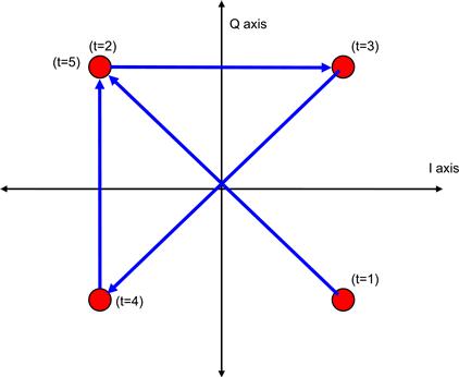
Figure 17.3 Constellation trajectory.

Figure 17.4 Separated component plots.
Note the sharp transitions of the I and Q signals at each symbol. This requires the signal to have high-frequency content. A signal that is of low frequency can change only slowly and smoothly.
The high-frequency content of these plotted I and Q signals can cause problems, because in most systems it is important to minimize the frequency content, or bandwidth, of the signal. We have already discussed frequency response, where a low-pass filter removes fast transitions or changes in a signal (or eliminates the high-frequency components of that signal). If the frequency response of the signal is reduced, this is the same as reducing its bandwidth. The smaller the bandwidth of the signal, the more signal channels and therefore capacity can be packed into a given amount of frequency spectrum. Thus the channel bandwidth is often carefully controlled.
A simple example is FM radio. Each station, or channel, is located 200 kHz from its neighbor. That means that each station has 200 kHz spectrum, or frequency response, it can occupy. The station on 101.5 is transmitting with a center frequency of 101.5 MHz. The channels on either side transmit with center frequencies of 101.3 and 101.7 MHz. Therefore it is important to restrict the bandwidth of each FM station to within + / −100 kHz, to ensures it does not overlap or interfere with neighboring stations. The bandwidth is restricted using a low-pass filter. Video channels are usually several MHz bandwidth, but the same concept applies.
The signal’s frequency response, or spectrum, can be shifted up or down the frequency axis at will, using a complex mixer, or multiplier. This is called up- or downconversion.
17.3 Pulse Shaping Filter
To accomplish frequency limiting of the modulated signal, the I and Q signals are low-pass filtered. This filter is often called a pulse shaping filter, and it determines the bandwidth of the modulated signal. The filter time domain response is also important. Assuming an ideal low-pass filter is used where symbols are generated at a rate (R) of 1 MSPS. The period T is the symbol duration, and equal to 1 in this example. The relationship between the rate R and symbol period T is:
R = 1 / T and T = 1 / R
Alternating with positive and negative I and Q values at each sample interval (this is the worst case in terms of high frequency content), the rate of change will be 500 kHz. So we would start with a low-pass filter with passband of 500 kHz.
This filter will have the sin(x) / x or sinc impulse response. The impulse response is centered in Figure 17-6, along with preceding and following symbol responses. It has zero crossings at intervals of T seconds, and decays slowly. A very long filter is needed to approximate the sinc response. The impulse response of the symbols immediately preceding and following the center symbol are in Figure 17.6 shown below. The signal transmitted will be the sum of all the symbols’ impulse response (we are just showing three symbols here). If the I or Q sample has a negative value for a particular symbol, then the impulse response for that symbol will be inverted from what is shown below.

Figure 17.5 Modulated signal frequency width.

Figure 17.6 Sinc impulse response.
The receiver is sampling the signal at T intervals in time to detect the symbol values. It must sample at the T intervals shown on the time axis above (leave aside for now the question of how the receiver knows exactly where to sample). At time t = −T, the receiver will be sampling the first symbol. Notice how the two later symbols have zero crossings at t = −T, and so have no contribution at this instant. At t = 0, the receiver will be sampling the value of the second symbol. Again, the other symbols, such as first and third adjacent symbols, have zero crossings at t = 0, and have no contribution. If the bandwidth of the filter is reduced to less than 500 kHz (R / 2) then in the frequency domain these pulses would widen (remember that the narrower the frequency spectrum, the longer the time response, and vice versa). Figure 17.7 shows the result if the Fcutoff of the pulse shaping filter is narrowed to 250 kHz, or R / 4.
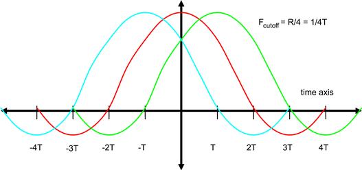
Figure 17.7 Narrow filter impulse response.
In this case, notice how at time t = 0, the receiver will be sampling contributions from all three pulses. At each sampling point of t equal to …−3T, −2T, −T, 0, T, 2T… the signal is going to have contributions from many nearby symbols, preventing detection of any specific symbol. This phenomenon is known as inter-symbol interference (ISI), and shows that transmitting symbols at a rate R requires at least R Hz (or 1 / T Hz) in the passband frequency spectrum. At baseband, the equivalent two-dimensional (complex) spectrum is from −R / 2 to +R / 2 Hz) to avoid creating ISI. Therefore to transmit a 1 MSPS signal over the air, at least 1 MHz of RF frequency spectrum will be required. The baseband filters will need a cutoff frequency of at least 500 kHz.
Notice that the frequency spectrum or bandwidth required depends on the symbol rate, not the bit rate. We can have a much higher bit rate, depending on the constellation type used. For example, each 256-QAM symbol carries eight bits of information, while a QPSK symbol only carries two bits of information. But if they both have a common symbol rate, both constellations require the same bandwidth.
Two issues remain: the sinc impulse response decays very slowly, and so will take a long filter (many multipliers) to implement; and although the response of the other symbols does go to zero at the sampling time when t = N · T, where N is any integer, it can be seen visually that if the receiver samples just a little bit to either side, the adjacent symbols will contribute. This makes the receiver symbol-detection performance very sensitive to the sampling timing.
The ideal would be for an impulse response that still goes to zero at intervals of T, but decay faster and have lower amplitude lobes, or tails. This way, when sampling a bit to one side of the ideal sampling point, the lower amplitude tails will make the unwanted contribution of the neighboring symbols smaller. By making the impulse response decay faster, we can reduce the number of taps and therefore multipliers required to implement the pulse shaping filter.
17.4 Raised Cosine Filter
There is a type of filter commonly used to meet these requirements. It is called the “raised cosine filter”, and it has an adjustable bandwidth, controlled by the “roll off” factor. The trade-off will be that the bandwidth of the signal will become a bit wider, and therefore more frequency spectrum will be required to transmit the signal.
Table 17.3 summarizes the raised cosine response shown in Figure 17.8 for different roll off factors. These labels are also used in Figures 17.9 and 17.10.
Table 17.3 Raised cosine filter frequency rolloff table
| Roll off Factor | Label | Comments – excess bandwidth refers to the percentage of additional bandwidth required compared to ideal low-pass filter |
| 0.10 | A | Requires long impulse response (high multiplier resources), has small frequency excess bandwidth of 10% |
| 0.25 | B | A commonly used roll off factor, excess bandwidth of 25% |
| 0.50 | C | A commonly used roll off factor, excess bandwidth of 50% |
| 1.00 | D | Excess bandwidth of 100%, never used in practice |

Figure 17.8 Raised cosine filter frequency response.

Figure 17.9 Raised cosine impulse response.
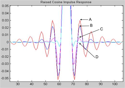
Figure 17.10 Zoomed in raised cosine impulse response.
In Figure 17.8 the frequency response of the raised cosine filter is shown. To better see the passband shape, it is plotted linearly, rather than logarithmically (dB). It has a cutoff frequency of 500 kHz, the same as our ideal low-pass filter. A raised cosine filter response is wider than the ideal low-pass filter, due to the transition band. This excess frequency bandwidth is controlled by a parameter called the “roll off” factor. The frequency response is plotted for several different roll off factors. As the roll off factor gets closer to zero, the transition becomes steeper, and the filter approaches the ideal low-pass filter.
The impulse response of the raised cosine filter is portrayed in Figure 17.9, which shows the filter impulse response, and Figure 17.10 zooms in to better show the lobes of the filter impulse. Again, it is plotted for several different roll off factors. It is similar to the sinc impulse response in that it has zero crossings at time intervals of T (as this is shown in sample domain, rather than time domain, it is not readily apparent from the diagram).
As the excess bandwidth is reduced to approach the ideal low-pass filter frequency response, the lobes in the impulse response become higher, approaching the sinc impulse response. The signal with the smaller amplitude lobes has a larger excess bandwidth, or wider spectrum.
The pulse shaping filter should have a zero response at intervals of T in time so that a given symbol’s pulse response will not have a contribution to the signal at the sampling times of the neighboring symbols. It should also minimize the height of the lobes of the impulse (time) response and have it decay quickly, to reduce the sensitivity to ISI if the receiver doesn’t sample precisely at the correct time for each symbol. As the roll off factor increases, this is exactly what happens in the figures (D). The impulse response goes to zero very quickly, and the lobes of the filter impulse response are very small. However, they have a frequency spectrum that is excessively wide. A better compromise would be a roll off factor somewhere between 0.25 and 0.5 (B and C). Here the impulse response decays relatively quickly with small lobes, requiring a pulse shaping filter with a small number of taps, while still keeping the required bandwidth reasonable.
The roll off factor controls the compromise between:
Another significant aspect of the pulse shaping filter is that it is always an interpolating filter. In the figures, this is shown as a four times interpolation filter. Looking carefully at the impulse response in Figure 17.10, the zero crossing occurs every four samples. This corresponds to t = N · T in the time domain, due to the 4 × interpolation.
The pulse shaping filter must an interpolating filter, as the I and Q baseband signals must meet the Nyquist criterion. In this example, the symbol rate is 1 MSPS. Using a high roll off factor, the baseband spectrum of the I and Q signals can be as high as 1 MHz. So a minimum sampling rate of 2 MHz, or twice the symbol rate, is required. Therefore, the pulse shaping filter will need to interpolate by at least a factor of two, and is often interpolated significantly higher than this.
Using pulse shaped and interpolated I and Q baseband digital signals, digital-to-analog converters create the analog I and Q baseband signals. These signals can be used to drive an analog mixer which can create a passband signal. A passband signal is a baseband signal upconverted or mixed with a carrier frequency. This process can also be done digitally, with a DAC used at much higher frequency to output the signal at the carrier frequency.
For example, using a 0.25 roll off filter for a 1 MSPS modulator, the baseband I and Q signals will have a bandwidth of 625 kHz. Using a carrier frequency of 1 GHz, the transmit signal will require about 1.25 MHz of spectrum centered at 1 GHz.
Until now the transmission path has been our focus. The receive path is quite similar. The signal is down converted, or mixed down to baseband. The demodulation process starts with baseband I and Q signals. The receiver is more complex, as it must deal with several additional issues. There may be nearby signals which can interfere with the demodulation process, which must be filtered out, usually with a combination of analog and digital filters. The final stage of digital filtering is often the same pulse shaping filter used in the transmitter – called a matched filter. The idea is that the same filter that was used to create the signal is also used to filter the spectrum prior to sampling, maximizing the amount of signal energy used in the detection (or sampling process). Because we are using the same filter in the transmitter and the receiver, the raised cosine filter is usually modified to a square-root raised-cosine filter. The frequency response of the raised cosine filter is modified to be the square root of the amplitude across the passband. This also modifies the impulse response as well. This is shown in the figures below, for the same roll off factors.
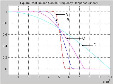
Figure 17.11 Square root raised cosine frequency response.

Figure 17.12 Square root raised cosine impulse response.
Since the signal passes through both filters, the net frequency response is the raised cosine filter. After passing through the receive pulse shaping (also called matched) filter, the signal is sampled. Using the sampled I and Q value, the receiver will choose the constellation point in the I-Q plane closest to the sampled value. The bits corresponding to that symbol are recovered, and if all went well, the receiver has chosen the same symbol point selected by the transmitter. This is very much simplified, but is the essence of a digital communications process.
It can be seen why it will be easier to have errors when transmitting 64-QAM as compared to QPSK. The receiver has 64 closely spaced symbols to select from in the case of 64-QAM, whereas in QPSK there are only four widely spaced symbols to select from. This makes 64-QAM systems much more susceptible to ISI, noise or interference. An option is to just transmit the 64-QAM signal with higher power, to spread the symbols further apart. This is an effective, but very expensive, way to mitigate the noise and interference which prevents correct detection of the symbol at the receiver. Also, the transmit power is often limited by the regulatory agencies, or the transmitter may be battery powered or have other constraints.
The receiver also has a number of other problems to contend with. The sampling is assumed to be at the correct instant in time when one symbol has a non-zero value in the signal. The receiver must determine this correct sampling time, usually by a combination of trial and error during the initial part of the reception, and sometimes by having the transmitter send a predetermined (or training) sequence known by both transmitter and receiver. This process is known as acquisition, where the receiver tries to fine-tune the sampling time, the symbol rate, the exact frequency and phase of the carrier and other parameters which may be needed to demodulate the received signal with a minimum of errors. And once all this information is determined, it must still be tracked, to account for differences in transmit and receive clocks, or other impairments.
Figures 17.13 and 17.14 are plots from both a 16-QAM and 64-QAM constellation after being sampled by an actual digital receiver – a WiMax wireless system operating in the presence of noise. Each receiver signal has the same average energy. The receiver does manage to do a sufficiently good job at detection so that each of the constellation points is clearly visible. As the receiver noise level increases, the constellation samples would quickly start to drift together on the 64-QAM constellation, and it would not be possible to accurately determine which constellation point a given symbol should map to. The 16-QAM system is more robust in the presence of additive noise and other impairments than the 64-QAM.

Figure 17.13 16-QAM recovered constellation.

Figure 17.14 64-QAM recovered constellation.
The modulation and demodulation (modem) ideas presented in this chapter are used in most digital communication systems, including satellite, cable and fiber systems used to transmit video signals. In QPSK all four symbols have the same amplitude. The phase in the complex plane is what distinguishes the different symbols, each of which is located in a different quadrant. For QAM, the amplitude and phase of the symbol is needed to distinguish a particular symbol.
In general, communication systems are full of trade-offs. The most important comes from a famous theorem developed by Claude Shannon which gives the maximum theoretical data bit-rate which can be communicated over a channel, known as the Shannon limit. This depends upon bandwidth, transmit power and receiver noise level, and gives the maximum data rate that can be sent over a channel, or link, with a given noise level and bandwidth.
17.5 Signal Upconversion
The process of mixing a baseband signal onto a carrier frequency is called upconversion, and is performed in the radio transmitter. In the radio receiver, the signal is brought back down to baseband in a process called downconversion. Traditionally, this up- and downconversion process was done using analog signals and analog circuits. Analog upconversion with real (not complex) signals is depicted in Figure 17.15.

Figure 17.15 Analog upconversion.
To see why a mixer works, consider a simple baseband signal of 1 kHz tone and a carrier frequency of 600 kHz. Each can be represented as a sinusoid. A real signal, such as a baseband cosine, has both a positive and negative frequency component. At baseband, these overlay each other, so this is not obvious. But once upconverted, the two components can be readily seen both above and below the carrier frequency.
The equation for the upconversion mixer is:

The result is two tones, of half amplitude, located above and below the carrier frequency.
17.6 Digital Upconversion
Alternately, this process can be done digitally. Let us assume that the information content, whether it is voice, music, or data, is in a sampled digital form. In fact, as we covered in the earlier chapter on modulation, this digital signal is often in a complex constellation form, such as QPSK or QAM, for example.
In order to transmit this information signal, at some point it must be converted to the analog domain. In the past, the conversion from digital to analog occurred when the signal was in baseband form, because the data converters could not handle higher frequencies. As the speeds and capabilities of analog-to-digital converters (ADC) and digital-to-analog converters (DAC) have improved, it has become possible to perform the up- and downconversions digitally, using a digital carrier frequency. The upconverted signal, which has much higher frequency content, can then be converted to analog form using a high-speed DAC.
Upconversion is accomplished by multiplying the complex baseband signal (with I and Q quadrature signals) with a complex exponential of frequency equal to the desired carrier frequency.
The complex carrier sinusoid can be generated using a lookup table, or implemented using any circuit capable of generating two sampled sinusoids offset by 90 degrees. In order to do this digitally, the sample rates of the baseband and carrier sinusoid signal must be equal. Since the carrier signal will usually be of much higher frequency than the baseband signal, the baseband signal will have to be interpolated, or upsampled, to match the sample frequency of the carrier signal. Then the mixing or upconversion process will result in the frequency spectrum shift depicted in Figure 17.16

Figure 17.16 Frequency spectrum of upconversion.
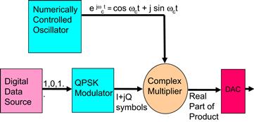
Figure 17.17 Digital upconversion.
For simplicity, assume the output of the modulator is a complex sinusoid of 1 kHz. The equation for this upconversion process is:

This reduces to:
![]()
The imaginary portion is discarded. It is not needed because at carrier frequencies both positive and negative baseband frequency components can be represented by the spectrum above and below the carrier frequency.
The final result at the output of the DAC is:
![]()
Note there is only a signal frequency component above the carrier frequency. This is because the input is a complex sinusoid rotating in the positive (counter clockwise) direction – there is no negative frequency component in this baseband signal.
Normally, as the baseband signal will have both positive and negative frequency components. For example, the complex QPSK modulator trajectory can move both clockwise and counterclockwise depending upon the input data sequence. When upconverted, the positive and negative baseband components will no longer overlay each other, but will be unfolded on either side of the carrier frequency. For example, a baseband signal with a frequency spectrum of 0 to 10 kHz will occupy a total of 20 kHz, with 10 kHz on either side of the carrier frequency. The baseband signal represents the positive and negative frequencies using quadrature form, which is why it is in the form of two dimensional I and Q signals, each with a frequency spectrum from 0 to 10 kHz.
A typical transmit chain in a cable video-distribution system would have many channels digitally modulated and placed upon different carrier frequencies. In this way, many video channels could be carried on the same coax or fiber. The NCO generates the complex exponential signal. This process is shown in Figure 17.18.

Figure 17.18 Digital transmit circuit path.
In this implementation, there are N video channels with 6 MHz bandwidth being sampled at 16 MHz. The next step is to pulse shape and interpolate, or up-sample each video signal by 16, to a sample rate of 256 MHz. Each of these baseband channels is placed upon a different carrier frequency, multiplying by the output of a numerically controlled oscillator (NCO), also running at 256 MHz, which is programmed to the desired carrier frequency.

Figure 17.19 Polyphasing of high rate transmit paths.
The video carriers are all at separate intermediate frequencies, and so can be summed together. At this point, the composite signal can be digitally upconverted to RF frequency. Modern DACs can run at several GHz, and this design uses a DAC running at 4.096 GHz. This can allow for an RF signal in the multi-GHz range out of the DAC, which is filtered and amplified before being transmitted over the cable or broadcast over the air.
Most digital chips cannot clock at 4 GHz. Here, the portions of the circuit with data rates above 256 MHz are built using polyphasing techniques, which involve creating parallel paths in order to process a signal being sampled at rates above the digital clock rate. The sampling rate is stepped up from 256 MHz to 4096 MHz in four stages, each doubling the sample rate, for an overall interpolation of 16.
The actual implementation of this design is shown in Figure 17.20. It is created using a toolflow known as DSPBuilder, from FPGA manufacturer Altera. The toolflow has the capability to automate the polyphasing, or paralleling of high data-rate circuits with a lower FPGA clock rate, in this case, 256 MHz.

Figure 17.20 Implementation in FPGA using Altera’s DSPbuilder toolflow.