
19
Segmentation and Focus
Chapter Outline
The majority of image-processing algorithms require a properly focused image for best results. For some applications this may not be difficult to achieve because the camera capturing the image will have a large depth of field: objects at a wide range of distances from the camera will all appear in focus without having to adjust the focus of the camera. However, for cameras that have narrow depth of field, the image will not always be in focus, and there needs to be some way of assigning a focus score to an image – a measure of focus “goodness”. The focus score serves two purposes:
Out-of-focus images with low focus score can be rejected. This improves the results from image processing algorithms that require focused images and reduces the processing load on these algorithms.
The focus score can be used in the feedback control of a camera autofocus mechanism.
Because focus-score assessment is at the front end of any image-processing system, it has a large impact on system performance. For example, imagine a video stream that contains focused and unfocused images, and feeding these to an image processor that takes one second to process each video frame. The system would be generating a lot of bad results, and also taking a long time to generate a good result. In fact, if the image processor is randomly sampling the incoming video frames (i.e. there is no video storage), it may never produce a good result.
19.1 Measuring Focus
We all recognize focused and unfocused images when we see them. Unfocused images are characterized by blurry and difficult to identify objects, whereas focused images are characterized by well-defined, easily identifiable objects. Let’s take a look at what we mean by objects appearing blurry: an object that appears blurry has edges that are “fuzzy”, and the transition from object to background is gradual. Compare this to a focused image, where the edges of objects are sharp, and the transition from object to background is immediate. The effect of focus on edge sharpness can be seen in Figure 19.1. We can effectively generate a focus score for an image or an object within an image by measuring the sharpness of these edges.

Figure 19.1 Example of focused and unfocused images.
19.1.1 Gradient Techniques
Gradient techniques measure the difference between adjacent pixel grayscale values, and use this as a measure of rate of change of grayscale, or gradient of the gray levels. Focused images exhibit large rates of change in pixel gray level, whereas in an unfocused image the gray level value’s rate of change is lower. Thus we can measure the absolute gradient of every pixel, sum all the gradients and use this as a focus score.
F = ∑y=0 to M − 1 ∑x=0 to N − 1 | i(x + 1,y) − i(x,y) |
Where:
F = Focus score
N = Number of pixels in image row
M = Number of pixels in image column
i(x,y) = Image gray level intensity of pixel (x,y)
| i(x + 1, y) − i(x,y) | > = T
T = Threshold gray level
Let’s calculate the focus score in the horizontal direction for the two images shown in Figure 19.2.

Figure 19.2 Example of focused and unfocused vertical edge.
We’ll set T = 100 and we will firstly calculate the focus score for the unfocused image, with the blurry edge:
F = (250 − 150) × 8 = 800
Note that there is only one difference that is greater than or equal to T. Since every row is the same, we multiply this one diference by the number of rows.
Next we will calculate the focus score for the focused image, with the sharp edge:
F = (250-0) × 8 = 2000
From this calculation we see the focused image has a higher score. Thus for multiple images of the same scene we have a method that can identify images with the best focus.
This rate of change also translates to higher frequencies in the spatial domain, so applying a high-pass filter and then measuring the power of the filtered image gives an indication of the total power of the high-frequency components in the image and thus the focus. Noise within an image can also have high-frequency content: depending on the system, it may be necessary to use a band-pass filter that rejects some of these high frequencies.
19.1.2 Variance Techniques
Since the pixel gray values of edges in a focused image transition rapidly, such images exhibit greater variance in pixel values. We can measure this by calculating the difference between each pixel and the mean value of all the pixels. We square the difference to amplify larger differences, and remove negative values:
F = (1 / MN) ∑y = 0 to M − 1 ∑x = 0 to N − 1 (i(x,y) − μ)2
Where:
μ = Mean of all pixels.
Let’s apply this variance measure to our two images in Figure 19.2. First we we’ll calculate the mean for the unfocused image:
μ = (250 + 250 + 250 + 150 + 100 + 50 + 0 + 0) × 8 / 64 = 131.25
Next we calculate the variance:
F = (1 / 8 × 8) × (((250 − 131.25)2 + (250 − 131.25)2 + (250 − 131.25) 2 + (150 − 131.25)2 +
(100 − 131.25)2 + (50 − 131.25)2 + (0 − 131.25)2 + (0 − 131.25)2) × 8)
Similarly for the focused image:
μ = (250 + 250 + 250 + 250 + 0 + 0 + 0 + 0) × 8 / 64 = 125
F = (1 / 8 × 8) × (((250 − 125)2 + (250 − 125)2 + (250 − 125)2 + (150 − 125)2 + (0 − 125)2 + (0 − 125)2 + (0 − 125)2 + (0 − 125)2) × 8)
F = 15,625
Here we see that the focused image has a higher variance than the unfocused image.
One of the variations on this algorithm divides the final result by the mean pixel value, thus normalizing the result, and compensating for variations in image brightness.
19.2 Segmentation
Until now we have considered the entire image to be in the same level of focus. This may not be the case. For example, images of tiny micro-electro-mechanical-systems (MEMS) may have regions of the image that are in different levels of focus, thus we have to choose the region of the image that we want to be correctly focused. Sometimes this can be as simple as choosing a region in the middle of the image, but it is not always this easy, and there are situations where the region of interest must be located and its focus score calculated. We would need to extract a segment from the image. There are techniques to find the edges in an image, and from this information identify the edges of interest. These techniques are beyond the scope of this chapter – what we will consider here is the simpler case where we know the shape of the region that we want to locate.
19.2.1 Template Matching
The segmentation algorithm uses expanding, shifting shape templates to locate regions within the image. For example, if the target region is a circle, then pixel image data is collected from circular regions of varying radius and position. Summing pixel data in these circular regions gives a gray level score for the region and comparing gray values between circular regions determines the region boundary.
Let’s take a look at the example in Figure 19.3. We are going to locate a square region of 4 × 4 pixels, located within a 12 × 12 image. Since we are looking for a square region, we will use shifting, expanding square templates and match these against the image. Furthermore, since the square region we are trying to locate has uniform gray values, we will only add the values of the pixels on the perimeter of the squares, and ignore the pixel values inside the squares. We will start with a square template of size four at coordinates (6, 6) Figure 19.3(a). First we will add or integrate the values around the square, and normalize by dividing by the total number of pixels:

Figure 19.3 Expanding a square template with × coordinate shift.
S(4) = (12 × 1) / 12 = 1
Where:
S(n) = Sum of all the pixel values around a square with sides of length n.
Similarly for template squares of size 8 and 12:
S(8) = ((11 × 1) + (17 × 0)) / 28 = 0.36
S(12) = (44 × 0) / 44 = 0
Now we calculate the maximum gradient of the integral sums:
G(4,8) = | 1 − 0.36 | = 0.64
G(8,12) = | 0.36 − 0 | = 0.36
Where:
G(n,m) = The gradient between squares of with sides length n, and m.
Thus for expanding squares with origin (6, 6) the maximum gradient is 0.64.
Now we will shift the origin to (5, 6) as shown in Figure 19.3(b). First we calculate the integrals:
S(4) = (12 × 1) / 12 = 1
S(8) = ((6 × 1) + (22 × 0)) / 28 = 0.21
S(12) = (44 × 0) / 44 = 0
And now the gradients:
G(4, 8) = | 1 − 0.21 | = 0.79
G(8,12) = | 0.21 − 0 | = 0.21
Notice that the peak gradient is higher for the second position, where the expanding circles are centered at (5, 6). This tells us that (5, 6) is more likely to be the origin of the square than (6, 6). That is x = 5 is the best candidate for the x coordinate of the origin.
We can perform the same shifting operation in the y direction, and thus find the optimal y coordinate as illustrated in Figure 19.4. If we calculate the gradients we get a similar result to that for the x shifting, and in this case we find that (6, 7) is a better candidate than (6, 6) and thus y = 7 is the best candidate for the y coordinate of the origin. Our best estimate so far for the origin of the target square is x = 5, y = 7 or (5, 7). If we check again we will see that (5, 7) is indeed the origin of the square. In a real example we would not be so lucky, and we would need to repeat the operation a number of times. In each iteration, we would use the newly calculated origin and a reduced step size for the x and y shifts.

Figure 19.4 Expanding square template with y coordinate shift.
We also see that the gradient is larger between the squares of side length four and eight pixels than it is between the squares of side length 8 and 12 pixels. This tells us which template squares are more likely to border the target square. So, in each iteration of the algorithm, as well as reducing the x and y step sizes, we would also use the new best-candidate template-square size, and reduce the step size of the expansion.
In the previous example we used a contour integral to determine the average gray level at each template position. This works well if the region has uniform gray values but, if this is not the case, it may be necessary to perform an area integral instead of a contour integral. This has the effect of averaging the gray values within the template area, and thus reducing the effect of image details.
Once the target region has been located within the image, then one of the focus algorithms previously described can be applied to the region, and a focus score calculated.
Figure 19.5 shows the use of expanding circles to locate the pupil within an image of the eye. The process is similar to the one described for expanding and shifting square templates, but in this case the template is a circle.

Figure 19.5 Expanding circle template applied to image of eye.
19.2.2 FPGA Implementation
Figure 19.6 shows a block diagram of a system designed to perform a contour integral. The base template is stored as x and y coordinates in two separate memories. Template expansion is performed by multiplying the template coordinates by a scaling factor, and the scaled template coordinates are fed to an adder. Here the x and y offset coordinates are added to generate an (x, y) coordinate reference within the image frame. This (x, y) reference must be manipulated to create a linear address within the image frame store. Assuming image rows are stored in contiguous memory blocks, this would involve multiplying y by the image line width and adding x. The generated address can be used to retrieve the pixel data from memory, and the data fed to an accumulator which will sum all the pixel data for the contour defined by the scaled and shifted template.
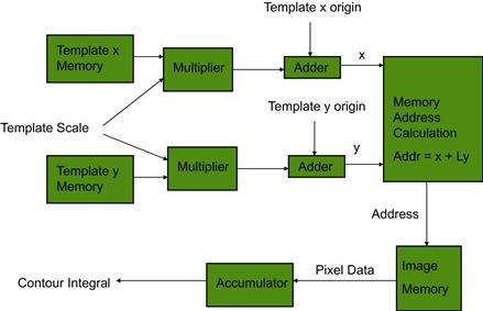
Figure 19.6 Block diagram of a contour integral engine.
By pipelining the operations, it is possible for an FPGA to perform all the operations in parallel, so that memory-access speed becomes the performance limitation. Depending on the image size, it may be possible to store the image in internal FPGA RAM. If this is possible then not only can the memory operate at higher speed, but the dual-port feature of the internal RAM can be used so that two of these contour integral engines can be executed in parallel.