
5
Video Scaling
Chapter Outline
5.1 Understanding Video Scaling
5.2 Implementing Video Scaling
Video comes in different sizes – as anyone who has watched standard definition DVDs on their high resolution HDTVs has no doubt experienced. Each video frame, which consists of lines of pixels, has a different size as shown in Figure 5.1.

Figure 5.1
Video has to be resized to view it on different sized displays – this means that the native resolution of the video frame is adjusted to fit the display available. Video resizing or scaling is an increasingly common function used to convert images of one resolution and aspect ratio to another “target” resolution and/or aspect ratio. The most familiar example of video scaling is scaling a VGA signal (640 × 480) output from a standard laptop to an SXGA signal (1280 × 1024) for display on LCD monitors.
For high-volume systems dealing with standardized image sizes such as HD television, video scaling is most efficiently done using application specific standard products (ASSPs). However, many video applications such as video surveillance, broadcast display and monitoring, video conferencing and specialty displays, need solutions that can handle custom image sizes and differing levels of quality. This often requires custom scaling algorithms. FPGAs with an array of high-performance DSP structures are ideally suited for such algorithms, and FPGA vendors are beginning to offer user-customizable video-scaling IP blocks that can be quickly configured for any application.
Scaling is often combined with other algorithms such as deinterlacing and aspect ratio conversion. In this chapter we will focus on the digital video processing involved in resizing or scaling a video frame.
Towards the end of this chapter we will briefly describe the different aspect ratios since scaling is done many times to stretch a 4:3 image to display on today’s 16:9 HDTV displays.
5.1 Understanding Video Scaling
Video scaling, whether upscaling or downscaling, is the process of generating pixels that did not exist in the original image. To illustrate this, let’s look at a simple example: scaling a 2 × 2 pixel image to a 4 × 4 pixel image, as shown in Figure 5.2. In the “New Image” the white pixels are pixels from the “Existing Image” and the black pixels are those that need to be generated from the existing pixels.

Figure 5.2 A 2 x 2 pixel image is enlarged (upscale) to a 4 x 4 pixel image.
There are many methods for generating new pixels: the simplest is called the nearest neighbor method, or 1 × 1 interpolation. In this method a new pixel value is simply equal to the value of the preceding pixel. This is the simplest example of scaling and requires minimal hardware resources since no calculations have to be done
In a slightly more sophisticated approach, called bilinear scaling, a new pixel is equal to the average of the two neighboring pixels in both the vertical and horizontal dimensions. Both of these techniques are illustrated conceptually in Figure 5.2.
Bilinear scaling implicitly assumes equal weighting of the four neighboring pixels, i.e. each pixel is multiplied by 0.25.
New Pixel = (0.25 × pixel 1) + (0.25 × pixel 1) + (0.25 × pixel 1) + (0.25 × pixel 1)
By creating new values for each new pixel in this way the image size is doubled – a frame size of 2 × 2 is increased to a frame size of 4 × 4. The same concept can be applied to larger frames.
In video terminology this function is scalar (all coefficients are equal) – it has two taps in the horizontal dimension, two taps in the vertical dimension and has one phase (i.e. one set of coefficients).
The term “taps” refers to filter taps, as scaling is mathematically identical to generalized filtering, i.e. multiplying coefficients by inputs (taps) and summing, such as a direct form digital filter. The hardware structure that implements this bilinear scaling function is simplistically shown in Figure 5.3. In practice it can be optimized to utilize less hardware resources.

Figure 5.3
To further illustrate this, consider the 4 × 4 scaler shown in Figure 5.4. Four new (black) pixels are generated for every one existing (white) pixel. Like the previous example, it has two taps in the horizontal dimension. Unlike the previous example, each new pixel is generated using a different weighting of the two existing pixels, making this a four-phase scaler.

Figure 5.4
The weighting coefficients for each pixel are given below.
New pixel 1 will just be a copy of the original pixel 1.
New pixel 2 will weigh 75% of original pixel 1 and 25% of original pixel 2.
New pixel 3 will weigh 50% of original pixel 1 and 50% of original pixel 2.
New pixel 4 will weigh 25% of original pixel 1 and 75% of original pixel 2.
These are the simplest scaling algorithms and in many cases these suffice for video scaling.
It’s easy to see how this method of creating a pixel can be increased in complexity by using more and more original pixels. For example, you can choose to use nine original pixels each multiplied by a different coefficient to calculate the value of your new pixel.
Figure 5.5 shows an example of what is known as bicubic scaling, or 4 × 4 scaling. A sample 4 × 4 matrix of image pixels is downscaled by a factor of four in both the horizontal and the vertical dimension – so a 4 × 4 matrix of pixels is reduced to a single pixel. The four pixels in the vertical dimension are scaled first – these four pixels belong to four different lines of video in that frame.

Figure 5.5
By using any appropriate set of coefficients, the four pixel values are converted into a single pixel value. This is then repeated for the next four pixels, and so on. Finally we are left with four pixels. These are further reduced to a single pixel by applying yet another set of coefficients to these pixels – yielding a 16:1 downscaling for this video stream.
5.2 Implementing Video Scaling
You will recall that video scaling is mathematically equivalent to digital filtering since we are multiplying a pixel value by a coefficient and then summing up all the product terms. The implementation is thus very similar to the implementation of two 1-D filters.
Let’s stay with the example we used in Figure 5.5.
First we will need to store the four lines of video. While we are working on only four pixels – one from each line – in practice the entire video line will have to be stored on-chip. This will account for an appreciable amount of memory. For example, in a 1080p video frame, each video line means 1920 pixels with, for example, each pixel requiring 24 bits = 46 Kbits or 5.7 KB. In the video processing context, this is called the line buffer.
If you are using a 9-tap filter in the vertical dimension you will need 9 line buffer memories.
Figure 5.6 shows the resources required to implement a filter. In general you will need memories for each video line store as well as memory for storing the coefficient set. You will also need multipliers for generating the product of the coefficient and pixels, and finally an adder to sum the products.

Figure 5.6
One way to implement this 2-D scaler (i.e. 2-D filter) is by cascading two 1-D filters, as shown in Figure 5.7 – this is an implementation that is published by Altera for their FPGAs.

Figure 5.7
The implementation in Figure 5.7 consists of two stages, one for each 1-D filter. In the first stage, the vertical lines of pixels are fed into line delay buffers and then fed to an array of parallel multipliers. The outputs of the multipliers are then summed and sent to a “Bit Narrower” which adjusts the size of the output to fit into the number of bits allowed. The second stage has the same basic structure as the first, and filters the “horizontal pixels” output from the first stage to produce the final output pixel.
This structure can be extended to perform 5 × 5, 6 × 6, or 9 × 9 multi-tap scaling. The principles remain the same, but larger kernels will require more FPGA resources. As mentioned previously, each new pixel may use a different set of coefficients depending on its location and will therefore require different coefficient sets.
A programmable logic device with abundant hardware resources, such as an FPGA, is a good platform on which to implement a video scaling engine. In the implementation discussed, four multipliers are needed for scaling in the vertical dimension (one for each column of the scaling kernel), four multipliers are needed for scaling in the horizontal dimension (one for each row of the kernel), and a significant amount of on-chip memory is needed for video line buffers.
Generic DSP architectures, which typically have 1–2 multiply-and-accumulate (MAC) units and significantly lower memory bandwidth, do not have the parallelism for such an implementation. However there are specialized DSPs that have dedicated hardware to implement HD scaling in real-time.
There are various Intellectual Property (IP) providers for video scaling functions in FPGAs. FPGA suppliers provide their own functions as well, which considerably reduces the complexity of implementing the function.
These IP functions abstract away all the mathematical details, enabling designers to implement highly complex scaling algorithms in a matter of minutes. Using such functions you can generate a set of scaling coefficients using standard polynomial interpolation algorithms, or use your own custom coefficients.
Figure 5.8 shows the GUI of an IP function provided by Altera for polyphase video scaling. The scaler allows implementation of both simple, nearest neighbor/bilinear scaling, as well as polyphase scaling. For polyphase scaling, the number of vertical and horizontal taps can be selected independently. The number of phases can also be set independently in each dimension. This IP function uses an interpolation algorithm called the Lanczos function to calculate the coefficients.

Figure 5.8
5.3 Video Scaling for Different Aspect Ratios
This topic can be confusing, so we will limit the discussion to three common aspect ratios. We will focus on converting everything to the nearly ubiquitous 16:9 aspect ratio found in today’s HDTVs.
Aspect ratio is essentially the width of a video frame divided by its height – both expressed in one unit. The easiest way to understand this is to use Excel and consider each cell as one unit. If you highlight four cells in the horizontal direction and three in the vertical direction you get the infamous 4:3 aspect ratio. This was, and is, the aspect ratio of standard TV – an artefact which gives us the annoying black bars on our regular HDTVs. Of course, you can highlight 12 cells in the horizontal direction and nine in the vertical direction and still get the same aspect ratio i.e. 12:9 or 4:3.
All HDTVs have an aspect ratio of 16:9. You can reproduce this in Excel by highlighting 16 cells in the horizontal direction and nine cells in the vertical direction.
Cinematic film, on the other hand, uses an aspect ratio of 1.85:1 (amongst others, but this is common). To replicate this in our Excel example, this ratio translates to 16.65:9. Figure 5.9 shows these different aspect ratios.
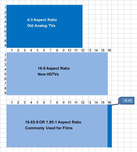
Figure 5.9
The problem is fitting the 4:3 and the cinematic film aspect ratio onto our HDTV. The simplest way is to take the 4:3 rectangle and fit it on the 16:9 rectangle. When you try this you can immediately understand why we see those black bars on the side. Similarly, when you watch a Blu-ray DVD that is supposed to be HD, you still get bars on the top and bottom. This is because the Blu-ray movie was recorded with the aspect ratio of 1.85:1. Figure 5.10 shows how the black bars appear when we try and fit a different aspect ratio on regular HDTV screen.

Figure 5.10
The reason these aspect ratios are brought up here is that you can immediately see one of the major uses for video scaling. Most HDTVs have a scaling function which will change the aspect ratio, but most of them employ simplistic scaling algorithms – nearest neighbor or bilinear – and so the resultant image is not very good.
Better results occur when the movie makers convert their film aspect ratio to a 16:9 aspect ratio – sometimes known as anamorphic widescreen. This is generally labeled on the DVD.
1.78:1
16:9
WIDESCREEN VERSION
5.4 Conclusion
Video scaling is probably one of the most common video processing techniques. It is used in a variety of applications – ranging from HDTV to medical, surveillance and conferencing systems. Done correctly, this is computationally intensive processing which has to be done at the video frame rate. It demands dedicated hardware and/or a fast FPGA to implement at acceptable quality and at fast frame rates.