
5.3. Tensor Voting in 2D
This section introduces the tensor voting framework in 2D. It begins by describing the original second-order representation and voting of [40]. Since the strictly second-order framework cannot handle structure discontinuities, first-order information has been added to the framework. Now tokens are encoded with second-order tensors and polarity vectors. These tokens propagate their information to their neighbors by casting first- and second-order votes. We demonstrate how all types of votes are derived from the same voting function and how voting fields are generated. Votes are accumulated at every token to infer the type of perceptual structure or structures going through it along with their orientation. Voting from token to token is called sparse voting. Then dense voting, during which votes are accumulated at all grid positions, can be performed to infer the saliency everywhere. This process allows the continuation of structures and the bridging of gaps. In 2D, perceptual structures can be curves, regions, and junctions, as well as their terminations, which are the endpoints of curves and the boundaries of regions. Finally, we present results on synthetic but challenging examples, including illusory contours.
5.3.1. Second-order representation and voting in 2D
The second-order representation is in the form of a second-order symmetric nonnegative definite tensor, which essentially indicates the saliency of each type of perceptual structure (curve, junction, or region in 2D) the token may belong to and its preferred normal and tangent orientations. Tokens cast second-order votes to their neighbors according to the tensors they are associated with.
Second-order representation
A 2D, symmetric, nonnegative definite, second-order tensor can be viewed as a 2 x 2 matrix, or equivalently an ellipse. Intuitively, its shape indicates the type of structure represented and its size the saliency of this information. The tensor can be decomposed as in the following equation:
Equation 5.1
![]()
where λi are the eigenvalues in decreasing order and êi are the corresponding eigenvectors (see also Figure 5.4). Note that the eigenvalues are nonnegative, since the tensor is nonnegative definite. The first term in (5.1) corresponds to a degenerate, elongated ellipsoid, termed hereafter the stick tensor, that indicates an elementary curve token with ê1 as its curve normal. The second term corresponds to a circular disk, termed the ball tensor, that corresponds to a perceptual structure that has no preference of orientation or to a location where multiple orientations coexist. The size of the tensor indicates the certainty of the information represented by it. For instance, the size of the stick component (λ1 - λ2) indicates curve saliency.
Figure 5.4. Decomposition of a 2D second-order, symmetric tensor into its stick and ball components.

Based on the above, an elementary curve with normal ![]() is represented by a stick tensor parallel to the normal, while an unoriented token is represented by a ball tensor. Note that curves are represented by their normals and not their tangents for reasons that become apparent in higher dimensions. See Table 5.1 for how oriented and unoriented inputs are encoded and the equivalent ellipsoids and quadratic forms.
is represented by a stick tensor parallel to the normal, while an unoriented token is represented by a ball tensor. Note that curves are represented by their normals and not their tangents for reasons that become apparent in higher dimensions. See Table 5.1 for how oriented and unoriented inputs are encoded and the equivalent ellipsoids and quadratic forms.
| Input | Second-order tensor | Eigenvalues | Quadratic form |
|---|---|---|---|
 | λ1 = 1, λ2 = 0 | ||
 | λ1 = λ2 = 1 |
Second-order voting
Now that the inputs, oriented or unoriented, have been encoded with tensors, we examine how the information they contain is propagated to their neighbors. The question we want to answer is: assuming that a token at O with normal ![]() and a token at P belong to the same smooth perceptual structure, what information should the token at O cast at P? We first answer the question for the case of a voter with a pure stick tensor and show how all other cases can be derived from it. We claim that in the absence of other information, the are of the osculating circle (the circle that shares the same normal as a curve at the given point) at O that goes through P is the most likely smooth path, since it maintains constant curvature. The center of the circle is denoted by C in Figure 5.5. In case of straight continuation from O to P, the osculating circle degenerates to a straight line. Similar use of primitive circular arcs can also be found in [50, 56, 55, 73].
and a token at P belong to the same smooth perceptual structure, what information should the token at O cast at P? We first answer the question for the case of a voter with a pure stick tensor and show how all other cases can be derived from it. We claim that in the absence of other information, the are of the osculating circle (the circle that shares the same normal as a curve at the given point) at O that goes through P is the most likely smooth path, since it maintains constant curvature. The center of the circle is denoted by C in Figure 5.5. In case of straight continuation from O to P, the osculating circle degenerates to a straight line. Similar use of primitive circular arcs can also be found in [50, 56, 55, 73].
Figure 5.5. Second-order vote cast by a stick tensor located at the origin.

As shown in Figure 5.5, the second-order vote is also a stick tensor and has a normal lying along the radius of the osculating circle at P. What remains to be defined is the magnitude of the vote. According to the Gestalt principles, it should be a function of proximity and smooth continuation. The influence from a token to another should attenuate with distance, to minimize interference from unrelated tokens, and with curvature, to favor straight continuation over curved alternatives when both exist. Moreover, no votes are cast if the receiver is at an angle larger than 45° with respect to the tangent of the osculating circle at the voter. Similar restrictions on the fields appear also in [19, 73, 36]. The saliency decay function we have selected has the following form:
Equation 5.2
![]()
where s is the are length OP, k is the curvature, c controls the degree of decay with curvature, and σ is the scale of voting, which determines the effective neighborhood size. The parameter c is a function of the scale and is optimized to make the extension of two orthogonal line segments to form a right angle equally likely to the completion of the contour with a rounded corner [15]. Its value is given by ![]() . Scale essentially controls the range within which tokens can influence other tokens. The saliency decay function has infinite extend, but for practical reasons it is cropped at a distance where the votes cast become insignificant. For instance, the field can be defined up to the extend that vote strength becomes less than 1% of the voter's saliency. The scale of voting can also be viewed as a measure of smoothness. A large scale favors long-range interactions and enforces a higher degree of smoothness, aiding noise removal at the same time, while a small scale makes the voting process more local, thus preserving details. Note that σ is the only free parameter in the system.
. Scale essentially controls the range within which tokens can influence other tokens. The saliency decay function has infinite extend, but for practical reasons it is cropped at a distance where the votes cast become insignificant. For instance, the field can be defined up to the extend that vote strength becomes less than 1% of the voter's saliency. The scale of voting can also be viewed as a measure of smoothness. A large scale favors long-range interactions and enforces a higher degree of smoothness, aiding noise removal at the same time, while a small scale makes the voting process more local, thus preserving details. Note that σ is the only free parameter in the system.
The 2D, second-order stick voting field for a unit stick voter located at the origin and aligned with the z-axis can be defined as follows as a function of the distance l between the voter and receiver and the angle θ, which is the angle between the tangent of the osculating circle at the voter and the line going through the voter and receiver (see Figure 5.5).
Equation 5.3
The votes are also stick tensors. For stick tensors of arbitrary size, the magnitude of the vote is given by (5.2) multiplied by the the size of the stick λ1 - λ2. The ball voting field is formally defined in Section 5.3.3. It can be derived from the second-order stick voting field It is used for voting tensors that have nonzero ball components and contain a tensor at every position that expresses the orientation preference and saliency of the receiver of a vote cast by a ball tensor. For arbitrary ball tensors, the magnitude of the votes has to be multiplied by λ2.
The voting process is identical whether the receiver contains a token or not, but we use the term sparse voting to describe a pass of voting where votes are cast to locations that contain tokens only, and the term dense voting for a pass of voting from the tokens to all locations within the neighborhood regardless of the presence of tokens. Receivers accumulate the votes cast to them by tensor addition.
Sensitivity to Scale
The scale of the voting field is the single critical parameter of the framework. Nevertheless, the sensitivity to it is low. Similar results should be expected for similar values of scale, and small changes in the output are associated with small changes of scale. We begin analyzing the effects of scale with simple synthetic data for which ground truth can be easily computed. The first example is a set of unoriented tokens evenly spaced on the periphery of a circle of radius 100 (see Figure 5.6a). The tokens are encoded as ball tensors, and tensor voting is performed to infer the most types of structures they form, which are always detected as curves, and their preferred orientations. The theoretic values for the tangent vector at each location can be calculated as [-sin(θ) cos(θ)]T.
Figure 5.6. Inputs for quantitative estimation of orientation errors as scale varies.

Table 5.2 reports the angular error in degrees between the ground-truth tangent orientation at each of the 72 locations and the orientation estimated by tensor voting. (Note that the values on the table are for σ2.) The second example in Figure 5.6b is a set of unoriented tokens lying at equal distances on a square of side 200. After voting, the junctions are detected due to their high ball saliency and the angular error between the ground truth, and the estimated tangent at each curve inlier is reported in Table 5.2. The extreme scale values, especially the larger ones, used here are beyond the range that is typically used in the other experiments presented in this chapter. A σ2 value of 50 corresponds to a voting neighborhood of I6, while a σ2 of 5000 corresponds to a neighborhood of I52. An observation from these simple experiments is that, as scale increases, each token receives more votes, leading to a better approximation of the circle by the set of points, while too much influence from the other sides of the square rounds its corners, causing an increase in the reported errors.
| σ2 | Angular error for circle (degrees) | Angular error for square (degrees) |
|---|---|---|
| 50 | 1.01453 | 1.11601e-007 |
| 100 | 1.14193 | 0.138981 |
| 200 | 1.11666 | 0.381272 |
| 300 | 1.04043 | 0.548581 |
| 400 | 0.974826 | 0.646754 |
| 500 | 0.915529 | 0.722238 |
| 750 | 0.813692 | 0.8893 |
| 1000 | 0.742419 | 1.0408 |
| 2000 | 0.611834 | 1.75827 |
| 3000 | 0.550823 | 2.3231 |
| 4000 | 0.510098 | 2.7244 |
| 5000 | 0.480286 | 2.98635 |
A different simple experiment demonstrating the stability of the results with respect to large scale variations is shown in Figure 5.7. The input consists of a set of unoriented tokens from a hand-drawn curve. Approximately half the points of the curve have been randomly removed from the data set, and the remaining points where spaced apart by 3 units of distance. Random outliers whose coordinates follow a uniform distribution have been added to the data. The I66 inliers and the 300 outliers are encoded as ball tensors, and tensor voting is performed with a wide range of scales. The detected inliers at a few scales are shown in Figure 5.7b-d. At the smallest scales, isolated inliers do not receive enough support to appear as salient, but as scale increases, the output becomes stable. In all cases, outliers are successfully removed. Table 5.3 shows the curve saliency of an inlier A and that of an outlier B as the scale varies. (Note that the values on the table again are for σ2.) Regardless of the scale, the saliency of A is always significantly larger than that of B, making the selection of a threshold that separates inliers from outliers trivial.
Figure 5.7. Noisy input for inlier/outlier saliency comparison.
5.3.2. First-order representation and voting in 2D
In this section, the need for integrating first-order information into the framework is justified. The first-order information is conveyed by the polarity vector that encodes the likelihood of the token being on the boundary of a perceptual structure. Such boundaries in 2D are the endpoints of curves and the end-curves of regions. The direction of the polarity vector indicates the direction of the inliers of the perceptual structure whose potential boundary is the token under consideration. The generation of first-order votes is shown based on the generation of second-order votes.
First-order representation
To illustrate the significance of adding the polarity vectors to the original framework as presented in [40], consider the contour depicted in Figure 5.8a, keeping in mind that we represent curve elements by their normals. The contour consists of a number of points, such as D, that can be considered "smooth inliers," since they can be inferred from their neighbors under the constraint of good continuation. Consider point A, which is an orientation discontinuity where two smooth segments of the contour intersect. A can be represented as having both curve normals simultaneously. This is a second-order discontinuity that is described in the strictly second-order framework by the presence of a salient ball component in the tensor structure. The ball component of the second-order tensor captures the uncertainty of orientation, with its size indicating the likelihood that the location is a junction. On the other hand, the endpoints B and C of the contour are smooth continuations of their neighbors in the sense that their normals do not differ significantly from those of the adjacent points.
Figure 5.8. Curves with orientation discontinuities at A and A' and endpoints B and C. The latter cannot be represented with second-order tensors.

The same is true for their tensors as well. Therefore, they cannot be discriminated from points B' and C' in Figure 5.8b. The property that makes these pairs of points very different is that B and C are terminations of the curve in Figure 5.8a, while their counterparts are not.
The second-order representation is adequate to describe locations where the orientation of the curve varies smoothly and locations where the orientation of the curve is discontinuous, which are second-order discontinuities. The termination of a perceptual structure is a first-order property and is handled by the first-order augmentation to the representation. Polarity vectors are vectors that are directed toward the direction where the majority of the neighbors of a perceptual structure are, and whose magnitude encodes the saliency of the token as a potential termination of the structure. The magnitude of these vectors, termed polarity hereafter, is locally maximum for tokens whose neighbors lie on one side of the half-space defined by the polarity vector. In the following sections, the way first-order votes are cast and collected to infer polarity and structure terminations is shown.
First-order voting
Now, we turn our attention to the generation of first-order votes. Note that the first-order votes are cast according to the second-order information of the voter. As shown in Figure 5.9, the first-order vote cast by a unitary stick tensor at the origin is tangent to the osculating circle, the smoothest path between the voter and receiver. Its magnitude, since nothing suggests otherwise, is equal to that of the second-order vote according to (5.2). The first-order voting field for a unit stick voter aligned with the z-axis is
Equation 5.4
![]()
Figure 5.9. Second- and first-order votes cast by a stick tensor located at the origin

Note that tokens are cast first- and second-order votes based on their second-order information only. This occurs because polarity vectors have to be initialized to zero, since no assumption about structure terminations is available. Therefore, first-order votes are computed based on the second-order representation, which can be initialized (in the form of ball tensors) even with no information other than the presence of a token.
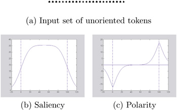
A simple illustration of how first- and second-order votes can be combined to infer curves and their endpoints in 2D appears in Figure 5.10. The input consists of a set of colinear, unoriented tokens, which are encoded as ball tensors. The tokens cast votes to their neighbors and collect the votes cast to them. The accumulated saliency can be seen in Figure 5.10b, where the dashed lines mark the limits of the input. The interior points of the curve receive more support and are more salient than those close to the endpoints. Since second-order voting is an excitatory process, locations beyond the end-points are also compatible with the inferred line and receive consistent votes from the input tokens. Detection of the endpoints based on the second-order votes is virtually impossible, since there is no systematic way of selecting a threshold that guarantees that the curve will not extend beyond the last input tokens. The strength of the second-order aspect of the framework lies in the ability to extrapolate and fill in gaps caused by missing data. The accumulated polarity can be seen in Figure 5.10c. The endpoints appear clearly as maxima of polarity. The combination of saliency and polarity al lows us to infer the curve and terminate it at the correct points. See Section 5.3.4 for a complete analysis of structure inference in 2D.
Figure 5.10. Accumulated saliency and polarity for a simple input.
5.3.3. Voting fields
In this section, we show how votes from ball tensors can be derived with the same saliency decay function and how voting fields can be computed to reduce the computational cost of calculating each vote according to (5.2). Finally, we show how the votes cast by an arbitrary tensor can be computed given the voting fields.
The second-order stick voting field contains at every position a tensor that is the vote cast there by a unitary stick tensor located at the origin and aligned with the y-axis. The shape of the field in 2D can be seen in the upper part of Figure 5.11a. Depicted at every position is the eigenvector corresponding to the largest eigenvalue of the second order tensor contained there. Its size is proportional to the magnitude of the vote. To compute a vote cast by an arbitrary stick tensor, we need to align the field with the orientation of the voter and multiply the saliency of the vote that coincides with the receiver by the saliency of the arbitrary stick tensor, as in Figure 5.11b.
Figure 5.11. Voting fields in 2D and alignment of the stick field with the data for vote generation.
The ball voting field can be seen in the lower part of Figure 5.11a. The ball tensor has no preference of orientation, but still can cast meaningful information to other locations. The presence of two proximate unoriented tokens, the voter and the receiver, indicates a potential curve going through the two tokens. The ball voting fields allow us to infer preferred orientations from unoriented tokens, thus minimizing initialization requirements.
The derivation of the ball voting field B(P) from the stick voting field can be visualized as follows: the vote at P from a unitary ball tensor at the origin O is the integration of the votes of stick tensors that span the space of all possible orientations. In 2D, this is equivalent to a rotating stick tensor that spans the unit circle at O. The 2D ball field can be derived from the stick field S(P), according to
Equation 5.5
![]()
where Rθ is the rotation matrix to align S with ê1, the eigenvector corresponding to the maximum eigenvalue (the stick component), of the rotating tensor at P.
In practice, the integration is approximated by tensor addition (see also Figure 5.12):
Equation 5.6

Figure 5.12. Tensor addition in 2D. Purely stick tensors result only from the addition of parallel stick tensors and purely ball tensors from the addition of ball tensors or orthogonal stick tensors.

where V is the accumulated vote and ![]() are the stick votes, in vector form (which is equivalent, since a stick tensor has only one nonzero eigenvalue and can be expressed as the outer product of its only significant eigenvector), from O to P cast by the stick tensors i ∊ [0, 2π) that span the unit circle. Normalization has to be performed in order to make the energy emitted by a unitary ball equal to that of a unitary stick. As a result of the integration, the second-order ball field does not contain purely stick or purely ball tensors, but arbitrary second-order symmetric tensors. The field is radially symmetric, as expected, since the voter has no preferred orientation.
are the stick votes, in vector form (which is equivalent, since a stick tensor has only one nonzero eigenvalue and can be expressed as the outer product of its only significant eigenvector), from O to P cast by the stick tensors i ∊ [0, 2π) that span the unit circle. Normalization has to be performed in order to make the energy emitted by a unitary ball equal to that of a unitary stick. As a result of the integration, the second-order ball field does not contain purely stick or purely ball tensors, but arbitrary second-order symmetric tensors. The field is radially symmetric, as expected, since the voter has no preferred orientation.
The 2D first-order stick voting field is a vector field, which at every position holds a vector that is equal in magnitude to the stick vote that exists in the same position in the fundamental second-order stick voting field, but is tangent to the smooth path between the voter and receiver instead of normal to it. The first-order ball voting field can be derived as in (5.5) by substituting the first-order stick field for the second-order stick field and performing vector instead of tensor addition when integrating the votes at each location.
All voting fields defined here, both first- and second-order, as well as all other fields in higher dimensions, are functions of the position of the receiver relative to the voter, the tensor at the voter, and a single parameter: the scale of the saliency decay function. After these fields have been precomputed at the desired resolution, computing the votes cast by any second-order tensor is reduced to a few look-up operations and linear interpolation. Voting takes place in a finite neighborhood within which the magnitude of the votes cast remains significant. For example, we can find the maximum distance smax from the voter at which the vote cast will have 1% of the voter's saliency, as follows:
Equation 5.7
![]()
The size of this neighborhood is obviously a function of the scale σ. As described in Section 5.3.1, any tensor can be decomposed into the basis components (stick and ball in 2D) according to its eigensystem. Then, the corresponding fields can be aligned with each component. Votes are retrieved by simple look-up operations, and their magnitude is multiplied by the corresponding saliency. The votes cast by the stick component are multiplied by λ1 - λ2, and those of the ball component by λ2
5.3.4. Vote analysis
Votes are cast from token to token and accumulated by tensor addition in the case of the second-order votes, which are in general arbitrary second-order tensors, and by vector addition in the case of the first-order votes, which are vectors.
Analysis of second-order votes
Analysis of the second-order votes can be performed once the eigensystem of the accumulated second-order 2 × 2 tensor has been computed. Then the tensor can be decomposed into the stick and ball components:
Equation 5.8
![]()
where ![]() is a stick tensor, and
is a stick tensor, and ![]() +
+ ![]() is a ball tensor. The following cases have to be considered. If λ1
» λ2, this indicates certainty of one normal orientation; therefore, the token most likely belongs on a curve that has the estimated normal at that location. If λ1 ≈ λ2, the dominant component is the ball and there is no preference of orientation, either because all orientations are equally likely or because multiple orientations coexist at the location. This indicates either a token that belongs to a region, which is surrounded by neighbors from the same region from all directions, or a junction where two or more curves intersect and multiple curve orientations are present simultaneously (see Figure 5.13). Junctions can be discriminated from region tokens, since their saliency is a distinct, local maximum of λ2, whereas the saliency of region inliers is more evenly distributed. An outlier receives only inconsistent votes, so both eigenvalues are small.
is a ball tensor. The following cases have to be considered. If λ1
» λ2, this indicates certainty of one normal orientation; therefore, the token most likely belongs on a curve that has the estimated normal at that location. If λ1 ≈ λ2, the dominant component is the ball and there is no preference of orientation, either because all orientations are equally likely or because multiple orientations coexist at the location. This indicates either a token that belongs to a region, which is surrounded by neighbors from the same region from all directions, or a junction where two or more curves intersect and multiple curve orientations are present simultaneously (see Figure 5.13). Junctions can be discriminated from region tokens, since their saliency is a distinct, local maximum of λ2, whereas the saliency of region inliers is more evenly distributed. An outlier receives only inconsistent votes, so both eigenvalues are small.
Figure 5.13. Salient ball tensors at regions and junctions.

Analysis of first-order votes
Vote collection for the first-order case is performed by vector addition. The accumulated result is a vector whose direction points to a weighted center of mass from which votes are cast, and whose magnitude encodes polarity. Since the first-order votes are also weighted by the saliency of the voters and attenuate with distance and curvature, their vector sum points to the direction from which the most salient contributions were received. A relatively low polarity indicates a token that is in the interior of a curve or region, therefore surrounded by neighbors whose votes cancel out each other. On the other hand, a high polarity indicates a token that is on or close to a boundary, thus receiving votes from only one side with respect to the boundary, at least locally. The correct boundaries can be extracted as maxima of polarity along the direction of the polarity vector. See the region of Figure 5.14, where the votes received at interior points cancel each other out, while the votes at boundary points reinforce each other resulting in a large polarity vector there. Table 5.4 illustrates how tokens can be characterized using the collected first- and second-order information.
Figure 5.14. First-order votes received at region inliers and boundaries.

| 2D feature | Saliency | Second-order tensor orientation | Polarity | Polarity vector |
|---|---|---|---|---|
| curve interior | high λ1 - λ2 | normal: ê1 | low | - |
| curve endpoint | high λ1 - λ2 | normal: ê1 | high | parallel to ê2 |
| region interior | high λ2 | - | low | - |
| region boundary | high λ2 | - | high | normal to boundary |
| junction | locally max λ2 | - | low | - |
| outlier | low | - | low | - |
Dense structure extraction
In order to extract dense structures based on the sparse set of tokens, an additional step is performed. Votes are collected at every location to determine where salient structures exist. The process of collecting votes at all locations regardless of whether they contain an input token or not is called dense voting. The tensors at every location are decomposed, and saliency maps are built. In 2D, there are two types of saliency that need to be considered: stick and ball saliency. Figure 5.15 shows an example where curve and junction saliency maps are built from a sparse set of oriented tokens.
Figure 5.15. Saliency maps in 2D (darker regions have higher saliency).

Curve extraction is performed as a marching process, during which curves are grown starting from seeds. The most salient unprocessed curve token is selected as the seed, and the curve is grown following the estimated normal. The next point is added to the curve with subpixel accuracy as the zero-crossing of the first derivative of saliency along the curve's tangent. Even though saliency values are available at discrete grid positions, the locations of the zero-crossings of the first derivative of saliency can be estimated with subpixel accuracy by interpolation. In practice, to reduce the computational cost of casting unnecessary votes, votes are collected only at grid points toward which the curve can grow, as indicated by the normal of the last point added. As the next point is added to the curve, following the path of maximum saliency, new grid points where saliency has to be computed are determined. Endpoints are critical, since they indicate where the curve should stop.
Regions can be extracted via their boundaries. As described previously, region boundaries can be detected based on their high region saliency and high polarity. Then, they are used as inputs to the curve extraction process described in the previous paragraph. Junctions are extracted as local maxima of the junction saliency map. This is the simplest case because junctions are isolated in space. Examples of the structure extraction processes described here are presented in the following subsection.
5.3.5. Results in 2D
In this section, we present examples of 2D perceptual grouping using the tensor voting framework. Figure 5.16a shows a data set that contains a number of fragmented sinusoidal curves represented by unoriented points contaminated by a large number of outliers. Figure 5.16b shows the output after tensor voting. Curve inliers are colored gray, endpoints black, while junctions appear as gray squares. All the noise has been removed, and the curve segments have been correctly detected and their endpoints and junctions labeled.
Figure 5.16. Curve, endpoint, and junction extraction from a noisy data set with sinusoidal curves.

The example in Figure 5.17 illustrates the detection of regions and curves. The input consists of a cardioid, represented by a set of unoriented points, and two quadratic curves, also represented as sets of unoriented points, contaminated by random uniformly distributed noise (Figure 5.17a). Figures 5.17b-d show the detected region inliers, region boundaries, and curve in-liers respectively. Note that some points, where the curves and the cardioid overlap, have been detected as both curve and region inliers.
Figure 5.17. Region and curve extraction from noisy data.

5.3.6. Illusory contours
An interesting phenomenon is the grouping of endpoints and junctions to form illusory contours. Kanizsa [29] demonstrated the universal and unambiguous perception of illusory contours caused by the alignment of endpoints, distant line segments, junctions, and corners; [19, 13, 14] developed computational models for the inference of illusory contours and point out the differences between them and regular contours. Illusory contours are always convex, and when they are produced by endpoints, their formation occurs in the orthogonal direction of the contours whose endpoints give rise to the illusory ones. A perception of an illusory contour is strong in the lower part of Figure 5.18a, while no contour is formed in the upper part.
Figure 5.18. Illusory contours are perceived when they are convex (a). The single-sided field used for illusory contour inference. P denotes the polarity vector of the voting endpoint.

The capability to detect endpoints can be put to use for the inference of illusory contours. Figure 5.19a shows a set of line segments whose extensions converge to the same point and whose endpoints form an illusory circle. The segments consist of unoriented points, which are encoded as ball tensors, and propagate first- and second-order votes to their neighbors. The endpoints can be detected based on their high polarity values. They can be seen in Figure 5.19b along with the polarity vectors. The direction of the polarity vectors determines the side of the half-plane where the endpoint should cast second-order votes to ensure that the inferred illusory contours are convex. These votes are cast using a special field, shown in Figure 5.18b. This field is single-sided and is orthogonal to the regular field. Alternatively, the endpoint voting field can be viewed as the positive side of the fundamental stick field rotated by 90 degrees. A dense contour, a circle, is inferred after these votes have been collected and analyzed, as in the previous subsection (Figure 5.19c). Note that first-order fields can be defined in a similar way. An aspect of illusory contour inference that requires further investigation is a mechanism for deciding whether to employ regular voting fields to connect fragmented curves or to employ the orthogonal fields to infer illusory contours.
Figure 5.19. Illusory contour inference from endpoints of linear segments
