
Open Shortest Path First (OSPF) was developed by the Internet Engineering Task Force (IETF) as a replacement for the problematic RIP and is now the IETF-recommended Interior Gateway Protocol (IGP). OSPF is a link-state protocol that, as the name implies, uses Dijkstra’s Shortest Path First (SPF) algorithm and that is open—that is, it isn’t proprietary to any vendor or organization. OSPF has evolved through several RFCs, all of which were written by John Moy. Version 1 of the protocol was specified in RFC 1131; this version never progressed beyond the experimental stage. Version 2, which is still the current version for IPv4, was first specified in RFC 1247, and the most recent specification is RFC 2328.
Like all link-state protocols, OSPF’s major advantages over distance vector protocols are fast reconvergence, scalability to much larger networks, and less susceptibility to bad routing information. Other features of OSPF are
The use of areas, which reduces the protocol’s impact on CPU and memory, contains the flow of routing protocol traffic, and makes possible the construction of hierarchical network topologies
Fully classless behavior, eliminating such classful problems as discontiguous subnets
Support of classless route table lookups, VLSM, and supernetting for efficient address management
A dimensionless, arbitrary metric
Equal-cost load balancing for more efficient use of multiple paths[1]
The use of reserved multicast addresses to reduce the impact on non-OSPF–speaking devices
Support of authentication for more secure routing
The use of route tagging for the tracking of external routes
OSPF also has the capability of supporting Type of Service (TOS) routing, although it was never widely implemented. RFC 2328 has deleted the TOS routing option for this reason.
Operation of OSPF[2]
At a very high level, the operation of OSPF is easily explained:
OSPF-speaking routers send Hello packets out all OSPF-enabled interfaces. If two routers sharing a common data link agree on certain parameters specified in their respective Hello packets, they will become neighbors.
Adjacencies, which can be thought of as virtual point-to-point links, are formed between some neighbors. OSPF defines several network types and several router types. The establishment of an adjacency is determined by the types of routers exchanging Hellos and the type of network over which the Hellos are exchanged.
Each router sends link-state advertisements (LSAs) over all adjacencies. The LSAs describe all of the router’s links, or interfaces, the router’s neighbors, and the state of the links. These links might be to stub networks (networks with no other router attached), to other OSPF routers, to networks in other areas, or to external networks (networks learned from another routing process). Because of the varying types of link-state information, OSPF defines multiple LSA types.
Each router receiving an LSA from a neighbor records the LSA in its link-state database and sends a copy of the LSA to all of its other neighbors.
By flooding LSAs throughout an area, all routers will build identical link-state databases.
When the databases are complete, each router uses the SPF algorithm to calculate a loop-free graph describing the shortest (lowest cost) path to every known destination, with itself as the root. This graph is the SPF tree.
Each router builds its route table from its SPF tree.[3]
When all link-state information has been flooded to all routers in an area and neighbors have verified that their databases are identical—that is, the link-state databases have been synchronized—and the route tables have been built, OSPF is a quiet protocol. Hello packets are exchanged between neighbors as keepalives, and LSAs are retransmitted every 30 minutes. If the network topology is stable, no other activity should occur.
Before any LSAs can be sent, OSPF routers must discover their neighbors and establish adjacencies. The neighbors will be recorded in a neighbor table, along with the link (interface) on which each neighbor is located and which contains other information necessary for the maintenance of the neighbor (Example 8-1).
Example 8-1. The neighbor table records all OSPF-speaking neighbors.
Monet#show ip ospf neighbor
Neighbor ID    Pri   State    Dead Time    Address        Interface
192.168.30.70    1   FULL/DR  00:00:34     192.168.17.73  Ethernet0
192.168.30.254   1   FULL/DR  00:00:34     192.168.32.2   Ethernet1
192.168.30.70    1   FULL/BDR 00:00:34     192.168.32.4   Ethernet1
192.168.30.30    1   FULL/ -  00:00:33     192.168.17.50  Serial0.23
192.168.30.10    1   FULL/ -  00:00:32     192.168.17.9   Serial1
192.168.30.68    1   FULL/ -  00:00:39     192.168.21.134 Serial2.824
192.168.30.18    1   FULL/ -  00:00:30     192.168.21.142 Serial2.826
192.168.30.78    1   FULL/ -  00:00:36     192.168.21.170 Serial2.836
The tracking of other OSPF routers requires that each router have a Router ID, an IP address by which the router is uniquely identified within the OSPF domain. Cisco routers derive their Router IDs by the following means:
If the Router ID has been manually configured using the router-id command, that Router ID is used.
If no Router ID has been manually configured, the router chooses the numerically highest IP address on any of its loopback interfaces.
If no loopback interfaces are configured with IP addresses, the router chooses the numerically highest IP address on any of its physical interfaces. The interface from which the Router ID is taken does not have to be running OSPF.
Using addresses associated with loopback interfaces has two advantages:
The loopback interface is more stable than any physical interface. It is active when the router boots up, and it only fails if the entire router fails.
The network administrator has more leeway in assigning predictable or recognizable addresses as the Router IDs.
The Cisco OSPF will continue to use a Router ID learned from a physical interface even if the interface subsequently fails or is deleted (see “Case Study: Setting Router IDs with Loopback Interfaces,” later in this chapter). Therefore, the stability of a loopback interface is only a minor advantage. The primary benefit is the ability to control the Router ID.
The OSPF router begins a neighbor relationship by advertising its Router ID in Hello packets.
The Hello protocol serves several purposes:
It is the means by which neighbors are discovered.
It advertises several parameters on which two routers must agree before they can become neighbors.
Hello packets act as keepalives between neighbors.
It ensures bidirectional communication between neighbors.
It elects Designated Routers (DRs) and Backup Designated Routers (BDRs) on Broadcast and Nonbroadcast Multiaccess (NBMA) networks.
OSPF-speaking routers periodically send a Hello packet out each OSPF-enabled interface. This period is known as the HelloInterval and is configured on a per interface basis. Cisco uses a default HelloInterval of 10 seconds for broadcast networks and 30 seconds for non-broadcast; the value can be changed with the command ip ospf hello-interval. If a router has not heard a Hello from a neighbor within a period of time known as the RouterDeadInterval, it will declare the neighbor down. The Cisco default RouterDeadInterval is four times the HelloInterval and can be changed with the command ip ospf dead-interval.[4]
Each Hello packet contains the following information:
Router ID of the originating router.
Area ID of the originating router interface.
Address mask of the originating interface.
Authentication type and authentication information for the originating interface.
HelloInterval of the originating interface.
RouterDeadInterval of the originating interface.
Router Priority.
DR and BDR.
Five flag bits signifying optional capabilities.
Router IDs of the originating router’s neighbors. This list contains only routers from which Hellos were heard on the originating interface within the last RouterDeadInterval.
This section overviews the meaning and use of most of the information listed. Subsequent sections discuss the DR, BDR, and Router Priority, and illustrate the precise format of the Hello packet. When a router receives a Hello from a neighbor, it will verify that the Area ID, Authentication, Network Mask, HelloInterval, RouterDeadInterval, and Options values match the values configured on the receiving interface. If they do not, the packet is dropped and no adjacency is established.
If everything matches, the Hello packet is declared valid. If the ID of the originating router is already listed in the neighbor table for that receiving interface, the RouterDeadInterval timer is reset. If the Router ID is not listed, it is added to the neighbor table.
Whenever a router sends a Hello, it includes in the packet the Router IDs of all neighbors listed for the link on which the packet is to be transmitted. If a router receives a valid Hello in which it finds its own Router ID listed, the router knows that two-way communication has been established.
After two-way communication has been established, adjacencies may be established. However, as mentioned earlier, not all neighbors will become adjacent. Whether an adjacency is formed or not depends on the type of network to which the two neighbors are attached. Network types also influence the way in which OSPF packets are transmitted; therefore, before discussing adjacencies, it is necessary to discuss network types.
OSPF defines five network types:
Point-to-point networks
Broadcast networks
Nonbroadcast Multiaccess (NBMA) networks
Point-to-multipoint networks
Virtual links
Point-to-point networks, such as a T1, DS-3, or SONET link, connect a single pair of routers. Valid neighbors on point-to-point networks will always become adjacent. The destination address of OSPF packets on these networks will always be the reserved class D address 224.0.0.5, known as AllSPFRouters.[5]
Broadcast networks, such as Ethernet, Token Ring, and FDDI, might be better defined as broadcast multi-access networks to distinguish them from NBMA networks. Broadcast networks are multi-access in that they are capable of connecting more than two devices, and they are broadcast in that all attached devices can receive a single transmitted packet. OSPF routers on broadcast networks will elect a DR and a BDR, as described in the next section, “Designated Routers and Backup Designated Routers.” Hello packets are multicast with the AllSPFRouters destination address 224.0.0.5, as are all OSPF packets originated by the DR and BDR. The destination Media Access Control (MAC) identifier of the frames carrying these packets is 0100.5E00.0005. All other routers will multicast link-state update and link-state acknowledgment packets (described later) to the reserved class D address 224.0.0.6, known as AllDRouters. The destination MAC identifier of the frames carrying these packets is 0100.5E00.0006.
NBMA networks, such as X.25, Frame Relay, and ATM, are capable of connecting more than two routers but have no broadcast capability. A packet sent by one of the attached routers would not be received by all other attached routers. As a result, extra configuration might be necessary for routers on these networks to acquire their neighbors. OSPF routers on NBMA networks elect a DR and BDR, and all OSPF packets are unicast.
Point-to-multipoint networks are a special configuration of NBMA networks in which the networks are treated as a collection of point-to-point links. Routers on these networks do not elect a DR and BDR, and the OSPF packets are unicast to each known neighbor.
Virtual links, described in a later section, are special configurations that are interpreted by the router as unnumbered point-to-point networks. OSPF packets are unicast over virtual links.
In addition to these five network types, it should be noted that all networks fall into one of two more-general types:
Transit networks have two or more attached routers. They might carry packets that are “just passing through”—packets that were originated on and are destined for a network other than the transit network.
Stub networks have only a single attached router.[6] Packets on a stub network always have either a source or a destination address belonging to that network. That is, all packets were either originated by a device on the network or are destined for a device on the network. OSPF advertises host routes (routes with a mask of 255.255.255.255) as stub networks. Loopback interfaces are also considered stub networks and are advertised as host routes.[7]
Multiaccess networks present two problems for OSPF, relating to the flooding of LSAs (described in a later section):
The formation of an adjacency between every attached router would create many unnecessary LSAs. If n is the number of routers on a multiaccess network, there would be n(n – 1)/2 adjacencies (Figure 8-1). Each router would flood n – 1 LSAs for its adjacent neighbors, plus one LSA for the network, resulting in n2 LSAs originating from the network.
Flooding on the network itself would be chaotic and excessive. A router would flood an LSA to all its adjacent neighbors, which in turn would flood it to all their adjacent neighbors, creating many copies of the same LSA on the same network.
To prevent these problems, a DR is elected on multi-access networks. The DR has the following duties:
To represent the multi-access network and its attached routers to the rest of the OSPF area
To manage the flooding process on the multi-access network
The concept behind the DR is that the broadcast link itself is considered a “pseudonode,” or a virtual router. When the SPF tree is calculated, the link appears as a node and the routers attached to the link are attached to that node. The cost from an attached router to the pseudonode is the outgoing cost of that router’s interface to the broadcast link, but the cost from the pseudonode to any attached router is 0. This way, the overall path cost is not affected by the pseudonode.
Each router on the network forms an adjacency with the DR (Figure 8-2), which represents the pseudonode with a special Network LSA. Keep in mind that a router might be a DR on one of its attached multi-access networks, and it might not be the DR on another of its attached multi-access networks. In other words, the DR is a property of a router’s interface, not the entire router.

Figure 8-2. The DR represents the multi-access network. Other routers on the network will form adjacencies with the DR, not with each other.
A significant problem with the DR scheme as described so far is that if the DR fails, a new DR must be elected. New adjacencies must be established, and all routers on the network must synchronize their databases with the new DR (part of the adjacency-building process). While all this is happening, the network is unavailable for transit packets.
To prevent this problem, a BDR is elected in addition to the DR. All routers form adjacencies not only with the DR but also with the BDR. The DR and BDR also become adjacent with each other. If the DR fails, the BDR becomes the new DR. Because the other routers on the network are already adjacent with the BDR, network unavailability is minimized.
The election of the DR and BDR is triggered by the interface state machine, which is described in a later section. For the election process to function properly, the following preconditions must exist:
Each multi-access interface of each router has a Router Priority, which is an 8-bit unsigned integer ranging from 0 to 255. The default priority on Cisco routers is 1 and can be changed on a per multi-access-interface basis with the command ip ospf priority. Routers with a priority of 0 are ineligible to become the DR or BDR.
Hello packets include fields for the originating router to specify its Router Priority and for the IP addresses of the connected interfaces of the routers it considers the DR and BDR.
When an interface first becomes active on a multi-access network, it sets the DR and BDR to 0.0.0.0. It also sets a wait timer with a value equal to the RouterDeadInterval.
Existing interfaces on a multi-access network record the addresses of the DR and the BDR in the interface data structure, described in a later section.
The election procedure of the DR and BDR is as follows:
After two-way communication has been established with one or more neighbors, examine the Priority, DR, and BDR fields of each neighbor’s Hello. List all routers eligible for election (that is, routers with priority greater than 0 and whose neighbor state is at least two-way); all routers declaring themselves to be the DR (their own interface address is in the DR field of the Hello packet); and all routers declaring themselves to be the BDR (their own interface address is in the BDR field of the Hello packet). The calculating router will include itself on this list unless it is ineligible.
From the list of eligible routers, create a subset of all routers not claiming to be the DR (routers declaring themselves to be the DR cannot be elected BDR).
If one or more neighbors in this subset include its own interface address in the BDR field, the neighbor with the highest priority will be declared the BDR. In a tie, the neighbor with the highest Router ID will be chosen.
If no router in the subset claims to be the BDR, the neighbor with the highest priority will become the BDR. In a tie, the neighbor with the highest Router ID will be chosen.
If one or more of the eligible routers include their own address in the DR field, the neighbor with the highest priority will be declared the DR. In a tie, the neighbor with the highest Router ID will be chosen.
If no router has declared itself the DR, the newly elected BDR will become the DR.
If the router performing the calculation is the newly elected DR or BDR, or if it is no longer the DR or BDR, repeat steps 2 through 6.
In simpler language, when an OSPF router becomes active and discovers its neighbors, it checks for an active DR and BDR. If a DR and BDR exist, the router accepts them. If there is no BDR, an election is held in which the router with the highest priority becomes the BDR. If more than one router has the same priority, the one with the numerically highest Router ID wins. If there is no active DR, the BDR is promoted to DR and a new election is held for the BDR.
It should be noted that the priority can influence an election, but will not override an active DR or BDR. That is, if a router with a higher priority becomes active after a DR and BDR have been elected, the new router will not replace either of them. So the first two DR-eligible routers to initialize on a multiaccess network will become the DR and BDR.
After the DR and BDR have been elected, the other routers (known as DRothers) will establish adjacencies with the DR and BDR only. All routers continue to multicast Hellos to the AllSPFRouters address 224.0.0.5 so that they can track neighbors, but DRothers multicast update packets to the AllDRouters address 224.0.0.6. Only the DR and BDR will listen to this address; in turn, the DR will flood the updates to the DRothers on 224.0.0.5.
Note that if only one eligible router is attached to a multiaccess network, that router will become the DR and there will be no BDR. Any other routers will form adjacencies only with the DR. If none of the routers attached to a multi-access network are eligible, there will be no DR or BDR and no adjacencies will form. The neighbor states of all routers will remain two-way (explained later, in “Neighbor State Machine”).
The duties performed by the DR and BDR are described more fully in subsequent sections.
The essence of a link-state protocol is that it is concerned with links and the state of those links. Before Hellos can be sent, before adjacencies can be formed, and before LSAs can be sent, an OSPF router must understand its own links. A router’s interfaces are the means by which OSPF interprets links. As a result, when speaking of OSPF, it is not uncommon to hear the terms interface and link used synonymously. This section examines the data structure OSPF associates with each interface and the various states of an OSPF interface.
An OSPF router maintains a data structure for each OSPF-enabled interface. In Example 8-2, the command show ip ospf interface has been used to observe the components of an interface data structure.[8]
Example 8-2. The OSPF-specific data related to an interface can be observed with the command show ip ospf interface. In this example, the interface is attached to a point-to-point network type.
Renoir#show ip ospf interface Serial1.738
Serial1.738 is up, line protocol is up
   Internet Address 192.168.21.21/30, Area 7
   Process ID 1, Router ID 192.168.30.70, Network Type POINT_TO_POINT, Cost: 781
   Transmit Delay is 1 sec, State POINT_TO_POINT,
   Timer intervals configured, Hello 10, Dead 40, Wait 40, Retransmit 5
      Hello due in 00:00:07
   Neighbor Count is 1, Adjacent neighbor count is 1
      Adjacent with neighbor 192.168.30.77
   Message digest authentication enabled
      Youngest key id is 10
The components of the interface data structure are as follows:
IP Address and Mask—. This component is the configured address and mask of the interface. OSPF packets originated from this interface will have this source address. In Example 8-2, the address/mask pair is 192.168.21.21/30.
Area ID—. The area to which the interface, and the network to which it is attached, belong. OSPF packets originated from this interface will have this Area ID. In Example 8-2, the area ID is 7.
Process ID—. This Cisco-specific feature is not part of the open standard. Cisco routers are capable of running multiple OSPF processes and use the Process ID to distinguish them. The Process ID has no significance outside the router on which it is configured. In Example 8-2, the Process ID is 1.
Router ID—. In Example 8-2, the Router ID is 192.168.30.70.
Network Type—. The type of network to which the interface is connected: broadcast, point-to-point, NBMA, point-to-multipoint, or virtual link. In Example 8-2, the network type is point-to-point.[9]
Cost—. The outgoing cost for packets transmitted from this interface. Cost is the OSPF metric, expressed as an unsigned 16-bit integer in the range of 1 to 65535. Cisco uses a default cost of 108/BW, expressed in whole numbers, where BW is the configured bandwidth of the interface and 108 is the reference bandwidth. The interface in Example 8-2 has a configured bandwidth of 128K (not shown in the example), so the cost is 108/128K = 781.
The cost can be changed with the command ip ospf cost. This command is especially important when configuring Cisco routers in a multivendor environment. Another vendor, for example, might use a default cost of 1 on all interfaces (essentially making OSPF cost reflect hop counts). If all routers do not assign costs in the same manner, OSPF can route improperly, suboptimally, or in some other unexpected way.
The reference bandwidth of 108 creates a problem for some modern media with bandwidths higher than 100M (such as OC-3 or above and Gigabit Ethernet). 108/100M = 1, meaning that higher bandwidths calculate to a fraction of 1, which is not allowed. So any cost that is calculated to a fraction of 1 is rounded up to 1. However, this means that if your network consists of high-bandwidth links, all interfaces wind up with a cost of 1 and the calculated shortest paths become based on least router hops. To remedy this, Cisco provides the command auto-cost reference-bandwidth, which allows the default reference bandwidth to be changed.
Other components of the interface data structure are as follows:
InfTransDelay—. The seconds by which LSAs exiting the interface will have their ages incremented. In Example 8-2, this is displayed as Transmit Delay and is shown to be the Cisco default, 1 second. InfTransDelay can be changed with the command ip ospf transmit-delay.
State—. The functional state of the interface, which is described in the following section, “Interface State Machine.”
Router Priority—. This 8-bit unsigned integer in the range of 0 to 255 elects the DR and BDR. The priority is not displayed in Example 8-2 because the network type is point-to-point; no DR or BDR is elected on this network type. Example 8-3 shows another OSPF interface in the same router. This interface shows an attached network type of broadcast, so a DR and BDR are elected. The priority shown is 1, the Cisco default. The command ip ospf priority is used to change the Router Priority.
Example 8-3. This interface is attached to a broadcast network type, and the router is the DR on this network.
Renoir#show ip ospf interface Ethernet0
Ethernet0 is up, line protocol is up
   Internet Address 192.168.17.73/29, Area 0
   Process ID 1, Router ID 192.168.30.70, Network Type BROADCAST, Cost: 10
   Transmit Delay is 1 sec, State DR, Priority 1
   Designated Router (ID) 192.168.30.70, Interface address 192.168.17.73
   Backup Designated router (ID) 192.168.30.80, Interface address 192.168.17.74
   Timer intervals configured, Hello 10, Dead 40, Wait 40, Retransmit 5
      Hello due in 00:00:03
   Neighbor Count is 1, Adjacent neighbor count is 1
      Adjacent with neighbor 192.168.30.80 (Backup Designated Router)
   Message digest authentication enabled
      Youngest key id is 10
Designated Router—. The DR for the network to which the interface is attached is recorded both by its Router ID and by the address of the interface attached to the shared network. Note that no DR is displayed in Example 8-2; it will be displayed only for multi-access network types. In Example 8-3, the DR is 192.168.30.70. The address of its attached interface is 192.168.17.73. A look at the Router ID, the interface address, and the interface state shows that Renoir is the DR.
Backup Designated Router—. The BDR for the network to which the interface is attached is also recorded both by its Router ID and by the address of the attached interface. In Example 8-3, the BDR is 192.168.30.80, and its interface address is 192.168.17.74.
HelloInterval—. The period, in seconds, between transmissions of Hello packets on the interface. This period is advertised in Hello packets that are transmitted from the interface. Cisco uses a default of 10 seconds on broadcast networks and 30 seconds on non-broadcast networks, which can be changed with the command ip ospf hello-interval. Example 8-3 displays HelloInterval as Hello and shows that the default is being used.
RouterDeadInterval—. The period, in seconds, that the router will wait to hear a Hello from a neighbor on the network to which the interface is connected before declaring the neighbor down. The RouterDeadInterval is advertised in Hello packets transmitted from the interface. Cisco uses a default of four times the HelloInterval; the default can be changed with the command ip ospf dead-interval. Example 8-3 displays the RouterDeadInterval as Dead and shows that the default is being used.
Wait Timer—. The length of time the router will wait for a DR and BDR to be advertised in a neighbor’s Hello packet before beginning a DR and BDR selection. The period of the wait timer is the RouterDeadInterval. In Example 8-2, the wait time is irrelevant because the interface is attached to a point-to-point network; no DR or BDR will be used.
RxmtInterval—. The period, in seconds, the router will wait between retransmissions of OSPF packets that have not been acknowledged. Example 8-3 displays this period as retransmit and shows that the Cisco default of five seconds is being used. An interface’s RxmtInterval can be changed with the command ip ospf retransmit-interval.
Hello Timer—. A timer that is set to the HelloInterval. When it expires, a Hello packet is transmitted from the interface. Example 8-3 shows that the Hello timer will expire in three seconds.
Neighboring Routers—. A list of all valid neighbors (neighbors whose Hellos have been seen within the past RouterDeadInterval) on the attached network. Example 8-4 shows yet another interface on the same router. Here, five neighbors are known on the network, but only two are adjacent (the Router IDs of only the adjacent neighbors are displayed). As a DRother on this network, the router has established an adjacency only with the DR and the BDR, in keeping with the DR protocol.
Example 8-4. On this network, the router sees five neighbors but has only formed adjacencies with the DR and the BDR.
Renoir#show ip ospf interface Ethernet1
Ethernet1 is up, line protocol is up
   Internet Address 192.168.32.4/24, Area 78
   Process ID 1, Router ID 192.168.30.70, Network Type BROADCAST, Cost: 10
   Transmit Delay is 1 sec, State DROTHER, Priority 1
   Designated Router (ID) 192.168.30.254, Interface address 192.168.32.2
   Backup Designated router (ID) 192.168.30.80, Interface address 192.168.32.1
   Timer intervals configured, Hello 10, Dead 40, Wait 40, Retransmit 5
      Hello due in 00:00:01
   Neighbor Count is 5, Adjacent neighbor count is 2
      Adjacent with neighbor 192.168.30.80 (Backup Designated Router)
      Adjacent with neighbor 192.168.30.254 (Designated Router)
   Message digest authentication enabled
Youngest key id is 10AuType—. Describes the type of authentication used on the network. The authentication type may be Null (no authentication), Simple Password, or Cryptographic (Message Digest). Example 8-4 shows that Message Digest authentication is being used. If Null authentication is used, no authentication type or key information will be displayed when show ip ospf interface is invoked.
Authentication Key—. A 64-bit password if simple authentication has been enabled for the interface or a message digest key if Cryptographic authentication is used. Example 8-4 shows that the “youngest key ID” is 10. This alludes to the fact that Cryptographic authentication allows the configuration of multiple keys on an interface to ensure smooth and secure key changes.
Example 8-5 shows an interface that is connected to an NBMA network. Notice that the HelloInterval is 30 seconds, the default for NBMA, and that the RouterDeadInterval is at the default of four times the HelloInterval.
Example 8-5. This interface is attached to a NBMA Frame Relay network and is the BDR for this network.
Renoir#show ip ospf interface Serial3
Serial3 is up, line protocol is up
   Internet Address 192.168.16.41/30, Area 0
   Process ID 1, Router ID 192.168.30.105, Network Type NON_BROADCAST, Cost: 64
   Transmit Delay is 1 sec, State BDR, Priority 1
   Designated Router (ID) 192.168.30.210, Interface address 192.168.16.42
   Backup Designated router (ID) 192.168.30.105, Interface address 192.168.16.41
   Timer intervals configured, Hello 30, Dead 120, Wait 120, Retransmit 5
      Hello due in 00:00:08
   Neighbor Count is 1, Adjacent neighbor count is 1
      Adjacent with neighbor 192.168.30.210 (Designated Router)
It is worthwhile to spend some time comparing Example 8-2 through Example 8-5. All four interfaces are on the same router, yet on each network the router performs a different role. In each case, the interface state dictates the role of the OSPF router on a network. The next section describes the various interface states and the interface state machine.
An OSPF-enabled interface will transition through several states before it becomes fully functional. Those states are Down, Point-to-Point, Waiting, DR, Backup, DRother, and Loopback.
Down—. This is the initial interface state. The interface is not functional, all interface parameters are set to their initial values, and no protocol traffic is transmitted or received on the interface.
Point-to-Point—. This state is applicable only to interfaces connected to point-to-point, point-to-multipoint, and virtual link network types. When an interface transitions to this state, it is fully functional. It will begin sending Hello packets every HelloInterval and will attempt to establish an adjacency with the neighbor at the other end of the link.
Waiting—. This state is applicable only to interfaces connected to broadcast and NBMA network types. When an interface transitions to this state, it will begin sending and receiving Hello packets and will set the wait timer. The router will attempt to identify the network’s DR and BDR while in this state.
DR—. In this state, the router is the DR on the attached network and will establish adjacencies with the other routers on the multi-access network.
Backup—. In this state, the router is the BDR on the attached network, and will establish adjacencies with the other routers on the multi-access network.
DRother—. In this state, the router is neither the DR nor the BDR on the attached network. It will form adjacencies only with the DR and BDR, although it will track all neighbors on the network.
Loopback—. In this state, the interface is looped back via software or hardware. Although packets cannot transit an interface in this state, the interface address is still advertised in Router LSAs (described later) so that test packets can find their way to the interface.
Figure 8-3 shows the OSPF interface states and the input events that will cause a state transition. The input events are described in Table 8-1.
Figure 8-3. The OSPF interface state machine; see Table 8-1 for a description of input events (IEs).
Table 8-1. Input events for the interface state machine.
Description | |
|---|---|
IE1 | Lower-level protocols indicate that the network interface is operational. |
IE2 | Lower-level protocols indicate that the network interface is not operational. |
IE3 | Network management or lower-level protocols indicate that the interface is looped up. |
IE4 | Network management or lower-level protocols indicate that the interface is looped down. |
IE5 | A Hello packet is received in which either the originating neighbor lists itself as the BDR or the originating neighbor lists itself as the DR and indicates no BDR. |
IE6 | The wait timer has expired. |
IE7 | The router is elected as the DR for this network. |
IE8 | The router is elected as the BDR for this network. |
IE9 | The router has not been elected as the DR or BDR for this network. |
IE10 | A change has occurred in the set of valid neighbors on this network. This change may be one of the following:
|
The preceding section discussed a router’s relationship with the attached data link. Although a router’s interaction with other routers was discussed in the context of electing DRs and BDRs, the purpose of the DR election process is still to establish a relationship with a link. This section discusses a router’s relationship with the neighbors on the network. The ultimate purpose of the neighbor relationship is the formation of adjacencies over which to pass routing information.
An adjacency is established in four general phases:
Neighbor discovery.
Bidirectional communication. This communication is accomplished when two neighbors list each other’s Router IDs in their Hello packets.
Database synchronization. Database Description, Link State Request, Link State Update, and Link State Acknowledgement packets (described in a later section) are exchanged to ensure that both neighbors have identical information in their link-state databases. For the purposes of this process, one neighbor will become the master and the other will become the slave. As the name implies, the master will control the exchange of Database Description packets.
Full adjacency.
As previously discussed, neighbor relationships are established and maintained through the exchange of Hello packets. On broadcast and point-to-point network types, Hellos are multicast to AllSPFRouters (224.0.0.5). On NBMA, point-to-multipoint, and virtual link network types, Hellos are unicast to individual neighbors. The implication of unicasting is that the router must first learn of the existence of its neighbors either through manual configuration or an underlying mechanism such as Inverse ARP. The configuration of neighbors on these network types is covered in the appropriate sections.
Hellos are sent every HelloInterval on every network type, with one exception: On NBMA networks, a router will send Hellos to neighbors whose neighbor state is down every PollInterval. On Cisco routers, the default PollInterval is 120 seconds.
An OSPF router builds the Hello packets for each network using the information stored in the interface data structure of the attached interface. By sending the Hello packets containing this information, the router informs neighbors about itself. Likewise, for each neighbor the router will maintain a neighbor data structure consisting of the information learned from other routers’ Hello packets.
In Example 8-6, the command show ip ospf neighbor is used to observe some of the information in the neighbor data structure for a single neighbor.[10]
Example 8-6. An OSPF router describes each conversation with each neighbor by a neighbor data structure.
Seurat#show ip ospf neighbor 10.7.0.1
 Neighbor 10.7.0.1, interface address 10.8.1.2
    In the area 0 via interface Ethernet0/0
    Neighbor priority is 1, State is FULL, 6 state changes
    DR is 10.8.1.1 BDR is 10.8.1.2
    Options is 0x52
    LLS Options is 0x1 (LR)
    Dead timer due in 00:00:30
    Neighbor is up for 09:55:04
    Index 1/3, retransmission queue length 0, number of retransmission 1
    First 0x0(0)/0x0(0) Next 0x0(0)/0x0(0)
    Last retransmission scan length is 1, maximum is 1
    Last retransmission scan time is 0 msec, maximum is 0 msec
Actually, the data structure records more information about each neighbor than is shown in the example.[11] The components of the neighbor data structure are as follows:
Neighbor ID—. The router ID of the neighbor. In Example 8-6, the neighbor ID is 10.7.0.1.
Neighbor IP Address—. The IP address of the neighbor’s interface attached to the network. When OSPF packets are unicasted to the neighbor, this address will be the destination address. In Example 8-6, the neighbor’s IP address is 10.8.1.2.
Area ID—. For two routers to become neighbors, the Area ID carried in a received Hello packet must match the Area ID of the receiving interface. The Area ID of the neighbor in Example 8-6 is 0 (0.0.0.0).
Interface—. The interface attached to the network on which the neighbor is located. In Example 8-6, the neighbor is reached via Ethernet0/0.
Neighbor Priority—. This component is the Router Priority of the neighbor, as advertised in the neighbor’s Hello packets. The priority is used in the DR/BDR election process. The neighbor in Example 8-6 has a priority of 1, the Cisco default.
State—. This component is the router’s view of the functional state of the neighbor, as described in the following section, “Neighbor State Machine.” The state of the neighbor in Example 8-6 is Full.
Designated Router—. This address is included in the DR field of the neighbor’s Hello packets. The DR in Example 8-6 is 10.8.1.1.
Backup Designated Router—. This address is included in the BDR field of the neighbor’s Hello packets. The BDR in Example 8-6 is 10.8.1.2.
PollInterval—. This value is recorded only for neighbors on NBMA networks. Because neighbors might not be automatically discovered on NBMA networks, if the neighbor state is Down, a Hello will be sent to the neighbor every PollInterval—some period longer than the HelloInterval. The neighbor in Example 8-6 is on an NBMA network, as indicated by the default Cisco PollInterval of 120 seconds.
Neighbor Options—. The optional OSPF capabilities supported by the neighbor. Options are discussed in the section describing the Hello packet format. The value of the Options field in Example 8-6 is 0x52.
Inactivity Timer—. A timer whose period is the RouterDeadInterval, as defined in the interface data structure. The timer is reset whenever a Hello is received from the neighbor. If the inactivity timer expires before a Hello is heard from the neighbor, the neighbor is declared Down. In Example 8-6, the inactivity timer is shown as the Dead Timer and will expire in 30 seconds.
Components of the neighbor data structure that are not displayed by the show ip ospf neighbor command are as follows:
Master/Slave—. The master/slave relationship, negotiated with neighbors in the ExStart state, establishes which neighbor will control the database synchronization.
DD Sequence Number—. The Sequence Number of the Database Description (DD) packet currently being sent to the neighbor.
Last Received Database Description Packet—. The Initialize, More, and Master bits; the options; and the sequence number of the last received Database Description packet are recorded. This information is used to determine whether the next DD packet is a duplicate.
Link State Retransmission List—. This component is a list of LSAs that have been flooded on the adjacency, but have not yet been acknowledged. The LSAs are retransmitted every RxmtInterval, as defined in the interface data structure, until they are acknowledged or until the adjacency is destroyed. While the display in Example 8-6 does not show the LS Retransmission List, it does show the number of LSAs currently on the list (“retransmission queue length”), which is 0.
Database Summary List—. This component is the list of LSAs sent to the neighbor in Database Description packets during database synchronization. These LSAs make up the link-state database when the router goes into exchange state.
Link State Request List—. This list records LSAs from the neighbor’s Database Description packets that are more recent than the LSAs in the link-state database. Link State Request packets are sent to the neighbor for copies of these LSAs; as the requested LSAs are received in Link State Update packets, the Request List is depleted.
An OSPF router transitions a neighbor (as described in the neighbor data structure) through several states before the neighbor is considered fully adjacent:
Down—. The initial state of a neighbor conversation indicates that no Hellos have been heard from the neighbor in the last RouterDeadInterval. Hellos are not sent to down neighbors unless those neighbors are on NBMA networks; in this case, Hellos are sent every PollInterval. If a neighbor transitions to the Down state from some higher state, the link state Retransmission, Database Summary, and Link State Request lists are cleared.
Attempt—. This state applies only to neighbors on NBMA networks, where neighbors are manually configured. A DR-eligible router transitions a neighbor to the Attempt state when the interface to the neighbor first becomes Active or when the router is the DR or BDR. A router sends packets to a neighbor in Attempt state at the HelloInterval instead of the PollInterval.
Init—. This state indicates that a Hello packet has been seen from the neighbor in the last RouterDeadInterval, but two-way communication has not yet been established. A router includes the Router IDs of all neighbors in this state or higher in the Neighbor field of the Hello packets.
2-Way—. This state indicates that the router has seen its own Router ID in the Neighbor field of the neighbor’s Hello packets, which means that a bidirectional conversation has been established. On multi-access networks, neighbors must be in this state or higher to be eligible to be elected as the DR or BDR. The reception of a Database Description packet from a neighbor in the init state also causes a transition to 2-Way.
ExStart—. In this state, the router and its neighbor establish a master/slave relationship and determine the initial DD sequence number in preparation for the exchange of Database Description packets. The neighbor with the highest Router ID becomes the master.
Exchange—. The router sends Database Description packets describing its entire link-state database to neighbors that are in the Exchange state. The router may also send Link State Request packets, requesting more recent LSAs, to neighbors in this state.
Loading—. The router sends Link State Request packets to neighbors that are in the Loading state, requesting more recent LSAs that have been discovered in the Exchange state but have not yet been received.
Full—. Neighbors in this state are fully adjacent, and the adjacencies appear in Router LSAs and Network LSAs.
Figure 8-4 through Figure 8-6 show the OSPF neighbor states and the input events that cause a state transition. The input events are described in Table 8-2, and the decision points are defined in Table 8-3. Figure 8-4 shows the normal progression from the least functional state to the fully functional state, and Figure 8-5 and Figure 8-6 show the complete OSPF neighbor state machine.
Figure 8-4. The normal series of transitions in the OSPF neighbor state machine that take a neighbor from Down to Full.

Table 8-2. Input events for Figure 8-4 through Figure 8-6.
Description | |
|---|---|
IE1 | This event occurs only for NBMA-connected neighbors. The input event will be triggered under either of the following conditions:
|
IE2 | A valid Hello packet has been received from the neighbor. |
IE3 | The neighbor is no longer reachable, as determined by the lower level protocols, by an explicit instruction from the OSPF process itself, or by the expiration of the inactivity timer. |
IE4 | The router first sees its own Router ID listed in the Neighbor field of the neighbor’s Hello packet or receives a Database Description packet from the neighbor. |
IE5 | The neighbor should not become adjacent. |
IE6 | This input event occurs under either of the following conditions: (1) The neighbor state first transitions to 2-Way. (2) The interface state changes. |
IE7 | An adjacency should be formed with this neighbor. |
IE8 | The master/slave relationship has been established and DD sequence numbers have been exchanged. |
IE9 | The exchange of Database Description packets has been completed. |
IE10 | Entries exist in the Link State Request list. |
IE11 | The Link State Request list is empty. |
IE12 | The adjacency should be broken and then restarted. This input event might be triggered by any of the following: (1) The reception of a Database Description packet with an unexpected DD sequence number (2) The reception of a Database Description packet with the Options field set differently than the Options field of the last DD packet (3) The reception of a Database Description packet, other than the first packet, in which the Init bit is set (4) The reception of a Link State Request packet for an LSA that is not in the database |
IE13 | A Hello packet has been received from the neighbor in which the receiving router’s Router ID is not listed in the Neighbor field. |
IE14 | This event occurs when the interface state changes. |
IE15 | The existing or forming adjacency with this neighbor should continue. |
IE16 | The existing or forming adjacency with this neighbor should not continue. |
Table 8-3. Decision points for Figure 8-4 and Figure 8-6.
Description | |
|---|---|
DP1 | Should an adjacency be established with the neighbor? An adjacency should be formed if one or more of the following conditions is true: (1) The network type is point-to-point. (2) The network type is point-to-multipoint. (3) The network type is virtual link. (4) The router is the DR for the network on which the neighbor is located. (5) The router is the BDR for the network on which the neighbor is located. (6) The neighbor is the DR. (7) The neighbor is the BDR. |
DP2 | Is the Link State Request list for this neighbor empty? |
DP3 | Should the existing or forming adjacency with the neighbor continue? |
Neighbors on point-to-point, point-to-multipoint, and virtual link networks always become adjacent unless the parameters of their Hellos don’t match. On broadcast and NBMA networks, the DR and BDR become adjacent with all neighbors, but no adjacencies exist between DRothers.
The adjacency building process uses three OSPF packet types:
Database Description packets (type 2)
Link State Request packets (type 3)
Link State Update packets (type 4)
The formats of these packet types are described in detail in a subsequent section, “OSPF Packet Formats.”
The Database Description packet is of particular importance to the adjacency-building process. As the name implies, the packets carry a summary description of each LSA in the originating router’s link-state database. These descriptions are not the complete LSAs, but merely their headers—enough information for the receiving router to decide whether it has the latest copy of the LSA in its own database. In addition, three flags in the DD packet are used to manage the adjacency building process:
The I-bit, or Initial bit, which when set indicates the first DD packet sent
The M-bit, or More bit, which when set indicates that this is not the last DD packet to be sent
The MS-bit, or Master/Slave bit, which is set in the DD packets originated by the master
When the master/slave negotiation begins in the ExStart state, both neighbors will claim to be the master by sending an empty DD packet with the MS-bit set to one. The DD sequence number in these two packets will be set to the originating router’s idea of what the sequence number should be. The neighbor with the lower Router ID will become the slave and will reply with a DD packet in which the MS-bit is zero and the DD sequence number is set to the master’s sequence number. This DD packet will be the first packet populated with LSA summaries. When the master/slave negotiation is completed, the neighbor state transitions to Exchange.
In the Exchange state, the neighbors synchronize their link-state databases by describing all entries in their respective link-state databases. The Database Summary List is populated with the headers of all LSAs in the router’s database; Database Description packets containing the listed LSA headers are sent to the neighbor.
If either router sees that its neighbor has an LSA that is not in its own database, or that the neighbor has a more recent copy of a known LSA, it places the LSA on the Link State Request list. It then sends a Link State Request packet asking for a complete copy of the LSA in question. Link State Update packets convey the requested LSAs. As the requested LSAs are received, they are removed from the Link State Request list.
All LSAs sent in Update packets must be individually acknowledged. Therefore, the transmitted LSAs are entered into the Link State Retransmission list. As they are acknowledged, they are removed from the list. The LSA may be acknowledged by one of two means:
Explicit Acknowledgment—. A Link State Acknowledgment packet containing the LSA header is received.
Implicit Acknowledgment—. An Update packet that contains the same instance of the LSA (neither LSA is more recent than the other) is received.
The master controls the synchronization process and ensures that only one DD packet is outstanding at a time. When the slave receives a DD packet from the master, the slave acknowledges the packet by sending a DD packet with the same sequence number. If the master does not receive an acknowledgment of an outstanding DD packet within the RxmtInterval, as specified in the interface data structure, the master sends a new copy of the packet.
The slave sends DD packets only in response to DD packets it receives from the master. If the received DD packet has a new sequence number, the slave sends a DD packet with the same sequence number. If the received sequence number is the same as a previously acknowledged DD packet, the acknowledging packet is re-sent.
When the database synchronization process is complete, one of two state transitions will occur:
If there are still entries of the Link State Request list, the router transitions the state of the neighbor to Loading.
If the Link State Request list is empty, the router transitions the state of the neighbor to Full.
The master knows that the synchronization process is complete when it has sent all the DD packets necessary to fully describe its link-state database and has received a DD packet with the M-bit set to zero. The slave knows that the process is complete when it receives a DD packet with the M-bit set to zero and sends an acknowledging DD packet that also has its M-bit set to zero (that is, the slave has fully described its own database). Because the slave must acknowledge each received DD packet, the slave will always be the first to know that the synchronization process is complete.
Figure 8-7 shows the adjacency-building process. This example is taken directly from RFC 2328.
The following steps are illustrated in Figure 8-7:
RT1 becomes active on the multi-access network and sends a Hello packet. It has not yet heard from any neighbors, so the Neighbor field of the packet is empty, and the DR and BDR fields are set to 0.0.0.0.
Upon reception of the Hello from RT1, RT2 creates a neighbor data structure for RT1 and sets RT1’s state to Init. RT2 sends a Hello packet with RT1’s Router ID in the Neighbor field; as the DR, RT2 also includes its own interface address in the DR field.
Seeing its Router ID in the received Hello packet (IE 4 in Table 8-2), RT1 creates a neighbor data structure for RT2 and sets RT2’s state to ExStart for the master/slave negotiation. It then generates an empty (no LSA summaries) Database Description packet; the DD sequence number is set to x, the I-bit is set to indicate that this is RT1’s initial DD packet for this exchange, the M-bit is set to indicate that this is not the last DD packet, and the MS-bit is set to indicate that RT1 is asserting itself as the master.
RT2 transitions RT1’s state to ExStart upon reception of the DD packet. It then sends a responding DD packet with a DD sequence number of y; RT2 has a higher router ID than RT1, so it sets the MS-bit. Like the first DD packet, this one is used for the master/slave negotiation and therefore is empty.
Agreeing that RT2 is the master, RT1 transitions RT2’s state to Exchange. RT1 will generate a DD packet with RT2’s DD sequence number of y and the MS = 0, indicating that RT1 is the slave. This packet will be populated with LSA headers from RT1’s Link State Summary list.
RT2 transitions its neighbor state to Exchange upon receipt of RT1’s DD packet. It will send a DD packet containing LSA headers from its Link State Summary list and will increment the DD sequence number to y + 1.
RT1 sends an acknowledging packet containing the same sequence number as in the DD packet that it just received from RT2. The process continues, with RT2 sending a single DD packet and then waiting for an acknowledging packet from RT1 containing the same sequence number before sending the next packet. When RT2 sends the DD packet with the last of its LSA summaries, it sets M = 0.
Receiving this packet and knowing that the acknowledging packet it will send contains the last of its own LSA summaries, RT1 knows the Exchange process is done. However, it has entries in its Link State Request list; therefore, it will transition to Loading.
When RT2 receives RT1’s last DD packet, RT2 transitions RT1’s state to Full because it has no entries in its Link State Request list.
RT1 sends Link State Request packets, and RT2 sends the requested LSAs in Link State Update packets, until RT1’s Link State Request list is empty. RT1 will then transition RT2’s state to Full.
Note that if either router has entries in its Link State Request list, it does not need to wait for the Loading state to send Link State Request packets; it may do so while the neighbor is still in the Exchange state. Consequently, the synchronization process is not as tidy as depicted in Figure 8-7, but it is more efficient.
Figure 8-8 shows an analyzer capture of an adjacency being built between two routers. Although Link State Request and Link State Update packets are being sent while both neighbors are still in the Exchange state, attention to the I-, M-, and MS-bits and the sequence numbers reveals that the real-life process follows the generic procedure of Figure 8-7.
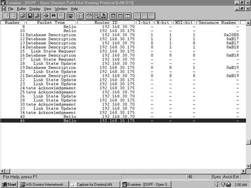
In Example 8-7, the output of the command debug ip ospf adj shows the adjacency of Figure 8-8 being built from the perspective of one of the routers (router ID 192.168.30.175).
Example 8-7. This debug output shows the adjacency events of Figure 8-8 from the perspective of one of the routers.
Degas#debug ip ospf adj
OSPF adjacency events debugging is on
OSPF: Rcv DBD from 192.168.30.70 on Ethernet0 seq 0x20E0 opt 0x2 flag 0x7 len 32
state INIT
OSPF: 2 Way Communication to 192.168.30.70 on Ethernet0,
  state 2WAY
OSPF: Neighbor change Event on interface Ethernet0
OSPF: DR/BDR election on Ethernet0
OSPF: Elect BDR 192.168.30.70
OSPF: Elect DR 192.168.30.175
   DR: 192.168.30.175 (Id) BDR: 192.168.30.70 (Id)
OSPF: Send DBD to 192.168.30.70 on Ethernet0 seq 0xB17 opt 0x2 flag 0x7 len 32
OSPF: First DBD and we are not SLAVE
OSPF: Rcv DBD from 192.168.30.70 on Ethernet0 seq 0xB17 opt 0x2 flag 0x2 len 92
state EXSTART
OSPF: NBR Negotiation Done. We are the MASTER
OSPF: Send DBD to 192.168.30.70 on Ethernet0 seq 0xB18 opt 0x2 flag 0x3 len 72
OSPF: Database request to 192.168.30.70
OSPF: Rcv DBD from 192.168.30.70 on Ethernet0 seq 0xB18 opt 0x2 flag 0x0 len 32
state EXCHANGE
OSPF: Send DBD to 192.168.30.70 on Ethernet0 seq 0xB19 opt 0x2 flag 0x1 len 32
OSPF: Rcv DBD from 192.168.30.70 on Ethernet0 seq 0xB19 opt 0x2 flag 0x0 len 32
state EXCHANGE
OSPF: Exchange Done with 192.168.30.70 on Ethernet0
OSPF: Synchronized with 192.168.30.70 on Ethernet0,
state FULL
At the end of the synchronization process in Figure 8-8, a series of Link State Update and Link State Acknowledgment packets can be observed. These are part of the LSA flooding process, discussed in the next section.
The entire OSPF topology can be depicted as a group of routers, or nodes, interconnected not by physical links but by logical adjacencies (Figure 8-9). For the nodes to route properly over this logical topology, each node must possess an identical map of the topology. This map is the topological database.

Figure 8-9. A group of routers interconnected by data links will be viewed by OSPF as a group of nodes interconnected by adjacencies.
The OSPF topological database is better known as the link-state database. This database consists of all the LSAs the router has received. A change in the topology is represented as a change in one or more of the LSAs. Flooding is the process by which these changed or new LSAs are sent throughout the network, to ensure that the database of every node is updated and remains identical to all other nodes’ databases.
Flooding makes use of the following two OSPF packet types:
Link State Update packets (type 4)
Link State Acknowledgment packets (type 5)
As Figure 8-10 shows, each Link State Update and Acknowledgment packet may carry multiple LSAs. Although the LSAs themselves are flooded throughout the area, the Update and Acknowledgment packets travel only between two nodes across an adjacency.
On point-to-point networks, updates are sent to the multicast address AllSPFRouters (224.0.0.5). On point-to-multipoint and virtual link networks, updates are unicasted to the interface addresses of the adjacent neighbors.
On broadcast networks, DRothers form adjacencies only with the DR and BDR. Therefore, updates are sent to the address AllDRouters (224.0.0.6). The DR in turn multicasts an Update packet containing the LSA to all adjacent routers on the network using the address AllSPFRouters. All routers then flood the LSA out all other interfaces (Figure 8-11). Although the BDR hears and records LSAs multicast from DRothers, it does not reflood or acknowledge them unless the DR fails to do so. The same DR/BDR functionality exists on NBMA networks, except that LSAs are unicast from DRothers to the DR and BDR, and the DR unicasts a copy of the LSA to all adjacent neighbors.

Figure 8-11. On a broadcast network, a DRother sends an LSA only to the DR and BDR (a); the DR refloods the LSA to all adjacent neighbors (b); all routers then flood the LSA on all other interfaces (c).
Because identical link-state databases are essential to correct OSPF operation, flooding must be reliable. Transmitting routers must know that their LSAs were received successfully, and receiving routers must know that they are accepting the correct LSAs.
Each individual transmitted LSA must be acknowledged. This may be accomplished by either an implicit acknowledgment or an explicit acknowledgment.
A neighbor can implicitly acknowledge the receipt of an LSA by including a duplicate of the LSA in an update back to the originator. Implicit acknowledgments are more efficient than explicit acknowledgments in some situations, such as when the neighbor was intending to send an update to the originator anyway.
A neighbor explicitly acknowledges the receipt of an LSA by sending a Link State Acknowledgment packet. A single Link State Acknowledgment packet is capable of acknowledging multiple LSAs. The packet carries only LSA headers—enough to completely identify the LSA—not the complete LSA.
When a router first sends an LSA, a copy of the LSA is entered into the Link State Retransmission list of every neighbor to which it was sent. The LSA is retransmitted every RxmtInterval until it is acknowledged or until the adjacency is broken. The Link State Update packets containing retransmissions are always unicast, regardless of the network type.
Acknowledgments might be either delayed or direct. By delaying an acknowledgment, more LSAs can be acknowledged in a single Link State Acknowledgment packet; on a broadcast network, LSAs from multiple neighbors can be acknowledged in a single multicast Link State Acknowledgment packet. The period by which an acknowledgment is delayed must be less than the RxmtInterval to prevent unnecessary retransmissions. Under normal circumstances, the unicast/multicast addressing conventions used for Link State Update packets on various network types also apply to Link State Acknowledgments.
Direct acknowledgments are always sent immediately and are always unicast. Direct acknowledgments are sent whenever the following conditions occur:
A duplicate LSA is received from a neighbor, possibly indicating that it has not yet received an acknowledgment.
The LSA’s age is MaxAge (described in the next section), and there is no instance of the LSA in the receiving router’s link-state database.
Each LSA contains three values that are used to ensure that the most recent copy of the LSA exists in every database. These values are sequence number, checksum, and age.
OSPF uses a 32-bit signed, linear sequence number space (discussed in Chapter 4, “Dynamic Routing Protocols”) ranging from InitialSequenceNumber (0x80000001) to MaxSequenceNumber (0x7fffffff). When a router originates an LSA, the router sets the LSA’s sequence number to InitialSequenceNumber. Each time the router produces a new instance of the LSA, the router increments the sequence number by one.
If the present sequence number is MaxSequenceNumber and a new instance of the LSA must be created, the router must first flush the old LSA from all databases. This is done by setting the age of the existing LSA to MaxAge (defined later in this section) and reflooding it over all adjacencies. As soon as all adjacent neighbors have acknowledged the prematurely aged LSA, the new instance of the LSA with a sequence number of InitialSequenceNumber may be flooded.
The checksum is a 16-bit integer calculated using a Fletcher algorithm.[12] The checksum is calculated over the entire LSA with the exception of the Age field (which changes as the LSA passes from node to node and would therefore require recalculation of the checksum at each node). The checksum of each LSA is also verified every five minutes as it resides in the link-state database, to ensure that it has not been corrupted in the database.
The age is an unsigned 16-bit integer that indicates the age of the LSA in seconds. The range is 0 to 3600 (one hour, known as MaxAge). When a router originates an LSA, the router sets the age to 0. As the flooded LSA transits a router, the age is incremented by a number of seconds specified by InfTransDelay. Cisco routers have a default InfTransDelay of one second, which can be changed with the command ip ospf transmit-delay. The age is also incremented as it resides in the database.
When an LSA reaches MaxAge, the LSA is reflooded and then flushed from the database. When a router needs to flush an LSA from all databases, it prematurely sets the age to MaxAge and refloods it. Only the router that originated the LSA can prematurely age it.
Example 8-8 shows a portion of a link-state database; the age, sequence number, and checksum of each LSA can be observed. More detailed discussion of the database and the various LSA types is in “Link-State Database,” later in this chapter.
Example 8-8. The age, sequence number, and checksum for each LSA are recorded in the link-state database. The age is incremented in seconds.
Manet#show ip ospf database
       OSPF Router with ID (192.168.30.43) (Process ID 1)
                   Router Link States (Area 3)
Link ID        ADV Router     Age   Seq#        Checksum Link Count
192.168.30.13  192.168.30.13  910   0x80000F29  0xA94E   2
192.168.30.23  192.168.30.23  1334  0x80000F55  0x8D53   3
192.168.30.30  192.168.30.30  327   0x800011CA  0x523    8
192.168.30.33  192.168.30.33  70    0x80000AF4  0x94DD   3
192.168.30.43  192.168.30.43  1697  0x80000F2F  0x1DA1   2
When multiple instances of the same LSA are received, a router determines which is the most recent by the following algorithm:
Compare the sequence numbers. The LSA with the highest sequence number is more recent.
If the sequence numbers are equal, then compare the checksums. The LSA with the highest unsigned checksum is the more recent.
If the checksums are equal, then compare the age. If only one of the LSAs has an age of MaxAge (3600 seconds), it is considered the more recent.
If the ages of the LSAs differ by more than 15 minutes (known as MaxAgeDiff), the LSA with the lower age is more recent.
If none of the preceding conditions are met, the two LSAs are considered identical.
The reader should by now have a good feel for why OSPF, with its multiple databases and complex algorithms, can put greater demands on the memory and processors of a router than the previously examined protocols can. As a network grows, these demands can become significant or even crippling. And although flooding is more efficient than the periodic, full-table updates of RIP, it can still place an unacceptable burden on the data links of a large network. Contrary to popular belief, the SPF algorithm itself is not particularly processor-intensive. Rather, the related processes, such as flooding and database maintenance, burden the CPU.
OSPF uses areas to reduce these adverse effects. In the context of OSPF, an area is a logical grouping of OSPF routers and links that effectively divide an OSPF domain into sub-domains (Figure 8-12). Routers within an area will have no detailed knowledge of the topology outside of their area. Because of this condition
A router must share an identical link-state database only with the other routers in its area, not with the entire OSPF domain. The reduced size of the database reduces the impact on a router’s memory.
The smaller link-state databases mean fewer LSAs to process and therefore less impact on the CPU.
Because the link-state database must be maintained only within an area, most flooding is also limited to the area.

Figure 8-12. An OSPF area is a logical grouping of OSPF routers. Each area is described by its own link-state database, and each router must maintain a database only for the area to which it belongs.
Areas are identified by a 32-bit Area ID. As Figure 8-12 shows, the Area ID may be expressed either as a decimal number or in dotted decimal, and the two formats may be used together on Cisco routers. The choice usually depends on which format is more convenient for identifying the particular Area ID. For example, area 0 and area 0.0.0.0 are equivalent, as are area 16 and area 0.0.0.16, and area 271 and area 0.0.1.15. In each of these cases, the decimal format would probably be preferred. However, given the choice of area 3232243229 and area 192.168.30.29, the latter would probably be chosen.
Three types of traffic may be defined in relation to areas:
Intra-area traffic consists of packets that are passed between routers within a single area.
Inter-area traffic consists of packets that are passed between routers in different areas.
External traffic consists of packets that are passed between a router within the OSPF domain and a router within another routing domain.
Area ID 0 (or 0.0.0.0) is reserved for the backbone. The backbone is responsible for summarizing the topologies of each area to every other area. For this reason, all inter-area traffic must pass through the backbone; non-backbone areas cannot exchange packets directly.
Many OSPF designers have a favorite rule of thumb concerning the maximum number of routers that an area can handle. This number might range from 30 to 200. However, the number of routers has little actual bearing on the maximum size of an area. Far more important factors include the number of links in an area, the stability of the topology, the memory and horsepower of the routers, the use of summarization, and the number of summary LSAs entering the area. Because of these factors, 25 routers might be too many for some areas, and other areas might accommodate well over 500 routers.
It is perfectly reasonable to design a small OSPF network with only a single area. Regardless of number of areas, a potential problem arises when an area is so underpopulated that no redundant links exist within it. If such an area becomes partitioned, service disruptions might occur. Partitioned areas are discussed in more detail in a later section.
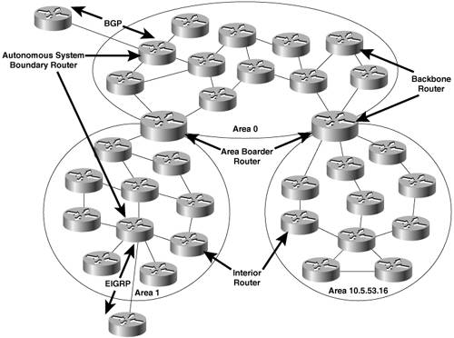
Routers, like traffic, can be categorized in relation to areas. All OSPF routers will be one of four router types, as shown in Figure 8-13:
Internal Routers are routers whose interfaces all belong to the same area. These routers have a single link-state database.
Area Border Routers (ABRs) connect one or more areas to the backbone and act as a gateway for inter-area traffic. An ABR always has at least one interface that belongs to the backbone, and must maintain a separate link-state database for each of its connected areas. For this reason, ABRs often have more memory and perhaps more powerful processors than internal routers. An ABR summarizes the topological information of its attached areas into the backbone, which then propagates the summary information to the other areas.
Backbone Routers are routers with at least one interface attached to the backbone. Although this requirement means that ABRs are also Backbone Routers, Figure 8-13 shows that not all Backbone Routers are ABRs. An Internal Router whose interfaces all belong to area 0 is also a Backbone Router.
Autonomous System Boundary Routers (ASBRs) are gateways for external traffic, injecting routes into the OSPF domain that were learned (redistributed) from some other protocol, such as the BGP and EIGRP processes shown in Figure 8-13. An ASBR can be located anywhere within the OSPF autonomous system except within stub areas; it may be an Internal, Backbone, or ABR.
A partitioned area is an area in which a link failure causes one part of the area to become isolated from another. If a non-backbone area becomes partitioned and if all routers on either side of the partition can still find an ABR, as in Figure 8-14, no service disruptions will occur. The backbone merely treats the partitioned area as two separate areas. Intra-area traffic from one side of the partition to the other side will become inter-area traffic, passing through the backbone to circumvent the partition. Note that a partitioned area is not the same as an isolated area, in which no path exists to the rest of the OSPF domain.
Figure 8-14. (a) Area 3 is connected to the backbone (area 0) by two ABRs. (b) A link failure in area 3 creates a partitioned area, but all routers within area 3 can still reach an ABR. In these circumstances, traffic can still be routed between the two sides of the partitioned area.
A partition of the backbone itself is a more serious matter. As Figure 8-15 shows, a partitioned backbone area isolates the areas on each side of the partition, creating two separate OSPF domains.

Figure 8-15. If a backbone becomes partitioned, each side of the partition and any connected areas become isolated from the other side.
Figure 8-16 shows some better area designs. Both area 0 and area 2 are designed so that neither of them can be partitioned by a single link failure. The vulnerability of area 2, however, is that if the ABR fails, the area will be isolated. Area 3 uses two ABRs; here, neither a single link failure nor a single ABR failure can isolate any part of the area.
A virtual link is a link to the backbone through a non-backbone area. Virtual links are used for the following purposes:
To link an area to the backbone through a non-backbone area (Figure 8-17)
To connect the two parts of a partitioned backbone through a nonbackbone area (Figure 8-18)


In both examples, the virtual link is not associated with a particular physical link. The virtual link is a tunnel through which packets may be routed on the optimal path from one endpoint to the other.
Several rules are associated with the configuration of virtual links:
Virtual links must be configured between two ABRs.
The area through which the virtual link is configured, known as the transit area, must have full routing information.
The transit area cannot be a stub area.
As mentioned previously, OSPF classifies a virtual link as a network type. Specifically, the link is considered an unnumbered—that is, unaddressed—link, belonging to the backbone, between two ABRs. These ABRs are considered neighbors by virtue of the virtual link between them, although they are not linked physically. Within each ABR, the virtual link will transition to the fully functional point-to-point interface state when a route to the neighboring ABR is found in the route table. The cost of the link is the cost of the route to the neighbor. When the interface state becomes point-to-point, an adjacency is established across the virtual link.
Virtual links add a layer of complexity and troubleshooting difficulty to any network. It is best to avoid the need for them by ensuring that areas, particularly backbone areas, are designed with redundant links to prevent partitioning. When two or more networks are merged, sufficient planning should take place beforehand so that no area is left without a direct link to the backbone.
If a virtual link is configured, it should be used only as a temporary fix to an unavoidable topology problem. A virtual link is a flag marking a part of the network that needs to be reengineered. Permanent virtual links are virtually always a sign of a poorly designed network.
All valid LSAs received by a router are stored in its link-state database. The collected LSAs will describe a graph of the area topology. Because each router in an area calculates its shortest path tree from this database, it is imperative for accurate routing that all area databases are identical.
A list of the LSAs in a link-state database can be observed with the command show ip ospf database, as shown in Example 8-9. This list does not show all of the information stored for each LSA, but shows only the information in the LSA header. Note that this database contains LSAs from multiple areas, indicating that the router is an ABR.
Example 8-9. The command show ip ospf database displays a list of all LSAs in the link-state database.
Homer#show ip ospf database

OSPF Router with ID (192.168.30.50) (Process ID 1)

                   Router Link States (Area 0)

Link ID            ADV Router      Age   Seq#        Checksum   Link count
192.168.30.10      192.168.30.10   1010  0x80001416  0xA818     3
192.168.30.20      192.168.30.20   677   0x800013C9  0xDE18     3
192.168.30.70      192.168.30.70   857   0x80001448  0xFD79     3
192.168.30.80      192.168.30.80   1010  0x800014D1  0xEB5C     5

                   Net Link States (Area 0)

Link ID            ADV Router      Age   Seq#        Checksum
192.168.17.18     192.168.30.20    677   0x800001AD  0x849A
192.168.17.34     192.168.30.60    695   0x800003E2  0x4619
192.168.17.58     192.168.30.40    579   0x8000113C  0xF0D
192.168.17.73     192.168.30.70    857   0x8000044F  0xB0E7

                   Summary Net Link States (Area 0)

Link ID            ADV Router      Age   Seq#        Checksum
172.16.121.0       192.168.30.60   421   0x8000009F  0xD52
172.16.121.0       192.168.30.70   656   0x8000037F  0x86A
10.63.65.0         192.168.30.10   983   0x80000004  0x1EAA
10.63.65.0         192.168.30.80   962   0x80000004  0x780A

                   Summary ASB Link States (Area 0)

Link ID            ADV Router      Age   Seq#        Checksum
192.168.30.12      192.168.30.20   584   0x80000005  0xFC4C
192.168.30.12      192.168.30.30   56    0x80000004  0x45BA
172.20.57.254      192.168.30.70   664   0x800000CE  0xF2CF
172.20.57.254      192.168.30.80   963   0x80000295  0x23CC

                   Router Link States (Area 4)

Link ID            ADV Router      Age   Seq#         Checksum   Link count
192.168.30.14     192.168.30.14   311   0x80000EA5   0x93A0     7
192.168.30.24     192.168.30.24   685   0x80001333   0x6F56     6
192.168.30.50     192.168.30.50   116   0x80001056   0x42BF     2
192.168.30.54     192.168.30.54   1213  0x80000D1F   0x3385     2

                   Summary Net Link States (Area 4)

Link ID            ADV Router      Age   Seq#        Checksum
172.16.121.0       192.168.30.40   1231  0x80000D88  0x73BF
172.16.121.0       192.168.30.50   34    0x800003F4  0xF90D
10.63.65.0         192.168.30.40   1240  0x80000003  0x5110
10.63.65.0         192.168.30.50   42    0x80000005  0x1144

                   Summary ASB Link States (Area 4)

Link ID            ADV Router      Age   Seq#        Checksum
192.168.30.12      192.168.30.40   1240  0x80000006  0x6980
192.168.30.12      192.168.30.50   42    0x80000008  0xC423
172.20.57.254      192.168.30.40   1241  0x8000029B  0xEED8
172.20.57.254      192.168.30.50   43    0x800002A8  0x9818

                   AS External Link States

Link ID            ADV Router      Age   Seq#        Checksum   Tag
10.83.10.0         192.168.30.60   459   0x80000D49  0x9C0B     0
10.1.27.0          192.168.30.62   785   0x800000EB  0xB5CE     0
10.22.85.0         192.168.30.70   902   0x8000037D  0x1EC0     65502
10.22.85.0         192.168.30.80   1056  0x800001F7  0x6B4B     65502
Homer#
Most of the entries in Example 8-9 have been deleted for brevity; the actual link-state database contains 1,445 entries and four areas, as shown in Example 8-10.
Example 8-10. The command show ip ospf database database-summary displays the number of LSAs in a link-state database by area and by LSA type.
Homer#show ip ospf database database-summary

            OSPF Router with ID (192.168.30.50) (Process ID 1)

Area ID        Router  Network  Sum-Net  Sum-ASBR  Subtotal  Delete  Maxage
0              8       4        185      27        224       0       0
4              7       0        216      26        249       0       0
5              7       0        107      13        127       0       0
56             2       1        236      26        265       0       0
AS External                                        580       0       0
Total          24      5        744      92        1445
Homer#
As mentioned earlier in “Reliable Flooding: Sequencing, Checksums, and Aging,” the LSAs are aged as they reside in the link-state database. If they reach MaxAge (1 hour), they are flushed from the OSPF domain. The implication here is that there must be a mechanism for preventing legitimate LSAs from reaching MaxAge and being flushed. This mechanism is the link-state refresh. Every 30 minutes, known as the LSRefreshTime, the router that originated the LSA floods a new copy of the LSA with an incremented sequence number and an age of zero. Upon receipt, the other OSPF routers replace the old copy of the LSA and begin aging the new copy.
So the link-state refresh process can be thought of as a keepalive for each LSA. An additional benefit is that any LSAs that might have become corrupted in a router’s LS database are replaced with the refreshed copy of the legitimate LSA.
The idea behind associating an individual refresh timer with each LSA is that the LSRefreshTime of the LSAs do not expire all at once, reflooding all LSAs every 30 minutes. Instead, the reflooding is spread out in a semi-random pattern. The problem with this approach is that with each individual LSA being reflooded as its LSRefreshTime expires, bandwidth is used inefficiently. Update packets can be transmitted with only a few, or even a single, LSA.
Prior to IOS 11.3, Cisco chose to have a single LSRefreshTime associated with the entire LS database. Every 30 minutes, each router refreshes all of the LSAs it originated, regardless of their actual age. Although this strategy avoids the problem of inefficiency, it reintroduces the problem the individual refresh timers were meant to solve. If the LS database is large, each router can create spikes in the area traffic and CPU usage every half hour.
Therefore a mechanism known as LSA group pacing was introduced to reach a compromise between the problems of individual refresh timers and a single monolithic timer. Each LSA has its own refresh timer, but as the individual refresh timers expire, a delay is introduced before the LSAs are flooded. By delaying the refresh, more LSAs can be grouped together before being flooded, so that Update packets are carrying a larger number of LSAs. By default, the group-pacing interval is 240 seconds (4 minutes). Depending on the IOS version, the default can be changed with either timers lsa-group-pacing or timers pacing lsa-group.[13] If the database is very large (10,000 or more LSAs), decreasing the group pacing interval is beneficial; if the database is small, increasing the interval might be useful. The range of the group pacing timer is 10 to 1800 seconds.
Because of the multiple router types defined by OSPF, multiple types of LSA are also necessary. For example, a DR must advertise the multi-access link and all the routers attached to the link. Other router types would not advertise this type of information. Both Example 8-9 and Example 8-10 show that there are multiple types of LSAs. Each type describes a different aspect of an OSPF network. Table 8-4 lists the LSA types and the type codes that identify them.
Router LSAs are produced by every router (Figure 8-19). This most fundamental LSA lists all of a router’s links, or interfaces, the state and outgoing cost of each link, and any known OSPF neighbors on the link. These LSAs are flooded only within the area in which they are originated. The command show ip ospf database router will list all of the Router LSAs in a database. Example 8-11 shows a variant of the command, in which a single router LSA is observed by specifying the router’s ID. As this and the subsequent illustrations show, the complete LSA is recorded in the link-state database. For a description of all the LSA fields, see the “OSPF Packet Formats” section later in this chapter.
Example 8-11. The command show ip ospf database router displays Router LSAs from the link-state database.
Homer#show ip ospf database router 192.168.30.10

      OSPF Router with ID (192.168.30.50) (Process ID 1)

                    Router Link States (Area 0)

Routing Bit Set on this LSA
LS age: 680
Options: (No TOS-capability)
LS Type: Router Links
Link State ID: 192.168.30.10
Advertising Router: 192.168.30.10
LS Seq Number: 80001428
Checksum: 0x842A
Length: 60
Area Border Router
 Number of Links: 3

  Link connected to: another Router (point-to-point)
   (Link ID) Neighboring Router ID: 192.168.30.80
   (Link Data) Router Interface address: 192.168.17.9
    Number of TOS metrics: 0
     TOS 0 Metrics: 64

  Link connected to: a Stub Network
   (Link ID) Network/subnet number: 192.168.17.8
   (Link Data) Network Mask: 255.255.255.248
    Number of TOS metrics: 0
     TOS 0 Metrics: 64

  Link connected to: a Transit Network
   (Link ID) Designated Router address: 192.168.17.18
   (Link Data) Router Interface address: 192.168.17.17
    Number of TOS metrics: 0
     TOS 0 Metrics: 10

Homer#
One line you will notice in Example 8-11 and in several subsequent LSA displays is the statement “Routing Bit Set on this LSA.” The routing bit is not a part of the LSA itself; it is an internal maintenance bit used by IOS indicating that the route to the destination advertised by this LSA is valid. So when you see “Routing Bit Set on this LSA,” it means that the route to this destination is in the routing table.
Network LSAs are produced by the DR on every multi-access network (Figure 8-20). As discussed earlier, the DR represents the multi-access network and all attached routers as a pseudonode, or a single virtual router. In this sense, a Network LSA represents a pseudonode just as a Router LSA represents a single physical router. The Network LSA lists all attached routers, including the DR itself. Like Router LSAs, Network LSAs are flooded only within the originating area. In Example 8-12, the command show ip ospf database network is used to observe a Network LSA.

Figure 8-20. A DR originates a Network LSA to represent a multi-access network and all attached routers.
Example 8-12. Network LSAs can be observed with the command show ip ospf database network.
Homer#show ip ospf database network 192.168.17.18

       OSPF Router with ID (192.168.30.50) (Process ID 1)

                    Net Link States (Area 0)

Routing Bit Set on this LSA
LS age: 244
Options: (No TOS-capability)
LS Type: Network Links
Link State ID: 192.168.17.18 (address of Designated Router)
Advertising Router: 192.168.30.20
LS Seq Number: 800001BF
Checksum: 0x60AC
Length: 32
Network Mask: /29
      Attached Router: 192.168.30.20
      Attached Router: 192.168.30.10
      Attached Router: 192.168.30.30

Homer#
Notice that unlike the Router LSA, there is no metric field in the Network LSA. This is because, as explained earlier in this chapter, the cost from the pseudonode represented by the LSA to any attached router is always 0.
Network Summary LSAs are originated by ABRs. They are sent into a single area to advertise destinations outside that area (Figure 8-21). In effect, these LSAs are the means by which an ABR tells the internal routers of an attached area what destinations the ABR can reach. An ABR also advertises the destinations within its attached areas into the backbone with Network Summary LSAs. Default routes external to the area, but internal to the OSPF autonomous system, are also advertised by this LSA type. The command show ip ospf database summary is used to display the network summary LSAs in the database, as shown in Example 8-13.

Example 8-13. Network Summary LSAs can be observed with the command show ip ospf database summary.
Homer#show ip ospf database summary 172.16.121.0

       OSPF Router with ID (192.168.30.50) (Process ID 1)

                    Summary Net Link States (Area 0)

Routing Bit Set on this LSA
LS age: 214
Options: (No TOS-capability)
LS Type: Summary Links(Network)
Link State ID: 172.16.121.0 (summary Network Number)
Advertising Router: 192.168.30.60
LS Seq Number: 800000B1
Checksum: 0xE864
Length: 28
Network Mask: /24
   TOS: 0 Metric: 791
When an ABR originates a Network Summary LSA, it includes the cost from itself to the destination the LSA is advertising. The ABR will originate only a single Network Summary LSA for each destination even if it knows of multiple routes to the destination. Therefore, if an ABR knows of multiple routes to a destination within its own attached area, it originates a single Network Summary LSA into the backbone with the lowest cost of the multiple routes. Likewise, if an ABR receives multiple Network Summary LSAs from other ABRs across the backbone, the original ABR will choose the lowest cost advertised in the LSAs and advertise that one cost into its attached non-backbone areas.
When another router receives a Network Summary LSA from an ABR, it does not run the SPF algorithm. Rather, it simply adds the cost of the route to the ABR and the cost included in the LSA. A route to the advertised destination, via the ABR, is entered into the route table along with the calculated cost. This behavior—depending on an intermediate router instead of determining the full route to the destination—is distance vector behavior. So, while OSPF is a link-state protocol within an area, it uses a distance vector algorithm to find inter-area routes.[14]
ASBR Summary LSAs are also originated by ABRs. ASBR Summary LSAs are identical to Network Summary LSAs except that the destination they advertise is an ASBR (Figure 8-22), not a network. The command show ip ospf database asbr-summary is used to display ASBR Summary LSAs (Example 8-14). Note in the illustration that the destination is a host address, and the mask is zero; the destination advertised by an ASBR Summary LSA will always be a host address because it is a route to a router.
Example 8-14. ASBR Summary LSAs can be observed with the command show ip ospf database asbr-summary.
Homer#show ip ospf database asbr-summary

       OSPF Router with ID (192.168.30.50) (Process ID 1)

                    Summary ASB Link States (Area 0)

Routing Bit Set on this LSA
LS age: 1640
Options: (No TOS-capability)
LS Type: Summary Links (AS Boundary Router)
Link State ID: 192.168.30.12 (AS Boundary Router address)
Advertising Router: 192.168.30.20
LS Seq Number: 80000009
Checksum: 0xF450
Length: 28
Network Mask: /0
   TOS: 0 Metric: 64
--More-
Autonomous System External LSAs, or External LSAs, are originated by ASBRs. They advertise either a destination external to the OSPF autonomous system, or a default route[15] external to the OSPF autonomous system (Figure 8-23). Referring back to Example 8-9, you can see that the AS External LSAs are the only LSA types in the database that are not associated with a particular area; external LSAs are flooded throughout the autonomous system. The command show ip ospf database external displays AS External LSAs (Example 8-15).
Example 8-15. AS External LSAs can be observed with the command show ip ospf database external.
Homer#show ip ospf database external 10.83.10.0

       OSPF Router with ID (192.168.30.50) (Process ID 1)

                    AS External Link States

Routing Bit Set on this LSA
LS age: 1680
Options: (No TOS-capability)
LS Type: AS External Link
Link State ID: 10.83.10.0 (External Network Number)
Advertising Router: 192.168.30.60
LS Seq Number: 80000D5A
Checksum: 0x7A1C
Length: 36
Network Mask: /24
      Metric Type: 1 (Comparable directly to link state metric)
      TOS: 0
      Metric: 10
      Forward Address: 172.20.57.254
      External Route Tag: 0
Homer#
Group Membership LSAs are used in an enhancement of OSPF known as Multicast OSPF (MOSPF).[16] MOSPF routes packets from a single source to multiple destinations, or group members, which share a class D multicast address. Although Cisco supports other multicast routing protocols, MOSPF is not supported as of this writing. For this reason, neither MOSPF nor the Group Membership LSA is covered in this book.
NSSA External LSAs are originated by ASBRs within not-so-stubby areas (NSSAs). NSSAs are described in the following section. An NSSA External LSA is almost identical to an AS External LSA, as the section on OSPF packet formats shows. Unlike AS External LSAs, which are flooded throughout an OSPF autonomous system, NSSA External LSAs are flooded only within the not-so-stubby area in which it was originated. The command show ip ospf database nssa-external displays NSSA External LSAs (Example 8-16).
Example 8-16. NSSA External LSAs can be observed with the command show ip ospf database nssa-external.
Morisot#show ip ospf database nssa-external

         OSPF Router with ID (10.3.0.1) (Process ID 1)

                     Type-7 AS External Link States (Area 15)

LS age: 532
Options: (No TOS-capability, No Type 7/5 translation, DC)
LS Type: AS External Link
Link State ID: 10.0.0.0 (External Network Number)
Advertising Router: 10.3.0.1
LS Seq Number: 80000001
Checksum: 0x9493
Length: 36
Network Mask: /16
      Metric Type: 2 (Larger than any link state path)
      TOS: 0
      Metric: 100
      Forward Address: 10.3.0.1
      External Route Tag: 0

--More-
External Attributes LSAs were proposed as an alternative to running Internal BGP (iBGP), to transport BGP information across an OSPF domain. This LSA has never been deployed on a wide scale, and is not supported in IOS.
Opaque LSAs are a class of LSAs that consist of a standard LSA header followed by application-specific information.[17] The Information field can be used directly by OSPF or indirectly by other applications to distribute information throughout the OSPF domain. Opaque LSAs have been used to add various extensions to OSPF, such as traffic engineering parameters for Multiprotocol Label Switching (MPLS) networks.
An ASBR learning external destinations will advertise those destinations by flooding AS External LSAs throughout the OSPF autonomous system. In many cases, these External LSAs may make up a large percentage of the LSAs in the databases of every router. For example, Example 8-10 shows that 580 of the LSAs in that database—40 percent—are external LSAs.
In Figure 8-24, not every router needs to know about all the external destinations. The routers in area 2 must send a packet to an ABR to reach the ASBR, no matter what the external destination might be. For this reason, area 2 can be configured as a stub area.
A stub area is an area into which AS External LSAs are not flooded. And if type 5 LSAs are not known inside an area, type 4 LSAs are unnecessary; these LSAs are also blocked. ABRs at the edge of a stub area use Network Summary (type 3) LSAs to advertise a single default route (destination 0.0.0.0) into the area. Any destination that the internal routers cannot match to an intra- or inter-area route will match the default route. Because the default route is carried in type 3 LSAs, it will not be advertised outside of the area.
The performance of routers within a stub area can be improved, and memory conserved, by the reduced size of their databases. Of course, the improvement will be more marked in OSPF domains with a large number of type 5 LSAs. There are, however, four restrictions on stub areas:
As in any area, all routers in a stub area must have identical link-state databases. To ensure this condition, all stub routers will set a flag (the E-bit) in their Hello packets to zero; they will not accept any Hello from a router in which the E-bit is set to one. As a result, adjacencies will not be established with any router that is not configured as a stub router.
Virtual links cannot be configured within, nor transit, a stub area.
No router within a stub area can be an ASBR. This restriction is intuitively understandable because ASBRs produce type 5 LSAs, and type 5 LSAs cannot exist within a stub area.
A stub area might have more than one ABR, but because of the default route, the internal routers cannot determine which router is the optimal gateway to the ASBR.
If memory is saved by blocking the propagation of type 5 and type 4 LSAs into an area, wouldn’t more memory be saved by blocking type 3 LSAs? In addressing this question, Cisco carries the concept of stub areas to its logical conclusion with a scheme known as totally stubby areas.
Totally stubby areas use a default route to reach not only destinations external to the autonomous system but also all destinations external to the area. The ABR of a totally stubby area will block not only AS External LSAs but also all Summary LSAs—with the exception of a single type 3 LSA to advertise the default route.
In Figure 8-25, a router with a few stub networks must be attached to the OSPF domain via one of the area 2 routers. The router supports only RIP, so the area 2 router will run RIP and redistribute the networks into OSPF. Unfortunately, this configuration makes the area 2 router an ASBR, and therefore area 2 can no longer be a stub area.
Figure 8-25. Because a few external destinations must be redistributed into OSPF at one of the area 2 routers, all of area 2 is ineligible to be a stub area.
The RIP speaker does not need to learn routes from OSPF—a default route pointing to the area 2 router is all it needs. But all OSPF routers must know about the networks attached to the RIP router to route packets to them.
Not-so-stubby areas (NSSAs)[18] allow external routes to be advertised into the OSPF autonomous system while retaining the characteristics of a stub area to the rest of the autonomous system. To do this, the ASBR in an NSSA will originate type 7 LSAs to advertise the external destinations. These NSSA External LSAs are flooded throughout the NSSA but are blocked at the ABR.
The NSSA External LSA has a flag in its header known as the P-bit. The NSSA ASBR has the option of setting or clearing the P-bit. If the NSSA’s ABR receives a type 7 LSA with the P-bit set to one, it will translate the type 7 LSA into a type 5 LSA and flood it throughout the other areas (see Figure 8-26). If the P-bit is set to zero, no translation will take place and the destination in the type 7 LSA will not be advertised outside of the NSSA. This option allows you to design an NSSA in which the external destinations learned in that area are known only in that area.

Figure 8-26. An ASBR within an NSSA will originate NSSA External LSAs. If the P-bit of an NSSA External LSA is set, the ABR will translate the LSA into an AS External LSA.
NSSAs are supported in IOS 11.2 and later.
Table 8-5 summarizes which LSAs are allowed in which areas.
The Dijkstra algorithm is used to calculate the Shortest Path Tree from the LSAs in the link state database. Chapter 4 has a somewhat detailed discussion of the Dijkstra algorithm; for a full description of the OSPF calculation of the SPF tree, see section 16.1 of RFC 2328.
OSPF determines the shortest path based on an arbitrary metric called cost, which is assigned to each interface. The cost of a route is the sum of the costs of all the outgoing interfaces to a destination. RFC 2328 does not specify any values for cost. Cisco routers calculate a default OSPF cost as 108/BW, where BW is the configured bandwidth of the interface and 108 is the reference bandwidth. As discussed previously, the default reference bandwidth can be changed with the command auto-cost reference-bandwidth. Fractional costs are rounded down to the nearest whole number. Table 8-6 shows the default costs calculated by this formula for some typical interfaces.
The command ip ospf cost can be used to override the default automatic cost calculations and assign a fixed cost to an interface. For example, a large network with homogeneous backbone link speeds might assign link costs based on line of sight or wire/fiber distance. LSAs record cost in a 16-bit field, so the total cost of an interface can range from 1 to 65535.
Each route entry is classified according to a destination type. The destination type will be either network or router.
Network entries are the addresses of networks to which packets can be routed. These are the destinations that are entered into the route table (Example 8-17).
Example 8-17. The OSPF entries in the route table are network destination types.
Homer#show ip route
Codes: C - connected, S - static, I - IGRP, R - RIP, M - mobile, B - BGP
       D - EIGRP, EX - EIGRP external, O - OSPF, IA - OSPF inter area
       E1 - OSPF external type 1, E2 - OSPF external type 2, E - EGP
       i - IS-IS, L1 - IS-IS level-1, L2 - IS-IS level-2, * - candidate default
       U - per-user static route

Gateway of last resort is 192.168.32.2 to network 0.0.0.0

O E1 192.168.118.0/24 [110/94] via 192.168.17.74, 02:15:01, Ethernet0
O E1 10.0.0.0/8 [110/84] via 192.168.17.41, 02:15:01, Serial0.19
O E1 192.168.119.0/24 [110/94] via 192.168.17.74, 02:15:01, Ethernet0
O E2 172.19.0.0/16 [110/21] via 192.168.32.2, 02:15:01, Ethernet1
     172.21.0.0/16 is variably subnetted, 2 subnets, 2 masks
O E2   172.21.0.0/16 [110/801] via 192.168.21.6, 02:15:01, Serial1.724
O      172.21.121.0/24 [110/791] via 192.168.21.6, 04:18:30, Serial1.724
     172.16.0.0/16 is variably subnetted, 104 subnets, 7 masks
O      172.16.21.48/30 [110/844] via 192.168.21.10, 04:18:48, Serial1.725
O IA   172.16.30.61/32 [110/856] via 192.168.17.74, 02:15:19, Ethernet0
O IA   172.16.35.0/24 [110/865] via 192.168.17.74, 02:15:19, Ethernet0
C      172.16.32.0/24 is directly connected, Ethernet1
O      172.16.17.48/29 [110/74] via 192.168.17.74, 06:19:46, Ethernet0
O E1   172.16.46.0/24 [110/30] via 192.168.32.2, 02:15:19, Ethernet1
O      172.16.45.0/24 [110/20] via 192.168.32.2, 3d10h, Ethernet1
O IA   172.16.30.54/32 [110/1061] via 192.168.17.74, 02:15:21, Ethernet0
O      172.16.17.56/29 [110/84] via 192.168.17.74, 06:19:48, Ethernet0
O      172.16.54.0/24 [110/11] via 192.168.32.2, 3d10h, Ethernet1
O      172.16.55.0/24 [110/11] via 192.168.32.2, 3d10h, Ethernet1
O      172.16.52.0/24 [110/11] via 192.168.32.2, 3d10h, Ethernet1
O      172.16.53.0/24 [110/11] via 192.168.32.2, 3d10h, Ethernet1
C      172.16.25.28/30 is directly connected, Tunnel29
--More-
Router entries are routes to ABRs and ASBRs. If a router needs to send a packet to an inter-area destination, it must know how to find an ABR; if a packet must go to an external destination, the router must know how to find an ASBR. Router entries contain this information, and are kept in a separate, internal route table. This table can be observed with the command show ip ospf border-routers (Example 8-18).
Example 8-18. Router entries, kept in a separate table from network entries, are routes to ABRs and ASBRs.
Homer#show ip ospf border-routers

OSPF Process 1 internal Routing Table

Codes: i - Intra-area route, I - Inter-area route
i 192.168.30.10 [74] via 192.168.17.74, Ethernet0, ABR, Area 0, SPF 391
I 192.168.30.12 [148] via 192.168.17.74, Ethernet0, ASBR, Area 0, SPF 391
I 192.168.30.18 [205] via 192.168.17.74, Ethernet0, ASBR, Area 0, SPF 391
i 192.168.30.20 [84] via 192.168.17.74, Ethernet0, ABR, Area 0, SPF 391
i 192.168.30.27 [781] via 192.168.21.6, Serial1.724, ASBR, Area 7, SPF 631
i 192.168.30.30 [74] via 192.168.17.74, Ethernet0, ABR/ASBR, Area 0, SPF 391
I 192.168.30.38 [269] via 192.168.17.74, Ethernet0, ASBR, Area 0, SPF 391
i 192.168.30.37 [390] via 192.168.21.10, Serial1.725, ASBR, Area 7, SPF 631
i 192.168.30.40 [84] via 192.168.17.74, Ethernet0, ABR/ASBR, Area 0, SPF 391
i 192.168.30.47 [400] via 192.168.21.10, Serial1.725, ASBR, Area 7, SPF 631
i 192.168.30.50 [74] via 192.168.17.41, Serial0.19, ABR/ASBR, Area 0, SPF 391
I 192.168.30.62 [94] via 192.168.17.74, Ethernet0, ASBR, Area 0, SPF 391
i 192.168.30.60 [64] via 192.168.17.41, Serial0.19, ABR/ASBR, Area 0, SPF 391
i 192.168.30.60 [790] via 192.168.21.10, Serial1.725, ABR/ASBR, Area 7, SPF 631
i 192.168.30.80 [10] via 192.168.32.5, Ethernet1, ABR/ASBR, Area 78, SPF 158
i 192.168.30.80 [10] via 192.168.17.74, Ethernet0, ABR/ASBR, Area 0, SPF 391
i 172.20.57.254 [10] via 192.168.32.2, Ethernet1, ASBR, Area 78, SPF 158
Homer#
As Example 8-18 shows, the internal route table looks very similar to any other route table—there are destinations, metrics, next-hop addresses, and exit interfaces. The difference is that all destinations are the Router IDs of ABRs and ASBRs. Each entry is tagged as intra-area (i) or inter-area (I), and the entry indicates whether the destination is an ABR, an ASBR, or both. The area is recorded, as is the iteration of the SPF algorithm that installed the entry.
Each route to a network destination is also classified as one of four path types. These path types are intra-area, inter-area, type 1 external, and type 2 external:
Intra-area paths are to destinations within one of the router’s attached areas.
Inter-area paths are to destinations in another area but within the OSPF autonomous system. An inter-area path, tagged with an IA in Example 8-17, always passes through at least one ABR.
Type 1 external paths (E1 in Example 8-17) are to destinations outside the OSPF autonomous system.
When an external route is redistributed into any autonomous system, it must be assigned a metric that is meaningful to the routing protocol of the autonomous system. Within OSPF, the ASBR is responsible for assigning a cost to the external routes they advertise. Type 1 external paths have a cost that is the sum of this external cost plus the cost of the path to the ASBR. Configuring an ASBR to advertise an external (redistributed) route with an E1 metric is covered in Chapter 11, “Route Redistribution.”
Type 2 external paths (E2) are also to destinations outside the OSPF autonomous system, but do not take into account the cost of the path to the ASBR.
E1 and E2 routes provide the network administrator with the option of choosing whether the internal cost to the ASBR is important or whether only the external cost of an external route, disregarding the internal cost of reaching the ASBR, is more important. For example, “hot potato” routing—getting packets to external destinations out of the network at the closest exit point—usually requires E1 metrics, whereas if you want packets to exit your network at the closest point to their external destination, use E2 metrics. OSPF external routes are, by default, E2 paths.
In Figure 8-27, router A has two paths to external destination 10.1.2.0. If the destination is advertised as E1, the A-B-D path will have a cost of 35 (5 + 20 + 10) and will be preferred over the A-C-D path whose cost is 50 (30 + 10 + 10). If the destination is advertised as E2, the cost of the two internal links to the ASBRs will be disregarded. In this case, the A-B-D path has a cost of 30 (20 + 10) and the A-C-D path has a cost of 20 (10 + 10). The latter will be the preferred path.
When an OSPF router examines the destination address of a packet, it takes the following steps to select the best route:[19]
Select the route or routes with the most specific match to the destination address. For example, if there are route entries for 172.16.64.0/18, 172.16.64.0/24, and 172.16.64.192/27, and the destination address is 172.16.64.205, the last entry will be chosen. The most specific match should always be the longest match—the route with the longest address mask. The entries may be host, subnet, network, supernet, or default addresses. If no match can be found, an ICMP Destination Unreachable message will be sent to the source address and the packet will be dropped.
Prune the set of selected entries by eliminating less-preferred path types. Path types are prioritized in the following order, with 1 being the most preferred and 4 being the least preferred:
1. Intra-area paths
2. Inter-area paths
3. E1 external paths
4. E2 external paths
If multiple equal-cost, equal-path-type routes exist in the final set, OSPF utilizes them. By default, the Cisco OSPF implementation load balances over a maximum of 16 equal-cost paths (four in older versions of IOS); this number can be changed within the range of one to six with the command maximum-paths.[20]
OSPF has the capability of authenticating all packets exchanged between neighbors. Authentication may be by simple passwords or by MD5 cryptographic checksums. These authentication methods are discussed in Chapter 6, “RIPv2, RIPng, and Classless Routing,” and examples of configuring OSPF authentication are given in the configuration section.
OSPF sends Hellos every 10 seconds and refreshes its LSAs every 30 minutes. These functions maintain the neighbor relationships, ensure that the link-state databases are accurate, and use less bandwidth than traditional distance vector protocols such as RIP. However, even this minimal traffic is undesirable on demand circuits—usage-sensitive connections such as X.25 SVCs, ISDN, and dialup lines. The recurring charges for such links may be determined by connect time or traffic volume or both, thus motivating the network manager to minimize their uptime.
An enhancement that makes OSPF practical over demand circuits is the capability of suppressing the Hello and LSA refresh functions so that a link does not have to be constantly up.[21] Although this enhancement is designed specifically for usage-sensitive circuits, it might be useful on any bandwidth-limited link.[22]
OSPF over demand circuits brings up a demand link to perform the initial database synchronization and subsequently brings up the link to flood only LSAs in which certain changes have occurred. These LSA changes are
A change in the LSA Options field.
A new instance of an existing LSA is received in which the age is MaxAge.
A change in the Length field of the LSA header.
A change in the contents of the LSA, excluding the 20-octet header, the checksum, or the sequence number.
Because no periodic Hellos are exchanged (Hellos are used only to bring up the link), OSPF must make a presumption of reachability. That is, it must presume that the demand circuit will be available when needed. In some instances, however, the link might not be immediately accessible. For example, a dialup link might be in use, both B channels of a BRI link might be in use, or the maximum number of allowed X.25 SVCs may already be up. In these situations, where the link is unavailable not because it is down but because of normal operational characteristics, the link is oversubscribed.
OSPF will not report an oversubscribed demand link as down, and packets routed to an oversubscribed link will be dropped rather than being queued. This behavior makes sense because there is no way to predict when the link will again become available; a stream of packets to an unavailable interface could overflow the buffers.
Several changes to the interface and neighbor state machines and to the flooding procedure must be made to support OSPF over demand circuits (see RFC 1793 for more details). Within the LSA format, two changes are made.
First, if LSAs are not periodically refreshed across a demand circuit, no routers on the other side of the link should declare the LSA invalid after MaxAge. The semantics of the LSA’s Age field are changed to accomplish this by designating the high bit as the DoNotAge bit. When an LSA is flooded over a demand circuit, the transmitting router will set DoNotAge = 1. As the LSA is flooded to all routers on the other side of the link, the Age field will be incremented normally by InfTransDelay seconds.[23] However, after being installed in a database, an LSA will not be aged like the other LSAs.
The second change derives from the first change. Because all routers must be capable of correctly interpreting the DoNotAge bit, a new flag known as the Demand Circuit bit (DC-bit) is added to all LSAs. By setting this flag in all LSAs it originates, a router signals to the other routers that it is capable of supporting OSPF over demand circuits.
A peripheral benefit of the enhancements made by OSPF over Demand Circuits—namely, designating the high bit of the Age field as the DoNotAge bit—is that you can now reduce flooding in stable topologies. With the command ip ospf flood-reduction entered for an interface, the DoNotAge bit is set on LSAs advertised out the interface and the LSAs are not refreshed unless they change.
The OSPF packet consists of multiple encapsulations, and deconstructing one is like peeling an onion. As shown in Figure 8-28, the outside of the onion is the IP header. Encapsulated within the IP header is one of five OSPF packet types. Each packet type begins with an OSPF packet header, whose format is the same for all packet types. The OSPF packet data following the header varies according to the packet type. Each packet type has a number of type-specific fields, followed by more data. The data contained in a Hello packet is a list of neighbors. LS Request packets contain a series of fields describing the requested LSAs. LS Update packets contain a list of LSAs, as shown in Figure 8-28. These LSAs in turn have their own headers and type-specific data fields. Database Description and LS Acknowledgment packets contain a list of LSA headers.
Note that OSPF packets are exchanged only between neighbors on a network. They are never routed beyond the network on which they originate.
Figure 8-29 shows an analyzer capture of an IP header for a packet carrying OSPF data, indicated by the protocol number of 89. When OSPF packets are multicast, their TTL is set to 1, as can be seen here. Because an OSPF packet should never be routed past an immediate neighbor, setting the TTL to 1 helps to ensure that the packet never travels more than a single hop. Some routers run processes that prioritize packets according to the Precedence bits (Weighted Fair Queuing and Weighted Random Early Detection, for example). OSPF sets the Precedence bits to Internetwork Control (110b), as shown in Figure 8-29, so that these processes will give a high priority to OSPF packets.
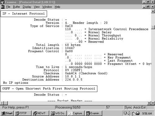
Figure 8-29. OSPF uses a protocol number of 89. It also sets the TTL value in the IP header to 1 and the Precedence bits to Internetwork Control.
This section details the five OSPF packet types, beginning with the header. The following section details the LSA types. An Options field is carried in Hello, Database Description packets, and in all LSAs. The format of this field is the same in all cases and is detailed in its own section.
All OSPF packets begin with a 24-octet header, as shown in Figure 8-30.

Version is the OSPF version number. The OSPF version number is 2. There is an OSPF version 3, created for routing IPv6; OSPFv3 is covered in the next chapter.
Type specifies the packet type following the header. Table 8-7 lists the five packet types by the number appearing in the Type field.
Packet length is the length of the OSPF packet, in octets, including the header.
Router ID is the ID of the originating router.
Area ID is the area from which the packet originated. If the packet is sent over a virtual link, the Area ID will be 0.0.0.0, the backbone Area ID, because virtual links are considered part of the backbone.
Checksum is a standard IP checksum of the entire packet, including the header.
AuType is the authentication mode being used.
Table 8-8 lists the possible authentication modes.
Authentication is the information necessary for the packet to be authenticated by whatever mode is specified in the AuType field. If AuType = 0, the field is not examined and therefore may contain anything. If AuType = 1, the field contains a password of up to 64 bits. If AuType = 2, the Authentication field contains a Key ID, the Authentication Data Length, and a nondecreasing Cryptographic sequence number. The message digest is appended to the end of the OSPF packet, and is not considered part of the packet itself.
Key ID identifies the authentication algorithm and the secret key used to create the message digest.
Authentication Data Length specifies the length, in octets, of the message digest appended to the end of the packet.
Cryptographic Sequence Number is a nondecreasing number used to prevent replay attacks.
The Hello packet (Figure 8-31) establishes and maintains adjacencies. The Hello carries parameters on which neighbors must agree in order to form an adjacency.

Network Mask is the address mask of the interface from which the packet was sent. If this mask does not match the mask of the interface on which the packet is received, the packet will be dropped. This technique ensures that routers become neighbors only if they agree on the exact address of their shared network.
Hello Interval, as discussed earlier, is the period, in seconds, between transmissions of Hello packets on the interface. If the sending and receiving routers don’t have the same value for this parameter, they do not establish a neighbor relationship.
Options are described in “Options Field,” later in this chapter. This field is included in the Hello packet to ensure that neighbors have compatible capabilities. A router might reject a neighbor because of a capabilities mismatch.
Router Priority is used in the election of the DR and BDR. If set to zero, the originating router is ineligible to become the DR or BDR.
Router Dead Interval is the number of seconds the originating router will wait for a Hello from a neighbor before declaring the neighbor dead. If a Hello is received in which this number does not match the RouterDeadInterval of the receiving interface, the packet is dropped. This technique ensures that neighbors agree on this parameter.
Designated Router is the IP address of the interface of the DR on the network (not its Router ID). During the DR election process, this may only be the originating router’s idea of the DR, not the finally elected DR. If there is no DR (because one has not been elected or because the network type does not require DRs), this field is set to 0.0.0.0.
Backup DR is the IP address of the interface of the BDR on the network. Again, during the DR election process, this may only be the originating router’s idea of the BDR. If there is no BDR, this field is set to 0.0.0.0.
Neighbor is a recurring field that lists all RIDs of all neighbors on the network from which the originating router has received a valid Hello in the past RouterDeadInterval.
The Database Description packet (Figure 8-32) is used when an adjacency is being established (see “Building an Adjacency,” earlier in this chapter). The primary purpose of the DD packet is to describe some or all of the LSAs in the originator’s database so that the receiver can determine whether it has a matching LSA in its own database. This is done by listing the headers of the LSAs; the LSA header contains enough information to identify not only a particular LSA but also the most recent instance of that LSA. Because multiple DD packets may be exchanged during the database description process, flags are included for managing the exchange via a master/slave polling relationship.

Interface MTU is the size, in octets, of the largest IP packet that can be sent out the originator’s interface without fragmentation. This field is set to 0x0000 when the packet is sent over virtual links.
Options are described in “Options Field,” later in this chapter. The field is included in the Database Description packet so that a router may choose not to forward certain LSAs to a neighbor that doesn’t support the necessary capabilities.
The first five bits of the next octet are unused and are always set to 00000b.
I-bit, or Initial bit, is set to 1 when the packet is the initial packet in series of DD packets. Subsequent DD packets have I-bit = 0.
M-bit, or More bit, is set to 1 to indicate that the packet is not the last in a series of DD packets. The last DD packet has M-bit = 0.
MS-bit, or Master/Slave bit, is set to 1 to indicate that the originator is the master (that is, is in control of the polling process) during a database synchronization. The slave has MS-bit = 0.
DD Sequence Number ensures that the full sequence of DD packets is received in the database synchronization process. The sequence number is set by the master to some unique value in the first DD packet, and the sequence is incremented in subsequent packets.
LSA Headers list some or all of the headers of the LSAs in the originator’s link-state database. See the section “Link State Header,” for a full description of the LSA header; the header contains enough information to uniquely identify the LSA and the particular instance of the LSA.
As Database Description packets are received during the database synchronization process, a router takes note of any listed LSAs that are not in its database or are more recent than its own LSA. These LSAs are recorded in the Link State Request list. The router then sends one or more Link State Request packets (Figure 8-33) asking the neighbor for its copy of the LSAs on the Link State Request list. Note that the packet uniquely identifies the LSA by Type, ID, and Advertising Router fields of its header, but it does not request a specific instance of the LSA (identified by the header’s sequence number, checksum, and age). Therefore, the request is for the most recent instance of the LSA, whether the requester is aware of that instance or not. This procedure protects against a situation in which the neighbor might acquire or originate a more recent copy of the LSA between the time it last described the LSA and the time a copy of it is requested.

Link State Type is the LS type number, which identifies the LSA as a Router LSA, Network LSA, and so on. Type numbers are listed in Table 8-4.
Link State ID is a type-dependent field of the LSA header. See the section “Link State Header” and the LSA-specific sections for a full description of how the various LSAs use this field.
Advertising Router is the Router ID of the router that originated the LSA.
The Link State Update packet, shown in Figure 8-34, is used in the flooding of LSAs and to send LSAs in response to Link State Requests. Recall that OSPF packets do not leave the network on which they were originated. Consequently, a Link State Update packet, carrying one or many LSAs, carries the LSAs only to the originating router’s connected neighbors. The receiving neighbor is responsible for re-encapsulating the appropriate LSAs in new LS Update packets for further flooding to its own neighbors.

Number of LSAs specifies the number of LSAs included in this packet.
LSAs are the full LSAs as described in OSPF LSA formats. Each update can carry multiple LSAs, up to the maximum packet size allowed on the link.
Link State Acknowledgment packets are used to make the flooding of LSAs reliable. Each LSA received by a router from a neighbor must be explicitly acknowledged in a Link State Acknowledgement packet. The LSA being acknowledged is identified by including its header in the LS ACK packet, and multiple LSAs can be acknowledged in a single packet. As Figure 8-35 shows, the LS ACK packet consists of nothing more than an OSPF packet header and a list of LSA headers.
This section details the fields of LSA types 1-5 and 7. The Group Membership LSA (type 6) is not discussed because MOSPF is not covered in this book. Similarly, LSA types 8 through 11 are not covered because they either are not in general deployment (type 8) or because they are used to support capabilities that are outside of the scope of this book.
The LSA header (Figure 8-36) begins all LSAs and is also used by itself in Database Description and Link State Acknowledgment packets. Three fields in the header uniquely identify every LSA: the Type, Link State ID, and Advertising Router. Additionally, three other fields uniquely identify the most recent instance of an LSA: the Age, Sequence Number, and Checksum.
Age is the time, in seconds, since the LSA was originated. As the LSA is flooded, the age is incremented by InfTransDelay seconds at each router interface it exits. The age is also incremented in seconds as it resides in a link-state database.
Options is described in the section “Options Field.” In the LSA header, the Options field specifies the optional capabilities supported by the portion of the OSPF domain described by the LSA.
Type is the LSA type. The type codes are shown in Table 8-4.
Link State ID identifies the portion of the OSPF domain being described by the LSA. The specific usage of this field varies according to the LSA type; the descriptions of each LSA include a description of how the LSA uses this field.
Advertising Router is the router ID of the router that originated the LSA.
Sequence Number is incremented each time a new instance of the LSA is originated, so that other routers can identify the most recent instance of the LSA.
Checksum is the Fletcher checksum of the complete contents of the LSA except for the Age field. If the Age field were included, the checksum would have to be recalculated every time the age was incremented.
Length is the number of octets of the LSA, including the header.
A Router LSA (Figure 8-37) is produced by every router. It lists a router’s links, or interfaces, along with the state and the outgoing cost of each link and any known neighbors on the link. These LSAs are flooded only within the area in which they are originated. The command show ip ospf database router (refer to Example 8-11) lists the Router LSAs in a database. Note that Router LSAs advertise host routes as stub networks; the Link ID field carries the host IP address, and the Link Data field carries the host address mask of 255.255.255.255.
Link State ID for Router LSAs is the originating router’s Router ID.
V, or Virtual Link Endpoint bit, is set to one when the originating router is an endpoint of one or more fully adjacent virtual links having the described area as the transit area.
E, or External bit, is set to one when the originating router is an ASBR.
B, or Border bit, is set to one when the originating router is an ABR.
Number of Links specifies the number of router links the LSA describes. The Router LSA must describe all of the originating router’s links, or interfaces, to the area in which the LSA is flooded.
Subsequent fields in the Router LSA describe each link and appear one or more times, corresponding to the number in the Number of Links field. This discussion covers the Link Type field first, although that field does not appear until after the Link Data field. Understanding link type first is important because the descriptions of the Link ID and Link Data fields vary according to the value of the Link Type field.
Link Type describes the general type of connection the link provides. Table 8-9 lists the possible values of the field and the associated connection types.
Link ID identifies the object to which the link connects. This is dependent on the link type, as shown in Table 8-10. Note that when the connected object is another router, the Link ID is the same as the Link State ID in the header of the neighboring router’s LSA. During the routing table calculation, this value is used to find the neighbor’s LSA in the link-state database.
Link Data also depends on the value of the Link Type field, as shown in Table 8-11.
Table 8-11. Link data values.
Link Type
Value of Link Data Field
1
IP address of the originating router’s interface to the network[*]
2
IP address of the originating router’s interface to the network
3
Network’s IP address or subnet mask
4
The MIB-II ifIndex value for the originating router’s interface
[*] If the point-to-point link is unnumbered, this field will instead carry the MIB-II ifIndex value of the interface.
Number of TOS specifies the number of Type of Service metrics listed for this link. Although TOS is no longer supported in RFC 2328, the TOS fields are still included for backward compatibility with earlier OSPF implementations. If no TOS metrics are associated with a link, this field is set to 0x00.
Metric is the cost of the link (interface).
The next two fields are associated with a link corresponding to the number (#) of TOS field. For example, if # of TOS = 3, there will be three 32-bit words containing three instances of these fields. If # of TOS = 0, there will be no instances of these fields.
Note that Cisco supports only TOS = 0.
TOS specifies the Type of Service to which the following metric refers.[24] Table 8-12 lists the TOS values (as specified in RFC 1349), the bit values of the corresponding TOS field in the IP header, and the corresponding value used in the OSPF TOS field.
TOS Metric is the metric associated with the specified TOS value.
Network LSAs (Figure 8-38) are originated by DRs. These LSAs advertise the multi-access network, and all routers (including the DR) attached to the network. Like Router LSAs, Network LSAs are flooded only within the originating area. The command show ip ospf database network (Example 8-12) is used to observe a Network LSA.

Link State ID for Network LSAs is the IP address of the DR’s interface to the network.
Network Mask specifies the address or subnet mask used on this network.
Attached Router lists the Router IDs of all routers on the multi-access network that are fully adjacent with the DR, and the Router ID of the DR itself. The number of instances of this field (and hence the number of routers listed) can be deduced from the LSA header’s Length field.
The Network Summary LSA (type 3) and the ASBR Summary LSA (type 4) have an identical format, shown in Figure 8-39. The only difference in field contents is the Type and the Link State ID. ABRs produce both types of Summary LSA; Network Summary LSAs advertise networks external to an area (including default routes), whereas ASBR Summary LSAs advertise ASBRs external to an area. Both types are flooded only into a single area. The Network Summary LSAs in a router’s database can be observed with the command show ip ospf database summary (Example 8-13), and ASBR Summary LSAs can be observed with show ip ospf database asbr-summary (Example 8-14).

Link State ID, for type 3 LSAs, is the IP address of the network or subnet being advertised. If the LSA is type 4, the Link State ID is the Router ID of the ASBR being advertised.
Network Mask is the address or subnet mask of the network being advertised in type 3 LSAs. In type 4 LSAs, this field has no meaning and is set to 0.0.0.0.
If a type 3 LSA is advertising a default route, both the Link State ID and the Network Mask fields will be 0.0.0.0.
Metric is the cost of the route to this destination.
The TOS and TOS Metric fields are optional and are described in “Router LSA.” Again, Cisco supports only TOS = 0.
Autonomous System External LSAs (Figure 8-40) are originated by ASBRs. These LSAs are used to advertise destinations external to the OSPF autonomous system, including default routes to external destinations, and are flooded into all nonstub areas of the OSPF domain. The command show ip ospf database external is used to display AS External LSAs (Example 8-15).

Link State ID for AS External LSAs is the IP address of the destination.
Network Mask is the address or subnet mask for the destination being advertised.
If the type 5 LSA is advertising a default route, the Link State ID and the Network Mask are both 0.0.0.0.
E, or External Metric bit, specifies the type of external metric to be used with this route. If the E-bit is set to 1, the metric type is E2. If the E-bit = 0, the metric type is E1. See the section “Path Types,” earlier in this chapter, for more information on E1 and E2 external metrics.
Metric is the cost of the route, as set by the ASBR.
Forwarding Address is the address to which packets for the advertised destination should be forwarded. If the forwarding address is 0.0.0.0, packets are forwarded to the originating ASBR.
External Route Tag is an arbitrary tag that may be applied to the external route. This field is not used by the OSPF protocol itself, but is instead provided for external route management. The setting and use of such tags are discussed in Chapter 14, “Route Maps.”
Optionally, TOS fields may be associated with the destination. These fields are the same as discussed previously, except each TOS metric also has its own E-bit, Forwarding Address, and External Route Tag.
NSSA External LSAs are originated by ASBRs within an NSSA (not-so-stubby area). All fields of the NSSA External LSA (Figure 8-41) are identical to an AS External LSA’s fields, with the exception of the Forwarding Address field. Unlike AS External LSAs, which are flooded throughout an OSPF autonomous system, NSSA external LSAs are flooded only within the not-so-stubby area in which it was originated. The command show ip ospf database nssa-external is used to display NSSA External LSAs (Example 8-16).
Forwarding Address, if the network between the NSSA ASBR and the adjacent autonomous system is advertised as an internal route, is the next hop address on the network. If the network is not advertised as an internal route, the forwarding address will be the NSSA ASBR’s Router ID.
The Options field (Figure 8-42) is present in every Hello and Database Description packet and in every LSA. The Options field allows routers to communicate their optional capabilities to other routers.
DN is used with MPLS-based layer 3 Virtual Private Networks (VPN), commonly called RFC 2547 VPNs after the RFC that specifies them. When a route is learned from a customer network via OSPF, is advertised across the RFC 2547 VPN using Multiprotocol BGP, and then is advertised back to a customer network via OSPF, a loop can occur in which the OSPF route is redistributed back to the VPN provider network in BGP. The DN bit prevents this looping. When the DN bit is set in a type 3, 5, or 7 LSA, the receiving router cannot use that LSA in its OSPF route calculations.
O is set to indicate that the originating router supports Opaque (type 9, 10, and 11) LSAs.
DC is set when the originating router is capable of supporting OSPF over demand circuits.
EA is set when the originating router is capable of receiving and forwarding External Attributes LSAs. These LSAs are not in general usage and are not covered in this book.
N is used only in Hello packets. A router sets N-bit = 1 to indicate support for NSSA External LSAs. If N-bit = 0, the router will not accept or send these LSAs. Neighboring routers with mismatched N-bits will not become adjacent; this restriction ensures that all routers in an area support NSSA capabilities equally. If the N-bit = 1, the E-bit must be 0.
P is used only in NSSA External LSA headers. (For this reason, the N- and P-bit can use the same position.) This bit tells the ABR of a not-so-stubby area to translate type 7 LSAs into type 5 LSAs.
MC is set when the originating router is capable of forwarding IP multicast packets. This bit is used by MOSPF.
E is set when the originating router is capable of accepting AS External LSAs. It will be set to 1 in all AS External LSAs and in all LSAs originated in the backbone and nonstub areas. E-bit = 0 in all LSAs originated within a stub area. Additionally, the bit is used in the Hello packet to indicate an interface’s capability of sending and receiving type 5 LSAs. Neighboring routers with mismatched E-bits will not become adjacent; this restriction ensures that all routers in an area support stub capabilities equally.
MT, when set, indicates that the originating router supports Multitopology OSPF (MT-OSPF). MT-OSPF, as of this writing, is only a proposal and has not yet found general adoption.
Older OSPF standards specified that the options bit position now occupied by the MT bit was the T bit. T was set when the originating router is capable of supporting TOS. However, because the TOS capability was never deployed, the T bit was also never used.
The many options and configuration variables available to OSPF frequently make it the IGP of choice in large IP networks. However, the opinion is occasionally expressed that OSPF configuration is “too complex” to be a good choice for small internets. This is nonsense. As the first case study shows, getting a basic OSPF configuration up and running involves only a few extra keystrokes in the network command; if the operation of OSPF is reasonably well understood, these extra keystrokes will be intuitive.
The three steps necessary to begin a basic OSPF process are
Determine the area to which each router interface will be attached.
Enable OSPF with the command router ospf process-id.
Specify the interfaces on which to run OSPF, and their areas, with the network area command.
Unlike the process ID associated with IGRP and EIGRP, the OSPF process ID is not an autonomous system number. The process ID can be any positive integer and has no significance outside the router on which it is configured. Cisco IOS allows multiple OSPF processes to run on the same router;[25] the process ID merely distinguishes one process from another within the device.
The network command used with RIP allows only the specification of a major network address. If some interfaces within the network should not run the routing protocol, the passive-interface command has to be used with those protocols. As is the network command used with the wildcard mask for EIGRP, the network area command is much more flexible then the network command used for RIP and EIGRP before the wildcard option was introduced, reflecting the fully classless nature of OSPF. Any address range can be specified with an (address, inverse mask) pair. The inverse mask is the same as the inverse mask used with access lists.[26] The area can be specified in either decimal or dotted decimal.
Figure 8-43 shows an OSPF network. Note that each area has an assigned IP address from which its subnets are derived. Limiting an area to a single address or subnet is not necessary, but doing so has significant advantages, as will be seen in a later case study on address summarization. Note also that this example is designed to demonstrate the configuration of multiple areas. In “real life,” it would be much wiser to put such a small network within a single area. Further, that single area does not have to be area 0. The rule is that all areas must connect to the backbone; therefore, a backbone area is needed only if there is more than one area.
Each of the four routers in Figure 8-43 is configured differently to demonstrate the flexibility of the network area command. The configurations are displayed in Example 8-19 through Example 8-22:
Example 8-19. Rubens’s OSPF network area configuration.
router ospf 10
 network 0.0.0.0 255.255.255.255 area 1
Example 8-20. Chardin’s OSPF network area configuration.
router ospf 20
 network 192.168.30.0 0.0.0.255 area 1
 network 192.168.20.0 0.0.0.255 area 0
Example 8-21. Goya’s OSPF network area configuration.
router ospf 30
 network 192.168.20.0 0.0.0.3 area 0.0.0.0
 network 192.168.10.0 0.0.0.31 area 192.168.10.0
Example 8-22. Matisse’s OSPF network area configuration.
router ospf 40
 network 192.168.10.2 0.0.0.0 area 192.168.10.0
 network 192.168.10.33 0.0.0.0 area 192.168.10.0
The first thing to note is that the process IDs are different for each router. Usually these numbers are the same across an internet for consistency of configuration. Here the process IDs are configured differently merely to demonstrate that they have no meaning outside of the router. These four differently numbered processes are able to communicate.
The next thing to notice is the format of the network area command. Following the network portion is an IP address and an inverse mask. When the OSPF process first becomes active, it will “run” the IP addresses of all active interfaces against the (address, inverse mask) pair of the first network statement. All interfaces that match will be assigned to the area specified by the area portion of the command. The process will then run the addresses of any interfaces that did not match the first network statement against the second network statement. The process of running IP addresses against network statements continues until all interfaces have been matched or until all network statements have been used. It is important to note that this process is consecutive, beginning with the first network statement. As a result, the order of the statements can be important, as is shown in the troubleshooting section.
Rubens’s network statement will match all interfaces on the router. The address 0.0.0.0 is really just a placeholder; the inverse mask of 255.255.255.255 is the element that does all of the work here. With “don’t care” bits placed across the entire four octets, the mask will find a match with any address and place the corresponding interface into area 1. This method provides the least precision in controlling which interfaces will run OSPF.
Chardin is an ABR between area 1 and area 0. This fact is reflected in its network statements. Here the (address, inverse mask) pairs will place any interface that is connected to any subnet of major network 192.168.30.0 in area 1 and any interface that is connected to any subnet of major network 192.168.20.0 in the backbone area.
Goya is also an ABR. Here the (address, inverse mask) pairs will match only the specific subnets configured on the two interfaces. Notice also that the backbone area is specified in dotted decimal. Both this format and the decimal format used at Chardin will cause the associated area fields of the OSPF packets to be 0x00000000, so they are compatible.
Matisse has one interface, 192.168.10.65/26, which is not running OSPF. The network statements for this router are configured to the individual interface addresses, and the inverse mask indicates that all 32 bits must match exactly. This method provides the most precise control over which interfaces will run OSPF.
Finally, note that although Matisse’s interface 192.168.10.65/26 is not running OSPF, that address is numerically the highest on the router. As a result, Matisse’s Router ID is 192.168.10.65 (Example 8-23).
Example 8-23. The command show ip ospf process-id displays process-specific information.
Matisse#show ip ospf 40
 Routing Process "ospf 40" with ID 192.168.10.65
 Supports only single TOS(TOS0) routes
 Supports opaque LSA
 Supports Link-local Signaling (LLS)
 Initial SPF schedule delay 5000 msecs
 Minimum hold time between two consecutive SPFs 10000 msecs
 Maximum wait time between two consecutive SPFs 10000 msecs
 Minimum LSA interval 5 secs. Minimum LSA arrival 1 secs
 LSA group pacing timer 240 secs
 Interface flood pacing timer 33 msecs
 Retransmission pacing timer 66 msecs
 Number of external LSA 0. Checksum Sum 0x000000
 Number of opaque AS LSA 0. Checksum Sum 0x000000
 Number of DCbitless external and opaque AS LSA 0
 Number of DoNotAge external and opaque AS LSA 0
 Number of areas in this router is 1. 1 normal 0 stub 0 nssa
 External flood list length 0
    Area 192.168.10.0
        Number of interfaces in this area is 2
        Area has no authentication
        SPF algorithm last executed 00:47:42.792 ago
        SPF algorithm executed 4 times
        Area ranges are
        Number of LSA 5. Checksum Sum 0x02A444
        Number of opaque link LSA 0. Checksum Sum 0x000000
        Number of DCbitless LSA 0
        Number of indication LSA 0
        Number of DoNotAge LSA 0
Flood list length 0Suppose router Matisse from Figure 8-43 has been configured in a staging center and then sent to the field to be installed. During the bootup, the router reports that it cannot allocate a Router ID, and it seems to report the network area commands as configuration errors (Example 8-24). Worse, the OSPF commands are no longer in the running configuration.
Example 8-24. OSPF will not boot if it cannot find an active IP address for its Router ID.
Cisco Internetwork Operating System Software
IOS (tm) C2600 Software (C2600-J1S3-M), Version 12.3(6), RELEASE SOFTWARE (fc3)
Copyright (c) 1986-2004 by Cisco Systems, Inc.
Compiled Wed 11-Feb-04 19:24 by kellythw
Image text-base: 0x80008098, data-base: 0x8199F778

cisco 2621 (MPC860) processor (revision 0x200) with 61440K/4096K bytes of memory


Processor board ID JAD05090PW2 (1141326406)
M860 processor: part number 0, mask 49
Bridging software.
X.25 software, Version 3.0.0.
TN3270 Emulation software.
2 FastEthernet/IEEE 802.3 interface(s)
1 Serial network interface(s)
32K bytes of non-volatile configuration memory.
16384K bytes of processor board System flash (Read/Write)


 network 192.168.10.2 0.0.0.0 area 192.168.10.0
    ^
% Invalid input detected at '^' marker.
 network 192.168.10.33 0.0.0.0 area 192.168.10.0
    ^
% Invalid input detected at '^' marker.


Press RETURN to get started!


%OSPF-4-NORTRID: OSPF process 40 cannot start. There must
be at least one "up" IP interface, for OSPF to use as router ID
The problem here is that during bootup all the interfaces on the router were administratively shut down. If OSPF cannot find an active IP address for its Router ID, it cannot start. And if the OSPF process isn’t active, the subsequent network area commands will be invalid.
The solution to this problem (assuming you have a valid reason for having all physical interfaces in shutdown) is to use a loopback interface. The loopback interface, which is a virtual, software-only interface, is always up. Therefore, its IP address is always available.
The more common reason for using loopback interfaces on OSPF routers is that the interfaces allow the network administrator to control the Router IDs. When the OSPF process looks for a Router ID, OSPF will prefer the address of a loopback interface over the addresses of all physical interfaces, regardless of the numerical order. If there are multiple loopback interfaces with IP addresses, OSPF will choose the numerically highest loopback address.
Controlling the Router IDs so that individual OSPF routers are more easily identified facilitates management and troubleshooting. The Router IDs are usually managed by one of two methods:
Set aside a legitimate network or subnet address to be used strictly for Router IDs.
Use a “bogus” IP address range.
The first method has the disadvantage of using up the assigned network address space. The second method will preserve the legitimate addresses, but one must remember that what is bogus in one internet is legitimate in another. Using easily recognized addresses such as 1.1.1.1, 2.2.1.1, and so on is fine as long as you remember that these are not public addresses. Care must be taken that the bogus addresses do not leak out to the public Internet.
The configurations of the last section are modified to use loopback addresses as displayed in Example 8-25 through Example 8-28.
Example 8-25. A Loopback interface is added to Rubens’s configuration.
interface Loopback0
 ip address 192.168.50.1 255.255.255.255
!
router ospf 10
 network 192.168.30.0 0.0.0.255 area 1
Example 8-26. A Loopback interface is added to Chardin’s configuration.
interface Loopback0
 ip address 192.168.50.2 255.255.255.255
!
router ospf 20
 network 192.168.30.0 0.0.0.255 area 1
 network 192.168.20.0 0.0.0.255 area 0
Example 8-27. A Loopback interface is added to Goya’s configuration.
interface Loopback0
 ip address 192.168.50.3 255.255.255.255
!
router ospf 30
 network 192.168.20.0 0.0.0.3 area 0.0.0.0
 network 192.168.10.0 0.0.0.31 area 192.168.10.0
Example 8-28. A Loopback interface is added to Matisse’s configuration.
interface Loopback0
 ip address 192.168.50.4 255.255.255.255
!
router ospf 40
 network 192.168.10.2 0.0.0.0 area 192.168.10.0
 network 192.168.10.33 0.0.0.0 area 192.168.10.0
For this example, the network address 192.168.50.0 has been set aside for exclusive use as Router IDs. Router IDs are thus easily distinguished from other IP addresses in this internet.
The first thing to note about this configuration is the address masks used with the loopback addresses: Each mask is configured as a host address. This step is not really necessary, because OSPF treats a loopback interface as a stub host; whatever (address, mask) pair is configured, the address of the loopback interface will be advertised as a host route. The host mask is used merely to keep things neat, and to reflect the way in which the address is advertised.
However, the second point of interest makes the first somewhat irrelevant. Remember that OSPF does not have to be running on an interface for its IP address to be used as the Router ID. In fact, having OSPF advertise the loopback addresses just creates unnecessary LSAs. In the example shown, notice that the network area statements do not refer to the loopback addresses. In fact, the configuration at Rubens had to be changed. Rubens’s previous command, network 0.0.0.0 255.255.255.255 area 1, would have picked up the loopback address.
In addition to aiding management and troubleshooting, using loopback interfaces will also make an OSPF internet more stable. In some early versions of IOS, if a physical interface from which the Router ID was taken experiences a hardware failure,[27] if the interface is administratively shut down, or if the IP address is inadvertently deleted, the OSPF process must acquire a new Router ID. Therefore, the router must prematurely age and flood its old LSAs and then flood LSAs containing the new ID. A loopback interface has no hardware components to fail. The current IOS behavior is to obtain the Router ID; if the interface associated with the Router ID fails or the IP address is deleted, the router retains the Router ID until the router is reloaded or the OSPF process is reset.
Another option is to manually assign a Router ID to the router with the OSPF command router-id. As with the Router ID address assignment using loopback interfaces, you can arbitrarily choose an IP address to use as the value of the router-id command. If a Router ID is configured using this command, this command’s value will become the router ID when the OSPF process is reset or the router is reloaded. When the router is reloaded, however, there still has to be an interface with an IP address that comes up before the OSPF process can start. After the OSPF process starts, the address assigned with the router-id command will become the Router ID.
Loopback interfaces simplify the management and troubleshooting of OSPF internets by providing predictable Router IDs. This simplification can be taken even further by recording the Router IDs in a Domain Name Service (DNS) database. The router can then be configured to consult the server address-to-name mappings, or Reverse DNS lookups, and then display the routers by name instead of by Router ID (Example 8-29).
Example 8-29. OSPF can be configured to use DNS to map Router IDs to names for use in some show commands.
Goya#show ip ospf neighbor

Neighbor ID     Pri   State      Dead Time    Address       Interface
chardin           0   FULL/  -   00:00:36     192.168.20.1  Serial0/0.2
matisse           0   FULL/  -   00:00:34     192.168.10.2  Serial0/0.1
Goya#show ip ospf database

            OSPF Router with ID (192.168.50.3) (Process ID 30)

                Router Link States (Area 0.0.0.0)

Link ID         ADV Router      Age         Seq#       Checksum Link count
192.168.50.2    chardin         78          0x80000007 0x005A70 2
192.168.50.3    goya            78          0x80000008 0x004C7B 2

                Summary Net Link States (Area 0.0.0.0)

Link ID         ADV Router      Age         Seq#       Checksum
192.168.10.0    goya            74          0x80000001 0x00B356
192.168.10.32   goya            54          0x80000001 0x00DCFB
192.168.30.0    chardin         85          0x80000001 0x007766
192.168.30.8    chardin         100         0x80000001 0x001DB9

                Router Link States (Area 192.168.10.0)


Link ID         ADV Router      Age         Seq#       Checksum Link count
192.168.50.3    goya            68          0x80000007 0x0024D3 2
192.168.50.4    matisse         67          0x80000007 0x00E080 3
--More-
Goya was configured to perform DNS lookups as shown in Example 8-30.
Example 8-30. Goya is configured to perform DNS lookups.
ip name-server 172.19.35.2
!
ip ospf name-lookup
The first command specifies the address of the DNS server, and the second enables the OSPF process to perform DNS lookups. In some cases, a router is identified by an interface address instead of a Router ID. Adding entries to the DNS database for the router interfaces, such as rubens-e0, allows the interfaces to also be identified by name while differentiating them from the Router IDs.
The address of the name server used in this example does not belong to one of the subnets shown in Figure 8-43. The method by which this network is reached is the subject of the next case study.
Two rules are related to the use of secondary addresses in an OSPF environment:
OSPF will advertise a secondary network or subnet only if it is also running on the primary network or subnet.
OSPF sees secondary networks as stub networks (networks on which there are no OSPF neighbors) and therefore will not send Hellos on them. Consequently, no adjacencies can be established on secondary networks.
Figure 8-44 shows the DNS server and an additional router attached to the FA0/0 interface of Matisse. The server and the new router have addresses in subnet 172.19.35.0/25, so Matisse’s FA0/0 has been given a secondary address of 172.19.35.15/25 (see Example 8-31).
Figure 8-44. Router Dali and the DNS server are not part of the OSPF domain and are attached to Matisse via a secondary network address.
Example 8-31. Matisse is configured with a secondary address.
interface FastEthernet0/0
 ip address 172.19.35.15 255.255.255.128 secondary
 ip address 192.168.10.33 255.255.255.240
!
router ospf 40
 network 192.168.10.2 0.0.0.0 area 192.168.10.0
 network 192.168.10.33 0.0.0.0 area 192.168.10.0
 network 172.19.35.15 0.0.0.0 area 192.168.10.0
With this configuration, Matisse will advertise subnet 172.19.35.0/25 to its neighbors. However, if the network area statement for 192.168.10.33 should be deleted, subnet 172.19.35.0/25 will no longer be advertised. Because Matisse is attached to subnet 172.19.35.0/25 via a secondary address, it cannot establish an adjacency with any routers on that subnet (Figure 8-45). However, the DNS server uses Dali as its default gateway. Therefore Matisse and Dali must be able to route packets to each other.

Figure 8-45. This analyzer capture is from the network to which Matisse, Dali, and the DNS server are attached. The smaller window shows that Hellos are only being sourced from Matisse’s primary address of 192.168.10.33. The larger window shows a decode of one of the Hellos.
An assessment of the internet as described so far shows that
Subnet 172.19.35.0/25 is being advertised into the OSPF domain; a packet with a destination address of 172.19.35.2 will be routed to Matisse’s FA0/0 interface and from there directly to the DNS server (Example 8-32).
Because the DNS server must send replies to network addresses different than its own, it will send the replies to Dali for routing.
Dali is not exchanging routing information with Matisse, so it does not know how to reach the networks within the OSPF autonomous system.
Example 8-32. The MAC identifier of the DNS server is recorded in Matisse’s ARP cache, indicating that the server can be reached directly. If packets destined for the server had to be routed through Dali, the MAC identifier for both the server and for Dali would be 0000.0c0a.2aa9 in this cache.
Matisse#show arp
Protocol  Address      Age (min)  Hardware Addr   Type  Interface
Internet  192.168.10.65       -   0005.5e6b.50a1  ARPA  FastEthernet0/1
Internet  192.168.10.33       -   0005.5e6b.50a0  ARPA  FastEthernet0/0
Internet  172.19.35.15        -   0005.5e6b.50a0  ARPA  FastEthernet0/0
Internet  172.19.35.1         1   0010.7b3c.6bd3  ARPA  FastEthernet0/0
Internet  172.19.35.2        22   0002.6779.0f4c  ARPA  FastEthernet0/0
So the one step needed to “close the circuit” is to tell Dali how to reach the OSPF networks. This is easily done with a static route:
Dali(config)#ip route 192.168.0.0 255.255.0.0 172.19.35.15Note that static routes are classless, so the one supernet entry can be used to match all addresses within the OSPF autonomous system.
In this example, Matisse is not an ASBR. Although it sends packets to destinations outside of the autonomous system, it is not accepting any information about exterior destinations and therefore is not originating any type 5 LSAs.
Figure 8-46 shows a new set of destinations reachable via Dali. Matisse must now become an ASBR and advertise the routes into the OSPF domain. However, it must first learn the routes. This task can be done by configuring static routes or by running a routing protocol that will communicate over the secondary network. In either case, the routes must then be redistributed into OSPF.

Figure 8-46. The OSPF autonomous system must learn about the destinations reachable via Dali, but Matisse’s secondary address to Dali prevents the two routers from sharing information via OSPF.
RIP, which has no difficulties with secondary addresses, is chosen to communicate with Dali. Matisse’s configuration is as shown in Example 8-33.
Example 8-33. RIP is added to Matisse’s configuration.
interface FastEthernet0/0
 ip address 172.19.35.15 255.255.255.128 secondary
 ip address 192.168.10.33 255.255.255.240
!
router ospf 40
 redistribute rip metric 10 subnets
 network 192.168.10.2 0.0.0.0 area 192.168.10.0
 network 192.168.10.33 0.0.0.0 area 192.168.10.0
!
router rip
 network 172.19.0.0
This configuration enables RIP on the secondary network of FA0/0, allowing Matisse to learn routes from Dali (Example 8-34). The routes are redistributed into OSPF (which is no longer running on the secondary address) and assigned an OSPF cost of 10, with the command redistribute rip metric 10 subnets. See Chapter 11, “Route Redistribution,” for more details on redistribution. Example 8-35 shows that the routes are advertised into the OSPF domain with default external type 2 (E2) metrics; notice that at Rubens the cost of these routes is still 10. Matisse advertises these external destinations with type 5 LSAs, making it an ASBR (Example 8-36).
Example 8-34. Dali has passed its routing information to Matisse via RIP.
Matisse#show ip route
Codes: C - connected, S - static, R - RIP, M - mobile, B – BGP
       D - EIGRP, EX - EIGRP external, O - OSPF, IA - OSPF inter area
       N1 - OSPF NSSA external type 1, N2 - OSPF NSSA external type 2
       E1 - OSPF external type 1, E2 - OSPF external type 2
       i - IS-IS, su - IS-IS summary, L1 - IS-IS level-1, L2 - IS-IS level-2
       ia - IS-IS inter area, * - candidate default, U - per-user static route
       o - ODR, P - periodic downloaded static route

Gateway of last resort is not set

R    192.168.90.0/24 [120/1] via 172.19.35.1, 00:00:09, FastEthernet0/0
R    192.168.105.0/24 [120/1] via 172.19.35.1, 00:00:09, FastEthernet0/0
     192.168.30.0/29 is subnetted, 2 subnets
O IA    192.168.30.0 [110/193] via 192.168.10.1, 02:12:53, Serial0/0.1
O IA    192.168.30.8 [110/192] via 192.168.10.1, 02:12:53, Serial0/0.1
R    192.168.60.0/24 [120/1] via 172.19.35.1, 00:00:09, FastEthernet0/0
     192.168.10.0/24 is variably subnetted, 3 subnets, 3 masks
C       192.168.10.64/26 is directly connected, FastEthernet0/1
C       192.168.10.32/28 is directly connected, FastEthernet0/0
C       192.168.10.0/27 is directly connected, Serial0/0.1
     172.19.0.0/25 is subnetted, 1 subnets
C       172.19.35.0 is directly connected, FastEthernet0/0
R    192.168.80.0/24 [120/1] via 172.19.35.1, 00:00:10, FastEthernet0/0

     192.168.20.0/30 is subnetted, 1 subnets
O IA    192.168.20.0 [110/128] via 192.168.10.1, 02:13:06, Serial0/0.1
     192.168.50.0/32 is subnetted, 1 subnets
C       192.168.50.4 is directly connected, Loopback0
R    192.168.70.0/24 [120/1] via 172.19.35.1, 00:00:13, FastEthernet0/0
R    192.168.100.0/24 [120/1] via 172.19.35.1, 00:00:13, FastEthernet0/0
R    192.168.101.0/24 [120/1] via 172.19.35.1, 00:00:13, FastEthernet0/0
Example 8-35. The RIP-learned routes are redistributed into the OSPF autonomous system as path type E2.
Rubens#show ip route
Codes: C - connected, S - static, R - RIP, M - mobile, B – BGP
       D - EIGRP, EX - EIGRP external, O - OSPF, IA - OSPF inter area
       N1 - OSPF NSSA external type 1, N2 - OSPF NSSA external type 2
       E1 - OSPF external type 1, E2 - OSPF external type 2
       i - IS-IS, su - IS-IS summary, L1 - IS-IS level-1, L2 - IS-IS level-2
       ia - IS-IS inter area, * - candidate default, U - per-user static route
       o - ODR, P - periodic downloaded static route

Gateway of last resort is not set

O E2 192.168.90.0/24 [110/10] via 192.168.30.10, 02:25:59, Serial0/0.1
O E2 192.168.105.0/24 [110/10] via 192.168.30.10, 02:25:59, Serial0/0.1
     192.168.30.0/29 is subnetted, 2 subnets
C       192.168.30.0 is directly connected, FastEthernet0/0
C       192.168.30.8 is directly connected, Serial0/0.1
O E2 192.168.60.0/24 [110/10] via 192.168.30.10, 02:25:59, Serial0/0.1
     192.168.10.0/24 is variably subnetted, 2 subnets, 2 masks
O IA    192.168.10.32/28 [110/193] via 192.168.30.10, 02:26:04, Serial0/0.1
O IA    192.168.10.0/27 [110/192] via 192.168.30.10, 02:26:11, Serial0/0.1
     172.19.0.0/25 is subnetted, 1 subnets
O E2    172.19.35.0 [110/10] via 192.168.30.10, 00:00:27, Serial0/0.1

O E2 192.168.80.0/24 [110/10] via 192.168.30.10, 02:26:00, Serial0/0.1
     192.168.20.0/30 is subnetted, 1 subnets
O IA    192.168.20.0 [110/128] via 192.168.30.10, 02:26:17, Serial0/0.1
     192.168.50.0/32 is subnetted, 1 subnets
C       192.168.50.1 is directly connected, Loopback0O E2 192.168.70.0/24 [110/10]
via 192.168.30.10, 02:26:03, Serial0/0.1
O E2 192.168.100.0/24 [110/10] via 192.168.30.10, 02:26:03, Serial0/0.1
O E2 192.168.101.0/24 [110/10] via 192.168.30.10, 02:26:03, Serial0/0.
Example 8-36. Matisse (RID = 192.168.50.4) is now an ASBR because it is originating autonomous system external LSAs to advertise the external routes.
Rubens#show ip ospf border-routers

OSPF Process 10 internal Routing Table

Codes: i - Intra-area route, I - Inter-area route

i 192.168.50.2 [64] via 192.168.30.10, Serial0/0.1, ABR, Area 1, SPF 7
I 192.168.50.4 [192] via 192.168.30.10, Serial0/0.1, ASBR, Area 1, SPF 7Because no type 5 LSAs are being originated within area 1 of Figure 8-46, it can be configured as a stub area. Note that when an attached area is configured as a stub area, the Hellos originated by the router into that area will have E = 0 in the Options field. Any router receiving these Hellos, which is not similarly configured, will drop the packets, and an adjacency will not be established. If there is an existing adjacency, it will be broken. Consequently, if an operational area is going to be reconfigured as a stub area, downtime should be scheduled; routing will be disrupted until all routers are reconfigured.
A stub area is configured by adding the area stub command to the OSPF process as displayed in Example 8-37 and Example 8-38.
Example 8-37. Rubens is configured to make area 1 a stub area.
router ospf 10
 network 0.0.0.0 255.255.255.255 area 1
 area 1 stub
Example 8-38. Chardin is configured to make area 1 a stub area.
router ospf 20
 network 192.168.30.0 0.0.0.255 area 1
 network 192.168.20.0 0.0.0.255 area 0
 area 1 stub
Comparing the link-state database of Rubens before (Example 8-39) and after (Example 8-40) the configured stub area shows that all autonomous system external LSAs and ASBR summary LSAs have been eliminated from the database. In this case, the size of the database has been reduced by more than 50 percent.
Example 8-39. Rubens’s database has a total of 14 LSAs before area 1 is configured as a stub area.
Rubens#show ip ospf database database-summary

            OSPF Router with ID (192.168.50.1) (Process ID 10)

Area 1 database summary
  LSA Type      Count    Delete   Maxage
  Router        2        0        0
  Network       0        0        0
  Summary Net   3        0        0
  Summary ASBR  1        0        0
  Type-7 Ext    0        0        0
  Opaque Link   0        0        0
  Opaque Area   0        0        0
  Subtotal      6        0        0

Process 10 database summary
  LSA Type      Count    Delete   Maxage
  Router        2        0        0
  Network       0        0        0
  Summary Net   3        0        0
  Summary ASBR  1        0        0
  Type-7 Ext    0        0        0
  Opaque Link   0        0        0
  Opaque Area   0        0        0
  Type-5 Ext    8        0        0

  Opaque AS     0        0        0
  Total         14       0        0
Example 8-40. The stub area configuration eliminates the eight type 5 LSAs and the single type 4 LSA from Rubens’s database. One type 3 LSA, which advertises the default route, has been added.
Rubens#show ip ospf database database-summary

            OSPF Router with ID (192.168.50.1) (Process ID 10)

Area 1 database summary
  LSA Type      Count    Delete   Maxage
  Router        2        0        0
  Network       0        0        0
  Summary Net   4        0        0
  Summary ASBR  0        0        0
  Type-7 Ext    0        0        0
  Opaque Link   0        0        0
  Opaque Area   0        0        0
  Subtotal      6        0        0

Process 10 database summary
  LSA Type      Count    Delete   Maxage
  Router        2        0        0
  Network       0        0        0
  Summary Net   4        0        0
  Summary ASBR  0        0        0
  Type-7 Ext    0        0        0
  Opaque Link   0        0        0
  Opaque Area   0        0        0

  Type-5 Ext    0        0        0
  Opaque AS     0        0        0
  Total         6        0        0
When a stub area is attached to an ABR, the router will automatically advertise a default route (destination 0.0.0.0) into the area via a Network Summary LSA. The database summary in Example 8-40 indicates this additional type 3 LSA. The last entry in Rubens’s route table (Example 8-41) shows the default route advertised by Chardin.
Example 8-41. Rubens’s route table shows that all external routes have been eliminated (compare this to Example 8-35) and that a default route has been added.
Rubens#show ip route
Codes: C - connected, S - static, R - RIP, M - mobile, B – BGP
       D - EIGRP, EX - EIGRP external, O - OSPF, IA - OSPF inter area
       N1 - OSPF NSSA external type 1, N2 - OSPF NSSA external type 2
       E1 - OSPF external type 1, E2 - OSPF external type 2
       i - IS-IS, su - IS-IS summary, L1 - IS-IS level-1, L2 - IS-IS level-2
       ia - IS-IS inter area, * - candidate default, U - per-user static route
       o - ODR, P - periodic downloaded static route

Gateway of last resort is 192.168.30.10 to network 0.0.0.0

     192.168.30.0/29 is subnetted, 2 subnets
C       192.168.30.0 is directly connected, FastEthernet0/0
C       192.168.30.8 is directly connected, Serial0/0.1
     192.168.10.0/24 is variably subnetted, 2 subnets, 2 masks
O IA    192.168.10.32/28 [110/193] via 192.168.30.10, 00:05:24, Serial0/0.1
O IA    192.168.10.0/27 [110/192] via 192.168.30.10, 00:05:24, Serial0/0.1
     192.168.20.0/30 is subnetted, 1 subnets
O IA    192.168.20.0 [110/128] via 192.168.30.10, 00:05:24, Serial0/0.1
     192.168.50.0/32 is subnetted, 1 subnets
C       192.168.50.1 is directly connected, Loopback0
O*IA 0.0.0.0/0 [110/65] via 192.168.30.10, 00:05:25, Serial0/0.1
The ABR will advertise a default route with a cost of 1. The cost of the serial link between Rubens and Chardin is 64; Example 8-41 shows the total cost of the default route to be 64 + 1 = 65. This default cost can be changed with the area default-cost command. For example, Chardin can be configured to advertise the default route with a cost of 20 as shown in Example 8-42.
Example 8-42. Chardin’s configuration sets the cost of the advertised default route.
router ospf 20
 network 192.168.30.0 0.0.0.255 area 1
 network 192.168.20.0 0.0.0.255 area 0
 area 1 stub
 area 1 default-cost 20
The resulting cost increase, 64 + 20 = 84, can be seen in Example 8-43. Changing the cost of the default route has no real benefit here, but might be useful in stub areas with more than one ABR. Normally, each Internal Router would merely choose the default route with the lowest cost. By manipulating the advertised cost, the network administrator could cause all Internal Routers to use the same ABR. The second ABR, advertising a higher cost, would be used only if the first were to fail.
Example 8-43. Rubens’s route table reflects the results of changing the cost of the default route.
Rubens#show ip route
Codes: C - connected, S - static, R - RIP, M - mobile, B – BGP
       D - EIGRP, EX - EIGRP external, O - OSPF, IA - OSPF inter area
       N1 - OSPF NSSA external type 1, N2 - OSPF NSSA external type 2
       E1 - OSPF external type 1, E2 - OSPF external type 2
       i - IS-IS, su - IS-IS summary, L1 - IS-IS level-1, L2 - IS-IS level-2
       ia - IS-IS inter area, * - candidate default, U - per-user static route
       o - ODR, P - periodic downloaded static route

Gateway of last resort is 192.168.30.10 to network 0.0.0.0

     192.168.30.0/29 is subnetted, 2 subnets
C       192.168.30.0 is directly connected, FastEthernet0/0
C       192.168.30.8 is directly connected, Serial0/0.1
     192.168.10.0/24 is variably subnetted, 2 subnets, 2 masks
O IA    192.168.10.32/28 [110/193] via 192.168.30.10, 00:18:49, Serial0/0.1
O IA    192.168.10.0/27 [110/192] via 192.168.30.10, 00:18:49, Serial0/0.1
     192.168.20.0/30 is subnetted, 1 subnets
O IA    192.168.20.0 [110/128] via 192.168.30.10, 00:18:49, Serial0/0.1
     192.168.50.0/32 is subnetted, 1 subnets
C       192.168.50.1 is directly connected, Loopback0
O*IA 0.0.0.0/0 [110/84] via 192.168.30.10, 00:10:36, Serial0/0.1Totally stubby areas are configured by placing the keyword no-summary at the end of the area stub command. This step is necessary only at the ABR; the Internal Routers use the standard stub area configuration. To make area 1 in Figure 8-46 a totally stubby area, Chardin’s configuration would be as shown in Example 8-44.
Example 8-44. Chardin is configured to make area 1 a totally stubby area.
router ospf 20
 network 192.168.30.0 0.0.0.255 area 1
 network 192.168.20.0 0.0.0.255 area 0
 area 1 stub no-summary
Example 8-45 shows that the LSAs in Rubens’s database have been reduced to three; Example 8-46 shows the route table.
Example 8-45. Changing area 1 to a totally stubby area eliminates all but one of the type 3 LSAs (the default route).
Rubens#show ip ospf database database-summary

            OSPF Router with ID (192.168.50.1) (Process ID 10)

Area 1 database summary
  LSA Type      Count    Delete   Maxage
  Router        2        0        0
  Network       0        0        0
  Summary Net   1        0        0
  Summary ASBR  0        0        0
  Type-7 Ext    0        0        0
  Opaque Link   0        0        0
  Opaque Area   0        0        0
  Subtotal      3        0        0

Process 10 database summary
  LSA Type      Count    Delete   Maxage
  Router        2        0        0
  Network       0        0        0
  Summary Net   1        0        0
  Summary ASBR  0        0        0
  Type-7 Ext    0        0        0
  Opaque Link   0        0        0
  Opaque Area   0        0        0

  Type-5 Ext    0        0        0
  Opaque AS     0        0        0
  Total         3        0        0
Example 8-46. A route table in a totally stubby area will contain only intra-area routes and the default route.
Rubens#show ip route
Codes: C - connected, S - static, R - RIP, M - mobile, B – BGP
       D - EIGRP, EX - EIGRP external, O - OSPF, IA - OSPF inter area
       N1 - OSPF NSSA external type 1, N2 - OSPF NSSA external type 2
       E1 - OSPF external type 1, E2 - OSPF external type 2
       i - IS-IS, su - IS-IS summary, L1 - IS-IS level-1, L2 - IS-IS level-2
       ia - IS-IS inter area, * - candidate default, U - per-user static route
       o - ODR, P - periodic downloaded static route
Gateway of last resort is 192.168.30.10 to network 0.0.0.0

     192.168.30.0/29 is subnetted, 2 subnets
C       192.168.30.0 is directly connected, FastEthernet0/0
C       192.168.30.8 is directly connected, Serial0/0.1
     192.168.50.0/32 is subnetted, 1 subnets
C       192.168.50.1 is directly connected, Loopback0
O*IA 0.0.0.0/0 [110/84] via 192.168.30.10, 00:15:52, Serial0/0.1The earlier case study, “OSPF and Secondary Addresses,” left off with Matisse accepting routes from Dali via RIP and redistributing them into the OSPF domain (see Figure 8-46). This step makes Matisse an ASBR, and by extension makes area 192.168.10.0 ineligible to become a stub or totally stubby area. However, there is no need for AS External LSAs to enter the area from the backbone area; therefore area 192.168.10.0 can be configured as an NSSA. Example 8-47 shows the configuration at Matisse.
Example 8-47. Matisse is configured to make area 192.168.10.0 a not-so-stubby area.
router ospf 40
 redistribute rip metric 10
 network 192.168.10.2 0.0.0.0 area 192.168.10.0
 network 192.168.10.33 0.0.0.0 area 192.168.10.0
 area 192.168.10.0 nssa
!
router rip
 network 172.19.0.0
The same area nssa statement shown here is configured at Goya. Because Goya is an ABR, it will translate type 7 LSAs received on the NSSA-attached interface into type 5 LSAs. These translated LSAs will be flooded into the backbone and hence to the other areas. Comparing the route tables of Goya and Chardin shows that Goya has tagged the external routes as NSSA[28] (Example 8-48). Chardin has tagged the routes as E2 (Example 8-49), indicating that they have been learned from type 5 LSAs.
Example 8-48. The external routes learned from Matisse are tagged as NSSA routes at Goya.
Goya#show ip route
Codes: C - connected, S - static, R - RIP, M - mobile, B – BGP
       D - EIGRP, EX - EIGRP external, O - OSPF, IA - OSPF inter area
       N1 - OSPF NSSA external type 1, N2 - OSPF NSSA external type 2
       E1 - OSPF external type 1, E2 - OSPF external type 2
       i - IS-IS, su - IS-IS summary, L1 - IS-IS level-1, L2 - IS-IS level-2
       ia - IS-IS inter area, * - candidate default, U - per-user static route
       o - ODR, P - periodic downloaded static route

Gateway of last resort is not set

O N2 192.168.90.0/24 [110/10] via 192.168.10.2, 00:00:41, Serial0/0.1
O N2 192.168.105.0/24 [110/10] via 192.168.10.2, 00:00:41, Serial0/0.1
     192.168.30.0/29 is subnetted, 2 subnets
O IA    192.168.30.0 [110/129] via 192.168.20.1, 00:00:41, Serial0/0.2
O IA    192.168.30.8 [110/128] via 192.168.20.1, 00:00:41, Serial0/0.2
O N2 192.168.60.0/24 [110/10] via 192.168.10.2, 00:00:41, Serial0/0.1
     192.168.10.0/24 is variably subnetted, 2 subnets, 2 masks
O       192.168.10.32/28 [110/65] via 192.168.10.2, 00:00:43, Serial0/0.1
C       192.168.10.0/27 is directly connected, Serial0/0.1
     172.19.0.0/25 is subnetted, 1 subnets
O N2    172.19.35.0 [110/10] via 192.168.10.2, 00:00:43, Serial0/0.1
O N2 192.168.80.0/24 [110/10] via 192.168.10.2, 00:00:43, Serial0/0.1
     192.168.20.0/30 is subnetted, 1 subnets
C       192.168.20.0 is directly connected, Serial0/0.2
     192.168.50.0/32 is subnetted, 1 subnets
C       192.168.50.3 is directly connected, Loopback0
O N2 192.168.70.0/24 [110/10] via 192.168.10.2, 00:00:55, Serial0/0.1
O N2 192.168.100.0/24 [110/10] via 192.168.10.2, 00:00:56, Serial0/0.1
O N2 192.168.101.0/24 [110/10] via 192.168.10.2, 00:00:56, Serial0/0.1
Example 8-49. Chardin has tagged the same routes as E2, indicating they have been learned from autonomous system external LSAs.
Chardin#show ip route
Codes: C - connected, S - static, R - RIP, M - mobile, B – BGP
       D - EIGRP, EX - EIGRP external, O - OSPF, IA - OSPF inter area
       N1 - OSPF NSSA external type 1, N2 - OSPF NSSA external type 2
       E1 - OSPF external type 1, E2 - OSPF external type 2
       i - IS-IS, su - IS-IS summary, L1 - IS-IS level-1, L2 - IS-IS level-2
       ia - IS-IS inter area, * - candidate default, U - per-user static route
       o - ODR, P - periodic downloaded static route

Gateway of last resort is not set

O E2 192.168.90.0/24 [110/10] via 192.168.20.2, 00:02:49, Serial0/0.2
O E2 192.168.105.0/24 [110/10] via 192.168.20.2, 00:02:49, Serial0/0.2
     192.168.30.0/29 is subnetted, 2 subnets
O       192.168.30.0 [110/65] via 192.168.30.9, 00:08:41, Serial0/0.1
C       192.168.30.8 is directly connected, Serial0/0.1
O E2 192.168.60.0/24 [110/10] via 192.168.20.2, 00:02:49, Serial0/0.2
     192.168.10.0/24 is variably subnetted, 2 subnets, 2 masks
O IA    192.168.10.32/28 [110/129] via 192.168.20.2, 00:02:55, Serial0/0.2
O IA    192.168.10.0/27 [110/128] via 192.168.20.2, 00:03:16, Serial0/0.2
     172.19.0.0/25 is subnetted, 1 subnets
O E2    172.19.35.0 [110/10] via 192.168.20.2, 00:02:50, Serial0/0.2
O E2 192.168.80.0/24 [110/10] via 192.168.20.2, 00:02:50, Serial0/0.2
     192.168.20.0/30 is subnetted, 1 subnets
C       192.168.20.0 is directly connected, Serial0/0.2
     192.168.50.0/32 is subnetted, 1 subnets
C       192.168.50.2 is directly connected, Loopback0
O E2 192.168.70.0/24 [110/10] via 192.168.20.2, 00:02:52, Serial0/0.2
O E2 192.168.100.0/24 [110/10] via 192.168.20.2, 00:02:52, Serial0/0.2
O E2 192.168.101.0/24 [110/10] via 192.168.20.2, 00:02:52, Serial0/0.2
This translation can also be observed by examining Goya’s database. Example 8-50 shows that the database contains both type 7 and type 5 LSAs to the same external routes. The originating router for the type 7 LSAs is Matisse, whereas the originating router for the type 5 LSAs is Goya.
Example 8-50. Goya’s link-state database indicates that the type 7 LSAs from Matisse (192.168.50.4) have been translated into type 5 LSAs by Goya (192.168.50.3).
                Type-7 AS External Link States (Area 192.168.10.0)

Link ID         ADV Router     Age          Seq#       Checksum Tag
172.19.35.0     192.168.50.4   371          0x80000001 0x00C444 0
192.168.60.0    192.168.50.4   371          0x80000001 0x00A521 0
192.168.70.0    192.168.50.4   371          0x80000001 0x003785 0
192.168.80.0    192.168.50.4   371          0x80000001 0x00C8E9 0
192.168.90.0    192.168.50.4   371          0x80000001 0x005A4E 0
192.168.100.0   192.168.50.4   371          0x80000001 0x00EBB2 0
192.168.101.0   192.168.50.4   371          0x80000001 0x00E0BC 0
192.168.105.0   192.168.50.4   371          0x80000001 0x00B4E4 0

                Type-5 AS External Link States

Link ID         ADV Router      Age         Seq#       Checksum Tag
172.19.35.0     192.168.50.3    305         0x80000001 0x005FB4 0
192.168.60.0    192.168.50.3    306         0x80000001 0x004091 0
192.168.70.0    192.168.50.3    306         0x80000001 0x00D1F5 0
192.168.80.0    192.168.50.3    306         0x80000001 0x00635A 0
192.168.90.0    192.168.50.3    390         0x80000001 0x00F4BE 0
192.168.100.0   192.168.50.3    390         0x80000001 0x008623 0
192.168.101.0   192.168.50.3    390         0x80000001 0x007B2D 0
192.168.105.0   192.168.50.3    390         0x80000001 0x004F55 0
Several configuration options are available for the ABR. First, the no-summary option can be used with the area nssa command to block the flooding of type 3 and type 4 LSAs into the NSSA. To turn area 192.168.10.0 into a somewhat schizophrenically named “totally stubby not-so-stubby” area, Goya’s configuration would be as shown in Example 8-51.
Example 8-51. Goya is configured to make area 192.168.10.0 a totally stubby not-so-stubby area.
router ospf 30
 network 192.168.20.0 0.0.0.3 area 0
 network 192.168.10.0 0.0.0.31 area 192.168.10.0
 area 192.168.10.0 nssa no-summary
Matisse’s route table (Example 8-52) shows the elimination of all inter-area routes and the addition of a default route advertised by Goya.
Example 8-52. All inter-area routes have been replaced with a default route to the ABR.
Matisse#show ip route
Codes: C - connected, S - static, R - RIP, M - mobile, B – BGP
       D - EIGRP, EX - EIGRP external, O - OSPF, IA - OSPF inter area
       N1 - OSPF NSSA external type 1, N2 - OSPF NSSA external type 2
       E1 - OSPF external type 1, E2 - OSPF external type 2
       i - IS-IS, su - IS-IS summary, L1 - IS-IS level-1, L2 - IS-IS level-2
       ia - IS-IS inter area, * - candidate default, U - per-user static route
       o - ODR, P - periodic downloaded static route

Gateway of last resort is 192.168.10.1 to network 0.0.0.0

R    192.168.90.0/24 [120/1] via 172.19.35.1, 00:00:20, FastEthernet0/0
R    192.168.105.0/24 [120/1] via 172.19.35.1, 00:00:20, FastEthernet0/0
R    192.168.60.0/24 [120/1] via 172.19.35.1, 00:00:20, FastEthernet0/0
     192.168.10.0/24 is variably subnetted, 3 subnets, 3 masks
C       192.168.10.64/26 is directly connected, FastEthernet0/1
C       192.168.10.32/28 is directly connected, FastEthernet0/0
C       192.168.10.0/27 is directly connected, Serial0/0.1
     172.19.0.0/25 is subnetted, 1 subnets
C       172.19.35.0 is directly connected, FastEthernet0/0
R    192.168.80.0/24 [120/1] via 172.19.35.1, 00:00:21, FastEthernet0/0
     192.168.50.0/32 is subnetted, 1 subnets
C       192.168.50.4 is directly connected, Loopback0
R    192.168.70.0/24 [120/1] via 172.19.35.1, 00:00:21, FastEthernet0/0

R    192.168.100.0/24 [120/1] via 172.19.35.1, 00:00:22, FastEthernet0/0
R    192.168.101.0/24 [120/1] via 172.19.35.1, 00:00:22, FastEthernet0/0
O*IA 0.0.0.0/0 [110/65] via 192.168.10.1, 00:11:40, Serial0/0.1
In Figure 8-47, the link to Dali has been moved from Matisse to Goya; the IP address has also moved. Goya is now an ASBR redistributing RIP-learned routes into OSPF.

Figure 8-47. The link to Dali has moved to Goya, which now speaks RIP to Dali and redistributes the learned routes into OSPF.
When an ABR is also an ASBR and is connected to a not-so-stubby area, the default behavior is to advertise the redistributed routes into the NSSA as shown in Example 8-53.
Example 8-53. An ABR that is also an ASBR will advertise the external routes into an NSSA with type 7 LSAs. In this example, Goya is advertising the external routes with an N1 metric type.
Matisse#show ip route
Codes: C - connected, S - static, R - RIP, M - mobile, B – BGP
       D - EIGRP, EX - EIGRP external, O - OSPF, IA - OSPF inter area
       N1 - OSPF NSSA external type 1, N2 - OSPF NSSA external type 2
       E1 - OSPF external type 1, E2 - OSPF external type 2
       i - IS-IS, su - IS-IS summary, L1 - IS-IS level-1, L2 - IS-IS level-2
       ia - IS-IS inter area, * - candidate default, U - per-user static route
       o - ODR, P - periodic downloaded static route

Gateway of last resort is not set

O N1 192.168.90.0/24 [110/74] via 192.168.10.1, 00:00:07, Serial0/0.1
O N1 192.168.105.0/24 [110/74] via 192.168.10.1, 00:00:07, Serial0/0.1
     192.168.30.0/29 is subnetted, 2 subnets
O IA    192.168.30.0 [110/193] via 192.168.10.1, 00:03:11, Serial0/0.1
O IA    192.168.30.8 [110/192] via 192.168.10.1, 00:03:11, Serial0/0.1
O N1 192.168.60.0/24 [110/74] via 192.168.10.1, 00:00:07, Serial0/0.1
     192.168.10.0/24 is variably subnetted, 3 subnets, 3 masks
C       192.168.10.64/26 is directly connected, FastEthernet0/1
C       192.168.10.32/28 is directly connected, FastEthernet0/0
C       192.168.10.0/27 is directly connected, Serial0/0.1
     172.19.0.0/25 is subnetted, 1 subnets
O N1    172.19.35.0 [110/74] via 192.168.10.1, 00:03:07, Serial0/0.1
O N1 192.168.80.0/24 [110/74] via 192.168.10.1, 00:00:08, Serial0/0.1
     192.168.20.0/30 is subnetted, 1 subnets

O IA    192.168.20.0 [110/128] via 192.168.10.1, 00:03:14, Serial0/0.1
     192.168.50.0/32 is subnetted, 1 subnets
C       192.168.50.4 is directly connected, Loopback0
O N1 192.168.70.0/24 [110/74] via 192.168.10.1, 00:00:10, Serial0/0.1
O N1 192.168.100.0/24 [110/74] via 192.168.10.1, 00:00:10, Serial0/0.1
O N1 192.168.101.0/24 [110/74] via 192.168.10.1, 00:00:10, Serial0/0.1
The default redistribution may be turned off on an ABR/ASBR by adding the statement no-redistribution to the area nssa command. In the sample internet, no types 3, 4, 5, or 7 LSAs should be sent into area 192.168.10.0 from the ABR. The desired redistribution is accomplished by the Example 8-54 configuration at Goya:[29]
Example 8-54. Goya is configured to not redistribute RIP routes into the NSSA 192.168.10.0.
interface Ethernet0/0
 ip address 172.19.35.15 255.255.255.128
!
router ospf 30
 redistribute rip metric 10 metric-type 1 subnets
 network 192.168.20.0 0.0.0.3 area 0
 network 192.168.10.0 0.0.0.31 area 192.168.10.0
 area 192.168.10.0 nssa no-redistribution no-summary
!
router rip
 network 172.19.0.0
Here the area nssa command blocks type 5 LSAs from entering the area through Goya; no-redistribution blocks type 7 LSAs, and no-summary blocks types 3 and 4. As before, the no-summary command also causes Goya to send a single type 3 LSA into the area to advertise a default route. Example 8-55 shows Matisse’s route table after type 7 redistribution is disabled at Goya. Note that the external networks are still reachable, even though they are not in the table, because of the default route.
Example 8-55. After no-redistribution is added to Goya’s area nssa command, the route table of Example 8-53 no longer contains routes learned from type 7 LSAs.
Matisse#show ip route
Codes: C - connected, S - static, R - RIP, M - mobile, B – BGP
       D - EIGRP, EX - EIGRP external, O - OSPF, IA - OSPF inter area
       N1 - OSPF NSSA external type 1, N2 - OSPF NSSA external type 2
       E1 - OSPF external type 1, E2 - OSPF external type 2
       i - IS-IS, su - IS-IS summary, L1 - IS-IS level-1, L2 - IS-IS level-2
       ia - IS-IS inter area, * - candidate default, U - per-user static route
       o - ODR, P - periodic downloaded static route

Gateway of last resort is 192.168.10.1 to network 0.0.0.0

     192.168.10.0/24 is variably subnetted, 3 subnets, 3 masks
C       192.168.10.64/26 is directly connected, FastEthernet0/1
C       192.168.10.32/28 is directly connected, FastEthernet0/0
C       192.168.10.0/27 is directly connected, Serial0/0.1
     192.168.50.0/32 is subnetted, 1 subnets
C       192.168.50.4 is directly connected, Loopback0
O*IA 0.0.0.0/0 [110/65] via 192.168.10.1, 00:00:51, Serial0/0.1
In the final example, Goya is to allow types 3 and 4 LSAs into the NSSA, but not types 5 and 7. The problem is that when the no-summary statement is removed, the ABR will no longer originate a type 3 LSA advertising a default route. Without a default route, the exterior destinations will not be reachable from within the NSSA. The statement default-information-originate, added to the area nssa command, will cause the ABR to advertise a default route into the NSSA—this time, with a type 7 LSA. Using this statement, Goya’s OSPF configuration is displayed in Example 8-56.
Example 8-56. Default route is originated at Goya with the default-information-originate command.
router ospf 30
 redistribute rip metric 10 metric-type 1 subnets
 network 192.168.20.0 0.0.0.3 area 0
 network 192.168.10.0 0.0.0.31 area 192.168.10.0
 area 192.168.10.0 nssa no-redistribution default-information-originate
Example 8-57 shows Matisse’s route table after the reconfiguration. The table contains inter-area routes and a default route with an N2 tag indicating that the route was learned from a type 7 LSA.
Example 8-57. Adding the default-information-originate statement to the area nssa command causes the ABR to advertise a default route into an NSSA.
Matisse#show ip route
Codes: C - connected, S - static, R - RIP, M - mobile, B – BGP
       D - EIGRP, EX - EIGRP external, O - OSPF, IA - OSPF inter area
       N1 - OSPF NSSA external type 1, N2 - OSPF NSSA external type 2
       E1 - OSPF external type 1, E2 - OSPF external type 2
       i - IS-IS, su - IS-IS summary, L1 - IS-IS level-1, L2 - IS-IS level-2
       ia - IS-IS inter area, * - candidate default, U - per-user static route
       o - ODR, P - periodic downloaded static route

Gateway of last resort is 192.168.10.1 to network 0.0.0.0

     192.168.30.0/29 is subnetted, 2 subnets
O IA    192.168.30.0 [110/193] via 192.168.10.1, 00:00:26, Serial0/0.1
O IA    192.168.30.8 [110/192] via 192.168.10.1, 00:00:26, Serial0/0.1
     192.168.10.0/24 is variably subnetted, 3 subnets, 3 masks
C       192.168.10.64/26 is directly connected, FastEthernet0/1
C       192.168.10.32/28 is directly connected, FastEthernet0/0
C       192.168.10.0/27 is directly connected, Serial0/0.1
     192.168.20.0/30 is subnetted, 1 subnets
O IA    192.168.20.0 [110/128] via 192.168.10.1, 00:00:27, Serial0/0.1
     192.168.50.0/32 is subnetted, 1 subnets
C       192.168.50.4 is directly connected, Loopback0
O*N2 0.0.0.0/0 [110/1] via 192.168.10.1, 00:00:22, Serial0/0.1Although stub areas conserve resources within non-backbone areas by preventing certain LSAs from entering, these areas do nothing to conserve resources on the backbone. All addresses within an area are still advertised out to the backbone. This situation is where address summarization can help. Like stub areas, address summarization conserves resources by reducing the number of LSAs flooded. It also conserves resources by hiding instabilities. For example, a “flapping” subnet will cause LSAs to be flooded throughout the network at each state transition. However, if that subnet address is subsumed by a summary address, the individual subnet and its instabilities are no longer advertised.
The Cisco OSPF can perform two types of address summarization: inter-area summarization and external route summarization. Inter-area summarization is, as the name implies, the summarization of addresses between areas; this type of summarization is always configured on ABRs. External route summarization allows a set of external addresses to be redistributed into an OSPF domain as a summary address and is configured on ASBRs. Inter-area summarization is covered in this section, and external route summarization is covered in Chapter 11.
In Figure 8-48, area 15 contains eight subnets: 10.0.0.0/16 through 10.7.0.0/16. Figure 8-49 shows that these addresses can be represented with the single summary address 10.0.0.0/13.
Example 8-49. The summary address 10.0.0.0/13 represents the range of addresses from 10.0.0.0/16 to 10.7.0.0/16.
11111111111111110000000000000000 = 16-bit mask 00001010000000000000000000000000 = 10.0.0.0/16 00001010000000010000000000000000 = 10.1.0.0/16 00001010000000100000000000000000 = 10.2.0.0/16 00001010000000110000000000000000 = 10.3.0.0/16 00001010000001000000000000000000 = 10.4.0.0/16 00001010000001010000000000000000 = 10.5.0.0/16 00001010000001100000000000000000 = 10.6.0.0/16 00001010000001110000000000000000 = 10.7.0.0/16 00001010000000000000000000000000 = 10.0.0.0/13
An ABR can be configured to advertise a summary address either into the backbone area or into a non-backbone area. Best practice dictates that a non-backbone area’s addresses should be summarized into the backbone by its own ABR, as opposed to having all other ABRs summarize the area into their areas. Then, from the backbone area, the summary will be advertised across the backbone and into the other areas. This both simplifies the router configurations and reduces the size of the LS database in the backbone.
The area range command specifies the area to which the summary address belongs, the summary address, and the address mask. Recall from Chapter 7, “Enhanced Interior Gateway Routing Protocol (EIGRP),” that when a summary route is configured for EIGRP, a route to the null interface is automatically entered into the route table to prevent black holes and route loops.[30] OSPF also enters this route automatically. In the IOS mainline versions earlier then 12.1, however, the route to the null interface will not be entered automatically. In addition, in IOS releases that have the capability of creating this route, the router can be configured to not install it in the route table using the command no discard-route. Therefore, whenever you are configuring summary routes within an OSPF domain, be sure to verify that the route for the summary address, pointing to the null interface, is created. If it is not automatically created, be sure to add it or to issue the discard-route command.
Example 8-58 shows Pena’s OSPF configuration.
Example 8-58. Pena’s OSPF configuration.
router ospf 1
 network 10.0.0.0 0.7.255.255 area 15
 network 10.8.0.0 0.7.255.255 area 0
 area 15 range 10.0.0.0 255.248.0.0
!
ip route 10.0.0.0 255.248.0.0 Null0
Figure 8-49 shows that the range of addresses represented by 10.0.0.0/13 is contiguous—that is, the three bits that are summarized constitute every combination from 000 to 111. The addresses in area 25 are different. These do not form a contiguous range. They may, however, still be summarized with the Example 8-59 configuration at Hurd.
Example 8-59. Hurd’s OSPF configuration.
router ospf 1
 network 10.8.0.0 0.0.255.255 area 0
 network 172.20.0.0 0.0.255.255 area 25
 area 25 range 172.16.0.0 255.240.0.0
!
ip route 172.16.0.0 255.240.0.0 Null0
This summary will work, even if some of the addresses in the range appear elsewhere in the network. In Figure 8-48, network 172.17.0.0/16 is in area 15, although it belongs to the set of addresses being summarized from area 25. Pena advertises this address into the backbone area, where Hurd learns it and advertises it into area 25. The accompanying mask is more specific (that is, longer) than the mask of the summary address 172.16.0.0/12; because OSPF is classless, it will route destination addresses belonging to 172.17.0.0 to the correct destination.
Although the address configuration of Figure 8-48 will work, it is an undesirable design practice. The point of summarization is to conserve resources; network 172.17.1.0/24 must be advertised across the backbone independently of 172.16.0.0/12. Such a design also creates the potential for route loops if default addresses are used. This problem is discussed in Chapter 12.
Notice also in Figure 8-48 that subnets 172.16.27.0/25 (at Gorman) and 172.16.27.192/29 (at Okeeffe) are discontiguous. Again because OSPF is a classless routing protocol, Gorman and Okeeffe do not act as network border routers. The subnets and their masks are advertised into network 172.20.0.0, and no routing ambiguities will occur.
The default behavior of the area range command is to advertise the range specified. It might be desirable to suppress the advertisement of a range of addresses. The area range command with the keyword not-advertise causes prefixes in the specified range to be suppressed. They are not advertised in LSAs.
Pena is configured to suppress the range 172.17.0.0/16. Pena’s configuration becomes as displayed in Example 8-60.
Example 8-60. Pena is configured to suppress the advertisement of a range of addresses.
router ospf 1
 area 15 range 10.0.0.0 255.248.0.0
 area 15 range 172.17.0.0 255.255.0.0 not-advertise
 network 10.0.0.0 0.7.255.255 area 15
 network 10.8.0.0 0.7.255.255 area 0
 network 172.17.0.0 0.0.255.255 area 15
This command has the desired affect of suppressing the 172.17.0.0/16 range, but it has an undesirable consequence. Look at the route table on Hurd before (Example 8-61) and after (Example 8-62) entering the command.
Example 8-61. Hurd’s route table before Pena suppressed an address range shows two external routes.
Hurd#show ip route
Codes: C - connected, S - static, R - RIP, M - mobile, B – BGP
       D - EIGRP, EX - EIGRP external, O - OSPF, IA - OSPF inter area
       N1 - OSPF NSSA external type 1, N2 - OSPF NSSA external type 2
       E1 - OSPF external type 1, E2 - OSPF external type 2
       i - IS-IS, su - IS-IS summary, L1 - IS-IS level-1, L2 - IS-IS level-2
       ia - IS-IS inter area, * - candidate default, U - per-user static route
       o - ODR, P - periodic downloaded static route

Gateway of last resort is not set

     172.17.0.0/16 is variably subnetted, 2 subnets, 2 masks
O IA    172.17.1.0/24 [110/11] via 10.8.1.2, 00:03:29, Ethernet0/0
O IA    172.17.0.1/32 [110/12] via 10.8.1.2, 00:03:29, Ethernet0/0
     172.16.0.0/16 is variably subnetted, 2 subnets, 2 masks
O       172.16.27.192/29 [110/65] via 172.20.1.6, 00:03:29, Serial0/0.2
O       172.16.27.0/25 [110/65] via 172.20.1.2, 00:03:29, Serial0/0.1
     172.20.0.0/30 is subnetted, 2 subnets
C       172.20.1.0 is directly connected, Serial0/0.1
C       172.20.1.4 is directly connected, Serial0/0.2
     10.0.0.0/8 is variably subnetted, 4 subnets, 3 masks
C       10.8.1.0/24 is directly connected, Ethernet0/0
O IA    10.0.0.0/13 [110/11] via 10.8.1.2, 00:03:30, Ethernet0/0
O E2    10.100.0.0/16 [110/10] via 10.8.1.2, 00:03:30, Ethernet0/0
O E2    10.101.0.0/16 [110/10] via 10.8.1.2, 00:03:32, Ethernet0/0
S    172.16.0.0/12 is directly connected, Null0
Example 8-62. Hurd’s route table after Pena suppresses a range shows the external routes are no longer in the route table.
Hurd#show ip route
Codes: C - connected, S - static, R - RIP, M - mobile, B – BGP
       D - EIGRP, EX - EIGRP external, O - OSPF, IA - OSPF inter area
       N1 - OSPF NSSA external type 1, N2 - OSPF NSSA external type 2
       E1 - OSPF external type 1, E2 - OSPF external type 2
       i - IS-IS, su - IS-IS summary, L1 - IS-IS level-1, L2 - IS-IS level-2
       ia - IS-IS inter area, * - candidate default, U - per-user static route
       o - ODR, P - periodic downloaded static route

Gateway of last resort is not set

     172.16.0.0/16 is variably subnetted, 2 subnets, 2 masks
O       172.16.27.192/29 [110/65] via 172.20.1.6, 00:06:11, Serial0/0.2
O       172.16.27.0/25 [110/65] via 172.20.1.2, 00:06:11, Serial0/0.1
     172.20.0.0/30 is subnetted, 2 subnets
C       172.20.1.0 is directly connected, Serial0/0.1
C       172.20.1.4 is directly connected, Serial0/0.2
     10.0.0.0/8 is variably subnetted, 2 subnets, 2 masks
C       10.8.1.0/24 is directly connected, Ethernet0/0
O IA    10.0.0.0/13 [110/11] via 10.8.1.2, 00:06:12, Ethernet0/0
S    172.16.0.0/12 is directly connected, Null0
The external routes learned via RIP on Wyeth, 10.100.0.0 and 10.101.0.0, are no longer in Hurd’s route table. Example 8-63 displays the OSPF database for 10.100.0.0 on Hurd. Notice the specified forwarding address.
Example 8-63. The type 5 external link state shows the forwarding address to be the address of the router that originated the external route.
Hurd#show ip ospf data external

            OSPF Router with ID (172.20.1.5) (Process ID 1)

                Type-5 AS External Link States

  Routing Bit Set on this LSA
  LS age: 421
  Options: (No TOS-capability, DC)
  LS Type: AS External Link
  Link State ID: 10.100.0.0 (External Network Number )
  Advertising Router: 172.17.0.1
  LS Seq Number: 80000001
  Checksum: 0xF1CC
  Length: 36
  Network Mask: /16
        Metric Type: 2 (Larger than any link state path)
        TOS: 0
        Metric: 10
        Forward Address: 172.17.0.1
        External Route Tag: 0
The forwarding address is the loopback interface of Wyeth. If the forwarding address in an external LSA is specified, and this address is not reachable, the address contained in the LSA is not inserted into the route table. When Pena translates type 7 NSSA LSAs into type 5 LSAs, by default the forwarding address is transferred from the type 7 to the type 5. The ABR can be configured to suppress the forwarding address during the translation, replacing the specified address with the address 0.0.0.0. When another router receives the type 5 external LSA with the forwarding address suppressed, instead of trying to direct traffic for the external address to the forwarding address, the receiving router will attempt to direct the traffic to the type 7 to type 5 translating ABR router.
Example 8-64 has Pena’s new configuration.
Example 8-64. Pena’s configuration suppresses the inclusion of a forwarding address in translated type 5 LSAs.
router ospf 1
 area 15 range 10.0.0.0 255.248.0.0
 area 15 range 172.17.0.0 255.255.0.0 not-advertise
 network 10.0.0.0 0.7.255.255 area 15
 network 10.8.0.0 0.7.255.255 area 0
 network 172.17.0.0 0.0.255.255 area 15
 area 15 nssa translate type7 suppress-fa
Example 8-65 shows Hurd’s external database entry for 10.100.0.0, and Example 8-66 shows Hurd’s new route table.
Example 8-65. The external OSPF database entry shows a suppressed forwarding address.
Hurd#show ip ospf data external

            OSPF Router with ID (172.20.1.5) (Process ID 1)

                Type-5 AS External Link States

  Routing Bit Set on this LSA
  LS age: 13
  Options: (No TOS-capability, DC)
  LS Type: AS External Link
  Link State ID: 10.100.0.0 (External Network Number )
  Advertising Router: 172.17.0.1
  LS Seq Number: 80000002
  Checksum: 0xA9D2
  Length: 36
  Network Mask: /16
        Metric Type: 2 (Larger than any link state path)
        TOS: 0
        Metric: 10
        Forward Address: 0.0.0.0
        External Route Tag: 0
Example 8-66. The external routes for 10.100.0.0 and 10.101.0.0 are inserted into the route table after suppressing the forwarding address.
Hurd#show ip route
Codes: C - connected, S - static, R - RIP, M - mobile, B – BGP
       D - EIGRP, EX - EIGRP external, O - OSPF, IA - OSPF inter area
       N1 - OSPF NSSA external type 1, N2 - OSPF NSSA external type 2
       E1 - OSPF external type 1, E2 - OSPF external type 2
       i - IS-IS, su - IS-IS summary, L1 - IS-IS level-1, L2 - IS-IS level-2
       ia - IS-IS inter area, * - candidate default, U - per-user static route
       o - ODR, P - periodic downloaded static route

Gateway of last resort is not set

     172.16.0.0/16 is variably subnetted, 2 subnets, 2 masks
O       172.16.27.192/29 [110/65] via 172.20.1.6, 00:09:32, Serial0/0.2
O       172.16.27.0/25 [110/65] via 172.20.1.2, 00:09:32, Serial0/0.1
     172.20.0.0/30 is subnetted, 2 subnets
C       172.20.1.0 is directly connected, Serial0/0.1
C       172.20.1.4 is directly connected, Serial0/0.2
     10.0.0.0/8 is variably subnetted, 4 subnets, 3 masks
C       10.8.1.0/24 is directly connected, Ethernet0/0
O IA    10.0.0.0/13 [110/11] via 10.8.1.2, 00:09:33, Ethernet0/0
O E2    10.100.0.0/16 [110/10] via 10.8.1.2, 00:00:46, Ethernet0/0
O E2    10.101.0.0/16 [110/10] via 10.8.1.2, 00:00:46, Ethernet0/0
S    172.16.0.0/12 is directly connected, Null0
The forwarding address displayed in Hurd’s database is now 0.0.0.0 and the two external routes are back in the route table.
Another LAN is added to Okeeffe. Devices on the LAN are to be accessed by other devices within area 25, but not from the rest of the network. Another way to limit and control the addresses that are exchanged between areas is to configure LSA type 3 filtering on ABRs. The ABRs can filter network addresses being advertised by type 3 LSAs either into or out of an area.
A LAN with address 192.168.1.0/24 is added to Okeeffe in area 25. This address is advertised in LSAs throughout the network even though it is only to be accessed by other devices in area 25. To prevent the address from being advertised outside area 25, type 3 LSA filtering is configured on Hurd as shown in Example 8-67.
Example 8-67. Hurd uses type 3 LSA filtering.
router ospf 1
 area 25 filter-list prefix area25outbound out
!
ip prefix-list area25outbound seq 10 deny 192.168.1.0/24
ip prefix-list area25outbound seq 20 permit 0.0.0.0/0 le 32
The OSPF command area PID filter-list prefix specifies the name of a filter list to apply to outbound or inbound LSAs. Outbound lists filter LSAs sent into areas other then the one specified by the command. In our example, the list filters LSAs with addresses originating in area 25 and being sent into non-area 25 areas, such as area 0. Inbound lists filter LSAs as they are sent into area 25.
The first line of the prefix list is clear. The statement denies address 192.168.1.0/24 from being advertised in a type 3 LSA. The second line permits everything else: every address with a mask from length 0 to length 32 bits. This second line is required because there is a implicit “deny all” statement at the end of the prefix list. 192.168.1.0/24 is prevented from being sent in type 3 LSAs outside of area 25. Every other address is permitted.
OSPF packets can be authenticated to prevent inadvertent or intentional introduction of bad routing information. Table 8-8 lists the types of authentication available. Null authentication (type 0), which means no authentication information is included in the packet header, is the default. Authentication using simple clear-text passwords (type 1) or MD5 cryptographic checksums (type 2) can be configured. When authentication is configured, it must be configured for an entire area.
If increased network security is the objective, type 1 authentication should be used only when devices within an area cannot support the more secure type 2 authentication. Clear-text authentication leaves the network vulnerable to a “sniffer attack,” in which packets are captured by a protocol analyzer and the passwords are read (see Chapter 6 and especially Figure 6.8). However, type 1 authentication can be useful when performing OSPF reconfigurations. For example, separate passwords can be used on “old” OSPF routers and “new” OSPF routers sharing a common broadcast network to prevent them from talking to each other.
To configure type 1 authentication for an area, the command ip ospf authentication-key is used to assign a password of up to eight octets to each interface attached to the area. The passwords do not have to be the same throughout the area, but must be the same between neighbors. Type 1 authentication is then enabled by entering the area authentication command to the OSPF configuration.
Referring to Figure 8-48, type 1 authentication is enabled for areas 0 and 25. Example 8-68 displays Hurd’s configuration.
Example 8-68. Hurd is configured to use clear text authentication.
interface Ethernet 0/0
 ip address 10.8.1.1 255.255.255.0
 ip ospf authentication-key santafe

interface Serial 0/0.1
 ip address 172.20.1.1 255.255.255.252
 ip ospf authentication-key taos

interface Serial 0/0.2
 ip address 172.20.1.5 255.255.255.252
 ip ospf authentication-key abiquiu

router ospf 1
 network 10.8.0.0 0.0.255.255 area 0
 network 172.20.0.0 0.0.255.255 area 25
 area 25 range 172.16.0.0 255.240.0.0
 area 0 authentication
 area 25 authentication

ip route 172.16.0.0 255.240.0.0 null0
The password “santafe” is used between Hurd and Pena; “taos” is used between Hurd and Gorman, and “abiquiu” is used between Hurd and Okeeffe.
The MD5 algorithm, used by type 2 authentication, computes a hash value from the OSPF packet contents and a password (or key). This hash value is transmitted in the packet, along with a key ID and a non-decreasing sequence number. The receiver, knowing the same password, will calculate its own hash value. If nothing in the message has changed, the receiver’s hash value should match the sender’s value transmitted with the message. The key ID allows routers to reference multiple passwords, making password changes easier and more secure. An example of password migration is included in this case study. The sequence number prevents “replay attacks,” in which OSPF packets are captured, modified, and retransmitted to a router.
To configure type 2 authentication for an area, the command ip ospf message-digest-key md5 assigns a password of up to 16 bytes and key ID between 1 and 255 to each interface attached to the area. Like type 1, the passwords do not have to be the same throughout the area, but both the key ID and the password must be the same between neighbors. Type 2 authentication is then enabled by entering the area authentication message-digest command to the OSPF configuration.
Hurd is configured to use type 2 authentication as shown in Example 8-69.
Example 8-69. Hurd is configured to use MD5 authentication.
interface Ethernet 0/0
 ip address 10.8.1.1 255.255.255.0
 ip ospf message-digest-key 5 md5 santafe

interface Serial 0/0.1
 ip address 172.20.1.1 255.255.255.252
 ip ospf message-digest-key 10 md5 taos

interface Serial 0/0.2
 ip address 172.20.1.5 255.255.255.252
 ip ospf message-digest-key 15 md5 abiquiu

router ospf 1
 network 10.8.0.0 0.0.255.255 area 0
 network 172.20.0.0 0.0.255.255 area 25
 area 25 range 172.16.0.0 255.240.0.0
 area 0 authentication message-digest
 area 25 authentication message-digest

ip route 172.16.0.0 255.240.0.0 null0
The key allows the password to be changed without having to disable authentication. For example, to change the password between Hurd and Okeeffe, the new password would be configured with a different key. Example 8-70 shows Hurd’s configuration.
Example 8-70. Hurd is configured with a new MD5 key.
interface Serial0/0.2
 ip address 172.20.1.5 255.255.255.252
 ip ospf message-digest-key 15 md5 abiquiu
 ip ospf message-digest-key 20 md5 steiglitz
Hurd will now send duplicate copies of each OSPF packet out S0/0.2; one will be authenticated with key 15, the other with key 20. When Hurd begins receiving OSPF packets from Okeeffe authenticated with key 20, it will stop sending packets with key 15. Once the new key is in use, the old key can be removed from both routers with the command no ip ospf message-digest-key 15 md5 abiquiu.
The passwords in an operational network should never be as predictable as the ones used in these examples. Adding the command service password-encryption to the configuration file of all routers using authentication is also wise. This change will cause the router to encrypt the passwords in any display of the configuration file, thereby guarding against the password being learned by simply observing a text copy of the router’s configuration. With encryption, Example 8-71 is a display of what Hurd’s configuration would include.
Example 8-71. Password encryption is configured on Hurd to encrypt the password in the display of the configuration file.
service password-encryption
!
interface Ethernet0/0
 ip address 10.8.1.1 255.255.255.0
 ip ospf message-digest-key 5 md5 7 001712008105A0D03
!
interface Serial0/0.1
 ip address 172.20.1.1 255.255.255.252
 ip ospf message-digest-key 10 md5 7 03105A0415
!
interface Serial0/0.2
 ip address 172.20.1.5 255.255.255.252
 ip ospf message-digest-key 20 md5 7 070E23455F1C1010
In the authentication configuration of the other protocols discussed in this book, key-chains were used to configure the passwords, or key-strings as they are called. OSPF does not support key-chain configuration at the time of this writing.
Figure 8-50 shows an network with a poorly designed backbone area. If the link between routers Hokusai and Hiroshige fails, the backbone will be partitioned. As a result, routers Sesshiu and Okyo will be unable to communicate with each other. If these two routers are ABRs to separate areas, inter-area traffic between those areas will also be blocked.

The best solution to this vulnerability is to add another link to the backbone area—between Sesshiu and Okyo, for instance. An interim solution, until the backbone can be improved, is to create a virtual link between Hokusai and Hiroshige through area 100.
Virtual links are always created between ABRs, at least one of which must be connected to area 0.[31] At each ABR, the area virtual-link command, added to the OSPF configuration, specifies the area through which the virtual link will transit and the Router ID of the ABR at the far end of the link. A virtual link is configured between Hokusai and Hiroshige as shown in Example 8-72 and Example 8-73.
Example 8-72. Hokusai’s virtual link configuration.
router ospf 10
 network 192.168.100.1 0.0.0.0 area 0
 network 192.168.100.29 0.0.0.0 area 0
 network 192.168.100.21 0.0.0.0 area 100
 area 100 virtual-link 192.168.100.33
Example 8-73. Hiroshige’s virtual link configuration.
router ospf 10
 network 192.168.100.2 0.0.0.0 area 0
 network 192.168.100.33 0.0.0.0 area 0
 network 192.168.100.25 0.0.0.0 area 100
 area 100 virtual-link 192.168.100.29
Packets will normally travel between Sesshiu and Okyo on the backbone link between Hokusai and Hiroshige. If that link fails, the virtual link will be used. Although each router sees the link as an unnumbered point-to-point network (Example 8-74), in reality the packets are being routed via Kujomoto.[32]
Example 8-74. The state of a virtual link can be observed with the command show ip ospf virtual-link.
Hokusai#show ip ospf virtual-link
Virtual Link OSPF_VL1 to router 192.168.100.33 is up
   Run as demand circuit
   DoNotAge LSA not allowed (Number of DCbitless LSA is 2).
   Transit area 100, via interface Serial0, Cost of using 128
   Transmit Delay is 1 sec, State POINT_TO_POINT,
   Timer intervals configured, Hello 10, Dead 40, Wait 40, Retransmit 5
      Hello due in 00:00:00
      Adjacency State FULL (Hello suppressed)
Hokusai#Nonbroadcast multiaccess networks such as X.25, Frame Relay, and ATM present a problem for OSPF. Multiaccess means that the NBMA “cloud” is a single network to which multiple devices are attached, the same as Ethernet or Token Ring networks (Figure 8-51). But unlike Ethernet and Token Ring, which are broadcast networks, non-broadcast means a packet sent into the network might not be seen by all other routers attached to the network. Because an NBMA network is multi-access, OSPF will want to elect a DR and BDR. But because an NBMA network is non-broadcast, there is no guarantee that all attached routers will receive the Hellos of all other routers. Therefore, all routers might not automatically learn about all its neighbors, and DR election would not function correctly.

Figure 8-51. Routing protocols view NBMA networks as a single subnet to which multiple devices are connected. But when an NBMA network is partially meshed, as it is here, not all attached routers have direct connectivity with all other attached routers.
This section examines several solutions to the NBMA problem. The selection of a particular solution depends on the characteristics of the network upon which the solution is to be implemented.
The oldest solution, pertinent to pre-10.0 versions of the Cisco IOS, is to manually identify each router’s neighbors and establish the DR, using the neighbor command. Figure 8-52 shows a Frame Relay network with four attached routers.
Because of the partially meshed hub-and-spoke configuration of the PVCs in Figure 8-52, Rembrandt must become the DR. As the hub, it is the only router directly connected to all the other routers. The configurations of the four routers are shown in Example 8-75 through Example 8-78.
Example 8-75. Rembrandt’s configuration.
interface Serial0
 encapsulation frame-relay
 ip address 172.16.2.1 255.255.255.0
 frame-relay map ip 172.16.2.2 100
 frame-realy map ip 172.16.2.3 300
 frame-relay map ip 172.16.2.4 500
!
router ospf 1
 network 172.16.0.0 0.0.255.255 area 0
 neighbor 172.16.2.2
 neighbor 172.16.2.3
 neighbor 172.16.2.4
Example 8-76. Hals’s configuration specifying a neighbor priority.
interface Serial0
 encapsulation frame-relay
 ip address 172.16.2.2 255.255.255.0
 frame-relay map ip 172.16.2.1 600
 frame-relay map ip 172.16.2.3 600
 frame-relay map ip 172.16.2.4 600
!
router ospf 1
 network 172.16.0.0 0.0.255.255 area 0
 neighbor 172.16.2.1 priority 10
Example 8-77. Vandyck’s configuration specifying a neighbor priority.
interface Serial0
 encapsulation frame-relay
 ip address 172.16.2.3 255.255.255.0
 frame-relay map ip 172.16.2.1 400
 frame-relay map ip 172.16.2.2 400
 frame-relay map ip 172.16.2.4 400
!
router ospf 1
 network 172.16.0.0 0.0.255.255 are a 0
 neighbor 172.16.2.1 priority 10
Example 8-78. Brueghel’s configuration specifying a neighbor priority.
interface Serial0
 encapsulation frame-relay
 ip address 172.16.2.4 255.255.255.0
 frame-relay map ip 172.16.2.1 200
 frame-relay map ip 172.16.2.2 200
 frame-relay map ip 172.16.2.3 200
!
router ospf 1
 network 172.16.0.0 0.0.255.255 area 0
 neighbor 172.16.2.1 priority 10
The neighbor command configures Rembrandt with the IP addresses of the interfaces of its three neighbors. The default priority is zero; by not changing the default at Rembrandt, none of its neighbors is eligible to become the DR or BDR.
The other three routers are configured with only Rembrandt as a neighbor; the priority is set to 10, which means Rembrandt will become the DR. By making Rembrandt the DR, the PVCs exactly emulate the adjacencies that would have formed if the four routers had been connected to a broadcast multi-access network. OSPF packets will now be unicast to the configured neighbor addresses.
To repeat, the neighbor command is necessary only with old (pre-10.0) versions of IOS. A newer solution is to use the ip ospf network command to change the default OSPF network type.
One option with this command is to change the network type to broadcast, with ip ospf network broadcast entered at every Frame Relay interface. This change will cause the NBMA cloud to be viewed as a broadcast network; the configurations of the four routers are shown in Example 8-79 through Example 8-82.
Example 8-79. Rembrandt’s Frame Relay interface is configured as an OSPF broadcast network.
interface Serial0
 encapsulation frame-relay
 ip address 172.16.2.1 255.255.255.0
 ip ospf network broadcast
 ip ospf priority 10
 frame-relay map ip 172.16.2.2 100 broadcast
 frame-realy map ip 172.16.2.3 300 broadcast
 frame-relay map ip 172.16.2.4 500 broadcast
!
router ospf 1
 network 172.16.0.0 0.0.255.255 area 0
Example 8-80. Hals’s Frame Relay interface is configured as an OSPF broadcast network.
interface Serial0
 encapsulation frame-relay
 ip address 172.16.2.2 255.255.255.0
 ip ospf network broadcast
 ip ospf priority 0
 frame-relay map ip 172.16.2.1 600 broadcast
 frame-relay map ip 172.16.2.3 600 broadcast
 frame-relay map ip 172.16.2.4 600 broadcast
!
router ospf 1
 network 172.16.0.0 0.0.255.255 area 0
Example 8-81. Vandyck’s Frame Relay interface is configured as an OSPF broadcast network.
interface Serial0
 encapsulation frame-relay
 ip address 172.16.2.3 255.255.255.0
 ip ospf network broadcast
 ip ospf priority 0
 frame-relay map ip 172.16.2.1 400 broadcast
 frame-relay map ip 172.16.2.2 400 broadcast
 frame-relay map ip 172.16.2.4 400 broadcast
!
router ospf 1
 network 172.16.0.0 0.0.255.255 area 0
Example 8-82. Brueghel’s Frame Relay interface is configured as an OSPF broadcast network.
interface Serial0
 encapsulation frame-relay
 ip address 172.16.2.4 255.255.255.0
 ip ospf network broadcast
 ip ospf priority 0
 frame-relay map ip 172.16.2.1 200 broadcast
 frame-relay map ip 172.16.2.2 200 broadcast
 frame-relay map ip 172.16.2.3 200 broadcast
!
router ospf 1
 network 172.16.0.0 0.0.255.255 area 0
Note in this example that the priority of Rembrandt’s interface is set to 10, and the priority of the other interfaces is set to 0. This will, again, ensure that Rembrandt is the DR. Note also that the static Frame Relay mapping commands are set to forward broadcast and multicast addresses.
An alternative to influencing the DR election is to implement a fully meshed topology in which every router has a PVC to every other router. From the standpoint of the router, this solution is actually the most efficient of all the NBMA implementation alternatives. The obvious drawback of this approach is monetary cost. If there are n routers, n(n – 1)/2 PVCs will be necessary to create a fully meshed topology. For example, the 4 routers of Figure 8-52 would need 6 PVCs for a full mesh; 16 routers would require 120 PVCs.
Another option is to avoid the DR/BDR election process altogether, by changing the network type to point-to-multipoint. Point-to-multipoint networks treat the PVCs as a collection of point-to-point links; therefore, no DR/BDR election takes place. In multivendor environments, point-to-multipoint might be the only alternative to broadcast networks.
In the configurations in Example 8-83 through Example 8-86, the OSPF network type associated with each interface is changed to point-to-multipoint.
Example 8-83. Rembrandt’s Frame Relay interface is configured as an OSPF point-to-multipoint network.
interface Serial0
 encapsulation frame-relay
 ip address 172.16.2.1 255.255.255.0
 ip ospf network point-to-multipoint
!
router ospf 1
 network 172.16.0.0 0.0.255.255 area 0
Example 8-84. Hals’s Frame Relay interface is configured as an OSPF point-to-multipoint network.
interface Serial0
encapsulation frame-relay
ip address 172.16.2.2 255.255.255.0
ip ospf network point-to-multipoint
!
router ospf 1
network 172.16.0.0 0.0.255.255 area 0
Example 8-85. Vandyck’s Frame Relay interface is configured as an OSPF point-to-multipoint network.
interface Serial0
 encapsulation frame-relay
 ip address 172.16.2.3 255.255.255.0
 ip ospf network point-to-multipoint
!
router ospf 1
 network 172.16.0.0 0.0.255.255 area 0
Example 8-86. Brueghel’s Frame Relay interface is configured as an OSPF point-to-multipoint network.
interface Serial0
 encapsulation frame-relay
 ip address 172.16.2.4 255.255.255.0
 ip ospf network point-to-multipoint
!
router ospf 1
 network 172.16.0.0 0.0.255.255 area 0
These configurations take advantage of the Frame Relay inverse ARP function to dynamically map network-level addresses to the DLCIs, instead of using the static map commands shown in the previous examples. Static maps can still be used if desired.
The OSPF point-to-multipoint network type treats the underlying network as a collection of point-to-point links rather than a multi-access network, and OSPF packets are multicast to the neighbors. This situation can be problematic for networks whose connections are dynamic, such as Frame Relay SVCs or ATM SVCs. Beginning with IOS 11.3AA, this problem can be solved by declaring a network to be both point-to-multipoint and non-broadcast, as in the configurations in Example 8-87 through Example 8-90.
Example 8-87. Rembrandt’s Frame Relay interface is configured as an OSPF point-to-multipoint, non-broadcast network.
interface Serial0
 ip address 172.16.2.1 255.255.255.0
 encapsulation frame-relay
 ip ospf network point-to-multipoint non-broadcast
 map-group Leiden
 frame-relay lmi-type q933a
 frame-relay svc
!
router ospf 1
 network 172.16.0.0 0.0.255.255 area 0
 neighbor 172.16.2.2 cost 30
 neighbor 172.16.2.3 cost 20
 neighbor 172.16.2.4 cost 50
Example 8-88. Hals’s Frame Relay interface is configured as an OSPF point-to-multipoint, non-broadcast network.
interface Serial0
 ip address 172.16.2.2 255.255.255.0
 encapsulation frame-relay
 ip ospf network point-to-multipoint non-broadcast
 map-group Haarlem
 frame-relay lmi-type q933a
 frame-relay svc
!
router ospf 1
 network 172.16.0.0 0.0.255.255 area 0
 neighbor 172.16.2.1 priority 10
Example 8-89. Vandyck’s Frame Relay interface is configured as an OSPF point-to-multipoint, non-broadcast network.
interface Serial0
 ip address 172.16.2.3 255.255.255.0
 encapsulation frame-relay
 ip ospf network point-to-multipoint non-broadcast
 map-group Antwerp
 frame-relay lmi-type q933a
 frame-relay svc
!
router ospf 1
 network 172.16.0.0 0.0.255.255 area 0
 neighbor 172.16.2.1 priority 10
Example 8-90. Brueghel’s Frame Relay interface is configured as an OSPF point-to-multipoint, non-broadcast network.
interface Serial0
 ip address 172.16.2.4 255.255.255.0
 encapsulation frame-relay
 ip ospf network point-to-multipoint non-broadcast
 map-group Brussels
 frame-relay lmi-type q933a
 frame-relay svc
!
router ospf 1
 network 172.16.0.0 0.0.255.255 area 0
 neighbor 172.16.2.1 priority 10
Because the network is non-broadcast, neighbors are not discovered automatically and must be manually configured. Another feature introduced in IOS 11.3AA can be seen in Rembrandt’s configuration: Cost can be assigned on a per VC basis with the neighbor command.
The last solution is to establish each PVC as an individual point-to-point network with its own subnet (Figure 8-53). This solution is accomplished with subinterfaces as shown in Example 8-91 though Example 8-94.

Figure 8-53. Point-to-point subinterfaces allow each PVC to be configured as an individual subnet and eliminate the problem of DR/BDR election on NBMA networks.
Example 8-91. Rembrandt is configured with point-to-point subinterfaces.
interface Serial0
 no ip address
 encapsulation frame-relay
 interface Serial0.100 point-to-point
  description -------------------------- to Hals
  ip address 172.16.2.1 255.255.255.252
  frame-relay interface-dlci 100
 interface Serial0.300 point-to-point
  description -------------------------- to Vandyck
  ip address 172.16.2.5 255.255.255.252
  frame-relay interface-dlci 300
 interface Serial0.500 point-to-point
  description -------------------------- to Brueghels
  ip address 172.16.2.9 255.255.255.252
  frame-relay interface-dlci 500
!
router ospf 1
 network 172.16.0.0 0.0.255.255 area 0
Example 8-92. Hals is configured with point-to-point subinterfaces.
interface Serial0
 no ip address
 encapsulation frame-relay
 interface Serial0.600
  description --------------------------- to Rembrandt
  ip address 172.16.2.2 255.255.255.252
  frame-relay interface-dlci 600
!
router ospf 1
 network 172.16.0.0 0.0.255.255 area 0
Example 8-93. Vandyck is configured with point-to-point subinterfaces.
interface Serial0
 no ip address
 encapsulation frame-relay
 interface Serial0.400
  description ---------------------------- to Rembrandt
  ip address 172.16.2.6 255.255.255.252
  frame-relay interface-dlci 400
!
router ospf 1
 network 172.16.0.0 0.0.255.255 area 0
Example 8-94. Brueghel is configured with point-to-point subinterfaces.
interface Serial0
 no ip address
 encapsulation frame-relay
 interface Serial0.200
  description ---------------------------- to Rembrandt
  ip address 172.16.2.10 255.255.255.252
  frame-relay interface-dlci 200
!
router ospf 1
 network 172.16.0.0 0.0.255.255 area 0
This configuration is the most easily managed of all the configurations of OSPF over NBMA networks. Some of the advantages are evident in the configuration code, such as the ability to use an interface number that corresponds to the DLCI and the inclusion of a description line. The major advantage, however, is the simple one-to-one relationship between routers.
An occasional objection to the use of subinterfaces is that each PVC must have its own subnet address. In most cases, this requirement should not be a problem, because OSPF supports VLSM. As the example shows, creating sub-subnets from the subnet address that was assigned to the cloud is an easy matter. And because the PVCs are now point-to-point links, IP unnumbered may be used as an alternative to subnet addresses. Another significant advantage is in the router’s failure detection. On point-to-point subinterfaces, the routers on both ends of the point-to-point network can detect a failed virtual circuit (if the Frame Relay cloud provides sufficient signaling), and the routing protocol can converge to an alternate route, if one exists.
A more serious concern with subinterfaces is that they require more memory. The burden can be significant on small routers with limited memory.
OSPF over demand circuits is easily configured by adding the command ip ospf demand-circuit to the interface connected to the demand circuit. Only one end of a point-to-point circuit, or the multipoint side of a point-to-multipoint circuit, needs to be declared a demand circuit. In most cases, OSPF over demand circuits should not be implemented across a broadcast medium. On such a network, the Hello packets cannot be suppressed, and the link will stay up.
If the virtual circuits in Figure 8-52 are Frame Relay SVCs, Rembrandt’s configuration might be as shown in Example 8-95.
Example 8-95. Rembrandt’s OSPF demand-circuit configuration.
interface Serial0/0
 ip address 172.16.2.1 255.255.255.0
 encapsulation frame-relay
 ip ospf network point-to-multipoint non-broadcast
 ip ospf demand-circuit
 map-group Leiden
 frame-relay lmi-type q933a
 frame-relay svc
!
router ospf 1
 network 172.16.0.0 0.0.255.255 area 0
 neighbor 172.16.2.2 cost 30
 neighbor 172.16.2.3 cost 20
 neighbor 172.16.2.4 cost 50
Keep the following points in mind when implementing OSPF over demand circuits:
LSAs with the DoNotAge bit set will be allowed into an area only if all LSAs in the area’s link-state database have the DC-bit set. This setting ensures that all routers in the area are capable of understanding the DoNotAge bit.
All routers of an area in which OSPF over demand circuits is implemented must be capable of supporting it.
If OSPF over demand circuits is implemented in a non-stub area, the routers in all non-stub areas must support it. The reason is that the DC-bit in type 5 LSAs will be set, and these LSAs are flooded into all non-stub areas.
An effort should be made to implement demand circuits only within stub, totally stubby, or NSSA areas. Such an implementation negates the need for all routers within the OSPF domain to support OSPF over demand circuits. It also minimizes the number of changed LSAs received as the result of topology changes in other areas, and hence prevents excess uptime of the demand circuit.
If OSPF over demand circuits is configured and a virtual link is configured to cross the demand circuit, the virtual link will also be treated as a demand circuit. Otherwise, the virtual link traffic would keep the circuit up.
OSPF refreshes its LSAs every 30 minutes to guard against an LSA becoming corrupted while it resides in the link-state database. Because DoNotAge LSAs are not refreshed across a demand circuit, this robustness feature is lost.
The refresh process occurs on each side of a demand circuit out all other interfaces, but LSAs are not refreshed across the link. As a result, the sequence numbers of otherwise identical LSAs on each side of the link might be different. Network management stations may use certain MIB variables[33] to verify database synchronization; if the sequence numbers do not match across the databases, an error might be falsely reported.
Troubleshooting OSPF can sometimes be daunting, especially in a large network. However, a routing problem with OSPF is no different than a routing problem with any other routing protocol; the cause will be one of the following:
Missing route information
Inaccurate route information
An examination of the route table is still the primary source of troubleshooting information. Using the show ip ospf database command to examine the various LSAs will also yield important information. For example, if a link is unstable, the LSA advertising will change frequently. This condition is reflected in a sequence number that is conspicuously higher than that of the other LSAs. Another sign of instability is an LSA whose age never gets very high.
Keep in mind that the link-state database of every router within an area is the same. So unless you suspect that the database itself is being corrupted on some routers, you can examine the link-state database for the entire area by examining a single router’s link-state database. Another good practice is to keep a copy (hard or soft) of the link-state database for each area.
When examining an individual router’s configuration, consider the following:
Do all interfaces have the correct addresses and masks?
Do the network area statements have the correct inverse masks to match the correct interfaces?
Do the network area statements put all interfaces into the correct areas?
Are the network area statements in the correct order?
When examining adjacencies (or the lack thereof), consider these questions:
Are Hellos being sent from both neighbors?
Are the timers set the same between neighbors?
Are the optional capabilities set the same between neighbors?
Are the interfaces configured on the same subnet (that is, do the address/mask pairs belong to the same subnet)?
Are the neighboring interfaces of the same network type?
Is a router attempting to form an adjacency with a neighbor’s secondary address?
If authentication is being used, is the authentication type the same between neighbors? Are the passwords and (in the case of MD5) the keys the same? Is authentication enabled on all routers within the area?
Are any access lists blocking OSPF?
If the adjacency is across a virtual link, is the link configured within a stub area?
If a neighbor or adjacency is suspected of being unstable, adjacencies can be monitored with the command debug ip ospf adj. However, this command can often present more information than you want, as Example 8-96 shows. The state changes of a neighbor are recorded in great detail. If monitoring is to be performed over an extended period, this wealth of information can overflow a router’s internal logging buffers. Beginning with IOS 11.2, adjacencies can be monitored by adding the command log-adjacency-changes [detail] under a router’s OSPF configuration. This command will keep a simpler log of adjacency changes, as shown in Example 8-97 and Example 8-98.
Example 8-96. This debug output from debug ip ospf adj shows the result of temporarily disconnecting and then reconnecting a neighbor’s Ethernet interface.
%LINEPROTO-5-UPDOWN: Line protocol on Interface Ethernet0/0, changed state to down
OSPF: Interface Ethernet0/0 going Down
OSPF: 172.16.2.2 address 10.8.1.1 on Ethernet0/0 is dead, state DOWN
OSPF: Neighbor change Event on interface Ethernet0/0
OSPF: DR/BDR election on Ethernet0/0
OSPF: Elect BDR 0.0.0.0
OSPF: Elect DR 172.16.2.3
OSPF: Elect BDR 0.0.0.0
OSPF: Elect DR 172.16.2.3
        DR: 172.16.2.3 (Id) BDR: none
OSPF: 172.16.2.3 address 10.8.1.2 on Ethernet0/0 is dead, state DOWN
OSPF: Neighbor change Event on interface Ethernet0/0
OSPF: DR/BDR election on Ethernet0/0
OSPF: Elect BDR 0.0.0.0
OSPF: Elect DR 0.0.0.0
        DR: none BDR: none
OSPF: Remember old DR 172.16.2.3 (id)
OSPF: Build router LSA for area 0, router ID 172.16.2.2, seq 0x80000035
OSPF: Build router LSA for area 25, router ID 172.16.2.2,
seq 0x80000005
%LINEPROTO-5-UPDOWN: Line protocol on Interface Ethernet0/0, changed state to up
OSPF: Interface Ethernet0/0 going Up
OSPF: Send with youngest Key 5
OSPF: Build router LSA for area 0, router ID 172.16.2.2, seq 0x80000036
OSPF: Build router LSA for area 25, router ID 172.16.2.2, seq 0x80000006
OSPF: Send with youngest Key 5
OSPF: Send with youngest Key 5
OSPF: Send with youngest Key 5
OSPF: Rcv DBD from 172.16.2.3 on Ethernet0/0 seq 0x728 opt 0x52 flag 0x7 len 32 mtu
1500 state INIT
OSPF: 2 Way Communication to 172.16.2.3 on Ethernet0/0, st ate 2WAY
OSPF: Nbr state is 2WAY
OSPF: Rcv DBD from 172.16.2.3 on Ethernet0/0 seq 0x728 opt 0x52 flag 0x7 len 32 mtu
1500 state 2WAY
OSPF: Nbr state is 2WAY
OSPF: end of Wait on interface Ethernet0/0
OSPF: DR/BDR election on Ethernet0/0
OSPF: Elect BDR 172.16.2.2
OSPF: Elect DR 172.16.2.3
OSPF: Elect BDR 172.16.2.2
OSPF: Elect DR 172.16.2.3
        DR: 172.16.2.3 (Id) BDR: 172.16.2.2 (Id)
OSPF: Send DBD to 172.16.2.3 on Ethernet0/0 seq 0x1B85 opt 0x52 flag 0x7 len 32
OSPF: Send with youngest Key 5
OSPF: Send with youngest Key 5
OSPF: Rcv DBD from 172.16.2.3 on Ethernet0/0 seq 0x728 opt 0x52 flag 0x7 len 32 mtu
1500 state EXSTART
OSPF: NBR Negotiation Done. We are the SLAVE
OSPF: Send DBD to 172.16.2.3 on Ethernet0/0 seq 0x728 opt 0x52 flag 0x2 len 292
OSPF: Send with youngest Key 5
OSPF: Rcv DBD from 172.16.2.3 on Ethernet0/0 seq 0x729 opt 0x52 flag 0x3 len 272
mtu 1500 state EXCHANGE
OSPF: Send DBD to 172.16.2.3 on Ethernet0/0 seq 0x729 opt 0x52 flag 0x0 len 32
OSPF: Send with youngest Key 5
OSPF: Send with youngest Key 5
OSPF: Database request to 172.16.2.3
OSPF: sent LS REQ packet to 10.8.1.2, length 12
OSPF: Send with youngest Key 5
OSPF: Rcv DBD from 172.16.2.3 on Ethernet0/0 seq 0x72A opt 0x52 flag 0x1 len 32 mtu
1500 state EXCHANGE
OSPF: Exchange Done with 172.16.2.3 on Ethernet0/0
OSPF: Send DBD to 172.16.2.3 on Ethernet0/0 seq 0x72A opt 0x52 flag 0x0 len 32
OSPF: Send with youngest Key 5
OSPF: Synchronized with 172.16.2.3 on Ethernet0/0, state FULL
OSPF: Build router LSA for area 0, router ID 172.16.2.2, seq 0x80000037
Example 8-97. These logging messages, resulting from the OSPF configuration command log-adjacency-changes, show the same neighbor failure as depicted in Example 8-96, but with much less detail.
Hurd#show logging
Syslog logging: enabled (0 messages dropped, 1 messages rate-limited, 0 flushes,

 0 overruns, xml disabled)
    Console logging: level debugging, 248 messages logged, xml disabled
    Monitor logging: level debugging, 0 messages logged, xml disabled
    Buffer logging: level debugging, 5 messages logged, xml disabled
    Logging Exception size (4096 bytes)
    Count and timestamp logging messages: disabled
    Trap logging: level informational, 99 message lines logged

Log Buffer (4096 bytes):

%OSPF-5-ADJCHG: Process 1, Nbr 172.16.2.3 on Ethernet0/0 from FULL to DOWN,
 Neighbor Down: Interface down or detached
%OSPF-5-ADJCHG: Process 1, Nbr 172.16.2.3 on Ethernet0/0 from LOADING to FULL,
 Loading Done
Example 8-98. These logging messages, resulting from the OSPF configuration command log-adjacency-changes also show the same neighbor failure as depicted in Example 8-96, but have more detail than the log in Example 8-97.
Hurd#show logging
Syslog logging: enabled (0 messages dropped, 1 messages rate-limited, 0 flushes,

 0 overruns, xml disabled)
    Console logging: level debugging, 248 messages logged, xml disabled
    Monitor logging: level debugging, 0 messages logged, xml disabled
    Buffer logging: level debugging, 5 messages logged, xml disabled
    Logging Exception size (4096 bytes)
    Count and timestamp logging messages: disabled
    Trap logging: level informational, 99 message lines logged

Log Buffer (4096 bytes):

%OSPF-5-ADJCHG: Process 1, Nbr 172.16.2.3 on Ethernet0/0 from FULL to DOWN,
 Neighbor Down: Interface down or detached
%OSPF-5-ADJCHG: Process 1, Nbr 172.16.2.3 on Ethernet0/0 from DOWN to INIT,
 Received Hello
%OSPF-5-ADJCHG: Process 1, Nbr 172.16.2.3 on Ethernet0/0 from INIT to 2WAY,
 2-Way Received
%OSPF-5-ADJCHG: Process 1, Nbr 172.16.2.3 on Ethernet0/0 from 2WAY to EXSTART,
 AdjOK?
%OSPF-5-ADJCHG: Process 1, Nbr 172.16.2.3 on Ethernet0/0 from EXSTART to
 EXCHANGE, Negotiation Done
%OSPF-5-ADJCHG: Process 1, Nbr 172.16.2.3 on Ethernet0/0 from EXCHANGE to
 LOADING, Exchange Done
%OSPF-5-ADJCHG: Process 1, Nbr 172.16.2.3 on Ethernet0/0 from LOADING to FULL,
 Loading Done
If you suspect that a link-state database is corrupted or that two databases are not synchronized, you can use the show ip ospf database database-summary command to observe the number of LSAs in each router’s database. For a given area, the number of each LSA type should be the same in all routers. Next, the command show ip ospf database will show the checksums for every LSA in a router’s database. Within a given area, each LSA’s checksum should be the same in every router’s database. Verifying this status can be excruciatingly tedious for all but the smallest databases. Luckily, there are MIBs,[34] which can report the sum of a database’s checksums to an SNMP management platform. If all databases in an area are synchronized, this sum should be the same for each database.
When examining an area-wide problem, consider the following issues:
Is the ABR configured correctly?
Are all routers configured for the same area type? For example, if the area is a stub area, all routers must have the area stub command.
If address summarization is configured, is it correct?
If performance is a problem, check the memory and CPU utilization on the routers. If memory utilization is above 70 percent, the link-state database might be too large; if CPU utilization is consistently above 60 percent, instabilities could exist in the topology. If memory or CPU surpasses the 50 percent mark, the network administrator should analyze the cause of the performance stress and, based on the results of the analysis, should begin planning corrective upgrades.
Stub areas and address summarization can help to both reduce the size of the link-state database and to contain instabilities. The processing of LSAs, not the SPF algorithm, puts the most burden on an OSPF router. Taken individually, type 1 and type 2 LSAs would be more processor-intensive than summary LSAs. However, type 1 and 2 LSAs tend to be grouped, whereas summary LSAs are sent in individual packets. As a result, in reality, summary LSAs are more processor-intensive.
The following case studies demonstrate the most frequently used techniques and tools for troubleshooting OSPF.
Intra-area packets can be routed within area 1 of Figure 8-54, but all attempts at inter-area communications fail. Suspicion should immediately fall on area 1’s ABR. This suspicion is reinforced by the fact that the Internal Routers have no router entry for an ABR (Example 8-99).
Figure 8-54. The end systems and routers within area 1 can communicate, but no traffic is being passed to or from area 0.
Example 8-99. The command show ip ospf border-routers checks the internal route table of the Internal Routers. No router entry for an ABR is shown.
National#show ip ospf border-routers

OSPF Process 8 internal Routing Table

Codes: i - Intra-area route, I - Inter-area route

National#
The next step is to verify that the physical link to the ABR is operational and that OSPF is working properly. The same Internal Router’s neighbor table (Example 8-100) shows that the neighbor state of the ABR is full, indicating that an adjacency exists. In fact, the ABR is the DR for the Token Ring network. The existence of an adjacency confirms that the link is good and that OSPF Hellos are being exchanged with the proper parameters.
Example 8-100. The neighbor table of router National indicates that the ABR (1.1.1.1) is fully adjacent.
National#show ip ospf neighbor
Neighbor ID  Pri   State     Dead Time   Address        Interface
1.1.1.1        1   FULL/DR   00:00:33    172.16.192.6   TokenRing0
1.1.1.3        1   FULL/BDR  00:00:34    172.16.192.4   TokenRing0
1.1.1.4        1   FULL/ -   00:00:30    172.16.192.3   TokenRing0
National#
Other evidence relevant to the problem can be found in National’s database and its route table. The database (Example 8-101) contains only Router (type 1) and Network (type 2) LSAs. No Network Summary (type 3) LSAs, which advertise destinations outside of the area, are recorded. At the same time, there are LSAs originated by Whitney (1.1.1.1). This information again indicates that Whitney is adjacent but is not passing information from area 0 into area 1.
Example 8-101. National’s link-state database also shows that Whitney is adjacent, but is not advertising inter-area destinations.
National#show ip ospf database

        OSPF Router with ID (1.1.1.2) (Process ID 8)

                     Router Link States (Area 1)

Link ID         ADV Router  Age   Seq#         Checksum  Link count
172.16.192.6    1.1.1.1     132   0x80000034   0xAC4D    3
172.16.219.120  1.1.1.2 1   458   0x8000002B   0x6B46    2

                     Net Link States (Area 1)

Link ID         ADV Router  Age   Seq#         Checksum
172.16.192.6    1.1.1.1     132   0x8000002E   0x2078
National#
The only destinations outside of area 1 in National’s route table (Example 8-102) are the serial links attached to Whitney. Yet another clue is revealed here: The route entries are tagged as intra-area routes (O); if they were in area 0, as Figure 8-54 shows they should be, they would be tagged as inter-area routes (O IA). The problem is apparently on the area 0 side of the ABR.
Example 8-102. Whitney is advertising the subnets of its serial interfaces, but they are being advertised as intra-area destinations.
National#show ip route
Codes: C - connected, S - static, R - RIP, M - mobile, B – BGP
       D - EIGRP, EX - EIGRP external, O - OSPF, IA - OSPF inter area
       N1 - OSPF NSSA external type 1, N2 - OSPF NSSA external type 2
       E1 - OSPF external type 1, E2 - OSPF external type 2
       i - IS-IS, su - IS-IS summary, L1 - IS-IS level-1, L2 - IS-IS level-2
       ia - IS-IS inter area, * - candidate default, U - per-user static route
       o - ODR, P - periodic downloaded static route

Gateway of last resort is not set

     172.16.0.0/16 is variably subnetted, 4 subnets, 3 masks
C       172.16.219.112/28 is directly connected, Serial0
C       172.16.192.0/29 is directly connected, TokenRing0
O       172.16.113.12/30 [110/70] via 172.16.192.6, 09:32:15, TokenRing0

O       172.16.113.16/30 [110/70] via 172.16.192.6, 09:32:15, TokenRing0
National#
An examination of Whitney’s serial interfaces (Example 8-103) reveals the problem, if not the cause of the problem. Both interfaces, which should be in area 0, are instead in area 1. Both interfaces are connected to topological neighbors (Louvre and Hermitage), but no OSPF neighbors are recorded. Error messages are being displayed regularly, indicating that Whitney is receiving Hellos from Louvre and Hermitage; those Hellos have their Area fields set to zero, causing a mismatch.
Example 8-103. Whitney’s serial interfaces are configured in area 1 instead of area 0; this configuration is causing error messages when area 0 Hellos are received.
Whitney#show ip ospf interface serial 0
Serial0 is up, line protocol is up
  Internet Address 172.16.113.18/30, Area 1

  Process ID 8, Router ID 1.1.1.1, Network Type POINT_TO_POINT, Cost: 64
  Transmit Delay is 1 sec, State POINT_TO_POINT,
  Timer intervals configured, Hello 10, Dead 40, Wait 40, Retransmit 5
    oob-resync timeout 40
    Hello due in 00:00:03
  Index 1/3, flood queue length 0
  Next 0x0(0)/0x0(0)
  Last flood scan length is 2, maximum is 2
  Last flood scan time is 0 msec, maximum is 0 msec
  Neighbor Count is 0, Adjacent neighbor count is 0
  Suppress hello for 0 neighbor(s)

Whitney#show ip ospf interface serial 1
Serial0 is up, line protocol is up
  Internet Address 172.16.113.14/30, Area 1

  Process ID 8, Router ID 1.1.1.1, Network Type POINT_TO_POINT, Cost: 64
  Transmit Delay is 1 sec, State POINT_TO_POINT,
  Timer intervals configured, Hello 10, Dead 40, Wait 40, Retransmit 5
    oob-resync timeout 40
    Hello due in 00:00:06
  Index 1/3, flood queue length 0
  Next 0x0(0)/0x0(0)
  Last flood scan length is 2, maximum is 2
  Last flood scan time is 0 msec, maximum is 0 msec
  Neighbor Count is 0, Adjacent neighbor count is 0
  Suppress hello for 0 neighbor(s)
Whitney#

%OSPF-4-ERRRCV: Received invalid packet: mismatch area ID,

 from backbone area must be virtual-link but not found from 172.16.113.13, Serial1

%OSPF-4-ERRRCV: Received invalid packet: mismatch area ID,

from backbone area must be virtual-link but not found from 172.16.113.17, Serial0
Whitney’s OSPF configuration is shown in Example 8-104.
Example 8-104. Whitney’s OSPF configuration.
router ospf 8
 network 172.16.0.0 0.0.255.255 area 1
 network 172.16.113.0 0.0.0.255 area 0
At first glance, this configuration might appear to be fine. However, recall from the first configuration case study that the network area commands are executed consecutively. The second network area command affects only interfaces that do not match the first command. With this configuration, all interfaces match the first network area command and are placed into area 1. The second command is never applied.
A correct configuration is shown in Example 8-105.
Example 8-105. Whitney’s corrected OSPF configuration.
router ospf 8
 network 172.16.192.0 0.0.0.255 area 1
 network 172.16.113.0 0.0.0.255 area 0
There are, of course, several valid configurations. The important point is that the first network area command must be specific enough to match only the address of the area 1 interface, and not the addresses of the area 0 interfaces.
Figure 8-55 shows a backbone area and three attached areas. To reduce the size of the link- state database and to increase the stability of the network, summarization will be used between areas.
Figure 8-55. The summary addresses shown for each area will be advertised into area 0. Area 0 will also be summarized into the other areas.
The individual subnets of the three nonbackbone areas are summarized with the addresses shown in Figure 8-55. For example, a few of the subnets of area 1 may be
172.16.192.0/29 172.16.192.160/29 172.16.192.248/30 172.16.217.0/24 172.16.199.160/29 172.16.210.248/30
Figure 8-56 shows that these subnet addresses can all be summarized with 172.16.192.0/19.
Example 8-56. A few of the subnet addresses that are summarized with 172.16.192.0/19. The bold type indicates the network bits of each address.
10101100000100001100000000000000 = 172.16.192.0/29 10101100000100001100000011111000 = 172.16.192.248/30 10101100000100001101100100000000 = 172.16.217.0/24 10101100000100001100011110100000 = 172.16.199.160/29 10101100000100001101001011111000 = 172.16.210.248/30 10101100000100001100000000000000 = 172.16.192.0/19
Whitney’s configuration is shown in Example 8-106
Example 8-106. Whitney’s OSPF configuration with address summarization.
router ospf 8
 network 172.16.192.0 0.0.0.255 area 1
 network 172.16.113.0 0.0.0.255 area 0
 area 1 range 172.16.192.0 255.255.224.0
 area 0 range 172.16.113.0 255.255.224.0
The other three ABRs are configured similarly. Each ABR will advertise the summary address of its attached non-backbone area into area 0 and will also summarize area 0 into the non-backbone area.
Example 8-107 shows that there is a problem. When the route table of one of area 1’s Internal Routers is examined, area 0 is not being summarized properly (area 1’s internal subnets are not shown, for clarity). Although the summary addresses for areas 2 and 3 are present, the individual subnets of area 0 are in the table instead of its summary address.
Example 8-107. The individual subnets of area 0, instead of the expected summary address, are recorded in the route table of one of area 1’s internal routers.
National#show ip route
Codes: C - connected, S - static, R - RIP, M - mobile, B – BGP
       D - EIGRP, EX - EIGRP external, O - OSPF, IA - OSPF inter area
       N1 - OSPF NSSA external type 1, N2 - OSPF NSSA external type 2
       E1 - OSPF external type 1, E2 - OSPF external type 2
       i - IS-IS, su - IS-IS summary, L1 - IS-IS level-1, L2 - IS-IS level-2
       ia - IS-IS inter area, * - candidate default, U - per-user static route
       o - ODR, P - periodic downloaded static route

Gateway of last resort is not set

     172.16.0.0/16 is variably subnetted, 7 subnets, 4 masks
O IA    172.16.160.0/19 [110/80] via 172.16.192.6, 09:32:15, TokenRing0
O IA    172.16.128.0/19 [110/80] via 172.16.192.6, 09:32:15, TokenRing0

C       172.16.192.0/29 is directly connected, TokenRing0
O IA    172.16.113.12/30 [110/70] via 172.16.192.6, 09:32:15, TokenRing0
O IA    172.16.113.8/30 [110/134] via 172.16.192.6, 09:32:15, TokenRing0
O IA    172.16.113.16/30 [110/70] via 172.16.192.6, 09:32:15, TokenRing0
National#
You can see that the area range command for area 0 is the problem when you examine the three subnets of area 0 in binary (Figure 8-57).
Example 8-57. The subnets of area 0, the configured summary mask, and the correct summary address.
10101100000100000111000100001000 = 172.16.113.8/30 10101100000100000111000100001100 = 172.16.113.12/30 10101100000100000111000100010000 = 172.16.113.16/30 11111111111111111110000000000000 = 255.255.224.0 10101100000100000110000000000000 = 172.16.96.0
The problem is that the summary address specified in the area range command (172.16.113.0) is more specific than the accompanying mask (255.255.224.0). The correct address to use with the 19-bit mask is 172.16.96.0 (see Example 8-108).
Example 8-108. Whitney’s OSPF configuration with corrected address summarization.
router ospf 8
 network 172.16.192.0 0.0.0.255 area 1
 network 172.16.113.0 0.0.0.255 area 0
 area 1 range 172.16.192.0 255.255.224.0
 area 0 range 172.16.96.0 255.255.224.0
Example 8-109 shows the resulting route table. There are other options for area 0’s summary address. For example, 172.16.113.0/24 and 172.16.113.0/27 are both legitimate. The most appropriate summary address depends on the priorities of the network design. In the case of the network of Example 8-101, 172.16.96.0/19 might be selected for consistency—all summary addresses have a 19-bit mask. On the other hand, 172.16.113.0/27 might be selected for better scalability; five more subnets can be added to the backbone under this summary address, leaving a wider range of addresses to be used elsewhere in the network.
Example 8-109. Area 0 is now being summarized correctly.
National#show ip route
Codes: C - connected, S - static, R - RIP, M - mobile, B – BGP
       D - EIGRP, EX - EIGRP external, O - OSPF, IA - OSPF inter area
       N1 - OSPF NSSA external type 1, N2 - OSPF NSSA external type 2
       E1 - OSPF external type 1, E2 - OSPF external type 2
       i - IS-IS, su - IS-IS summary, L1 - IS-IS level-1, L2 - IS-IS level-2
       ia - IS-IS inter area, * - candidate default, U - per-user static route
       o - ODR, P - periodic downloaded static route

Gateway of last resort is not set

     172.16.0.0/16 is variably subnetted, 5 subnets, 3 masks
O IA    172.16.160.0/19 [110/80] via 172.16.192.6, 00:25:09, TokenRing0
O IA    172.16.128.0/19 [110/80] via 172.16.192.6, 09:32:15, TokenRing0

C       172.16.192.0/29 is directly connected, TokenRing0
O IA    172.16.96.0/19 [110/70] via 172.16.192.6, 00:00:10, TokenRing0
National#
When link-state routing protocols are mentioned, most people first think of OSPF. However, it is not the only link-state protocol for IP. The ISO’s Intermediate-System to Intermediate-System (IS-IS), although designed to route other protocols, can route IP. Chapter 10, “Integrated IS-IS,” examines this lesser known link-state routing protocol.
Command | Description |
|---|---|
area area-id authentication [message-digest] | Enables type 1 or type 2 authentication for an area. |
area area-id default-cost cost | Specifies a cost for the default route sent into a stub area by an ABR. |
area area-id filter-list prefix prefix_list_name [out | in] | Defines an LSA type 3 filter list. |
area area-id nssa [no-redistribution] [default-information-originate] [no-summary] [translate type7 suppress-fa] | Configures an area as not-so-stubby (NSSA). |
area area-id range address mask[advertise | not-advertise] [cost] | Summarizes addresses into or out of an area. The cost of the summary address can be specified. |
area area-id stub [no-summary] | Configures an area as a stub or totally stubby area. |
area area-id virtual-link router-id | Defines a virtual link between ABRs. |
debug ip ospf adj | Shows the events involved in the building or breaking of an OSPF adjacency. |
[no] discard-route {internal | external} | No discard-route removes the automatically created static route to the Null interface. |
ip ospf authentication-key password | Assigns a password to an OSPF interface for use with type 1 authentication. |
ip ospf cost cost | Specifies the outgoing cost of an OSPF interface. |
ip ospf dead-interval seconds | Specifies the OSPF RouterDeadInterval for an interface. |
ip ospf demand-circuit | Configures an interface as an OSPF demand circuit. |
ip ospf hello-interval seconds | Specifies the OSPF HelloInterval for an interface. |
ip ospf message-digest-key key-id md5 key | Specifies an interface’s key ID and key (password) for use with type 2 authentication. |
ip ospf name-lookup | Enables the reverse DNS lookup of names to match Router IDs in certain show commands. |
ip ospf network [broadcast] [nonbroadcast] [point-to-multipoint] | Configures the OSPF network type. |
ip ospf priority number | Sets the router priority of an interface for use in the DR/BDR election process. |
ip ospf retransmit-interval seconds | Sets an interface’s OSPF RxmtInterval. |
ip ospf transmit-delay seconds | Sets an interface’s OSPF InfTransDelay. |
ip prefix-list prefix_list_name [seq num] {deny | permit} address/length | Defines which addresses to permit or deny in a prefix list. |
log-adjacency-changes [detail] | Logs neighbor state changes. |
maximum-paths | Sets the number of paths over which OSPF performs load balancing. |
neighbor ip-address[priority number] [poll-interval seconds] [cost cost] | Manually informs a router of its neighbors on a non-broadcast network. |
network address inverse-mask area area-id | Specifies the interfaces on which OSPF is to run and specifies the area to which the interface is connected. |
ospf auto-cost reference-bandwidth reference-bandwidth | Changes the default OSPF reference bandwidth used for the calculation of link costs. |
router ospf process-id | Enables an OSPF routing process. |
show ip ospf [process-id] | Displays general information about an OSPF routing process. |
show ip ospf border-routers | Displays a router’s internal OSPF route table. |
show ip ospf [process-id area-id] database | Displays all entries in the OSPF link-state database. |
show ip ospf [process-id area-id] database router [link state-id] | Displays type 1 LSAs in the OSPF link-state database. |
show ip ospf [process-id area-id] database network [link state-id] | Displays type 2 LSAs in the OSPF link-state database. |
show ip ospf [process-id area-id] database summary [link state-id] | Displays type 3 LSAs in the OSPF link-state database. |
show ip ospf [process-id area-id] database asbr-summary [link state-id] | Displays type 4 LSAs in the OSPF link-state database. |
show ip ospf [process-id area-id] database nssa-external [link state-id] | Displays type 7 LSAs in the OSPF link-state database. |
show ip ospf [process-id] database external [link state-id] | Displays type 5 LSAs in the OSPF link-state database. |
show ip ospf [process-id area-id] database database-summary | Displays the number of LSAs in the OSPF link-state database by type and by area ID. |
show ip ospf interface [type number] | Displays OSPF-specific information about an interface. |
show ip ospf neighbor [type number] [neighbor-id] [detail] | Displays information from the OSPF neighbor table. |
show ip ospf virtual-links | Displays information about OSPF virtual links. |
timer lsa-group-pacing seconds or timer pacing lsa-group seconds | Sets the minimum pacing time between two groups of LSAs whose refresh timers have expired. |
Table 8-13 shows the interfaces and addresses of 14 routers. Also shown is the OSPF area to which each interface is connected. The following facts apply: All interfaces of each router are shown in the table. If no area is shown (-), OSPF should not be running on the associated interface. The second octet of the subnet address is the same as the area ID. The first 16 bits of the address of every OSPF interface are specific to the area. For example, addresses with the prefix 10.30.x.x will be found only within area 30. Write OSPF configurations for the routers in Table 8-13. (Tip: Draw a picture of the routers and subnets first.) Table 8-13. The router information for Configuration Exercises 1 through 6
| |||||||||||||||||||||||||||||||||||||||||||||||||||||||||||||||||||||||||||||||||||||||||||||||||||||||||||||||||||||||||||||||||||||||||||||||||||||||||||||||||||||||||||||||||||||||||||||||||||||||||||||||||
Configure summarization on all ABRs in Table 8-13. | |||||||||||||||||||||||||||||||||||||||||||||||||||||||||||||||||||||||||||||||||||||||||||||||||||||||||||||||||||||||||||||||||||||||||||||||||||||||||||||||||||||||||||||||||||||||||||||||||||||||||||||||||
Modify the configurations to make area 15 a stub area. | |||||||||||||||||||||||||||||||||||||||||||||||||||||||||||||||||||||||||||||||||||||||||||||||||||||||||||||||||||||||||||||||||||||||||||||||||||||||||||||||||||||||||||||||||||||||||||||||||||||||||||||||||
Modify the configurations to make area 30 a totally stubby area. | |||||||||||||||||||||||||||||||||||||||||||||||||||||||||||||||||||||||||||||||||||||||||||||||||||||||||||||||||||||||||||||||||||||||||||||||||||||||||||||||||||||||||||||||||||||||||||||||||||||||||||||||||
Interface S0 of router H is connected to a router running another routing protocol, and the routes learned from that protocol are being redistributed into OSPF. Modify the configurations as necessary to allow these redistributed routes to be advertised throughout the OSPF domain, but do not allow any type 5 LSAs to enter area 20. | |||||||||||||||||||||||||||||||||||||||||||||||||||||||||||||||||||||||||||||||||||||||||||||||||||||||||||||||||||||||||||||||||||||||||||||||||||||||||||||||||||||||||||||||||||||||||||||||||||||||||||||||||
The serial link between routers C and M is a very low bandwidth link. Modify the configurations so that OSPF treats this link as a demand circuit. | |||||||||||||||||||||||||||||||||||||||||||||||||||||||||||||||||||||||||||||||||||||||||||||||||||||||||||||||||||||||||||||||||||||||||||||||||||||||||||||||||||||||||||||||||||||||||||||||||||||||||||||||||
OSPF is not working between two routers. When debugging is turned on, the messages shown in Example 8-110 are received every 10 seconds. What is the problem? Example 8-110. The debug messages for Troubleshooting Exercise 1. RTR_EX1#debug ip ospf adj
OSPF adjacency events debugging is on
RTR_EX1#
OSPF: Rcv pkt from 172.16.27.1, TokenRing0, area 0.0.0.25 : src not on the same
network
OSPF: Rcv pkt from 172.16.27.1, TokenRing0, area 0.0.0.25 : src not on the same
network
OSPF: Rcv pkt from 172.16.27.1, TokenRing0, area 0.0.0.25 : src not on the same
network
OSPF: Rcv pkt from 172.16.27.1, TokenRing0, area 0.0.0.25 : src not on the same
network
OSPF: Rcv pkt from 172.16.27.1, TokenRing0, area 0.0.0.25 : src not on the same
network | |
Explain what problem is indicated by the debug messages in Example 8-111. Example 8-111. The debug messages for Troubleshooting Exercise 2. RTR_EX2#debug ip ospf adj
OSPF adjacency events debugging is on
RTR_EX2#
OSPF: Hello from 172.16.27.195 with mismatched Stub/Transit area option bit
OSPF: Hello from 172.20.1.1 with mismatched Stub/Transit area option bit
OSPF: Hello from 172.16.27.195 with mismatched Stub/Transit area option bit
OSPF: Hello from 172.20.1.1 with mismatched Stub/Transit area option bit
OSPF: Hello from 172.16.27.195 with mismatched Stub/Transit area option bit
OSPF: Hello from 172.20.1.1 with mismatched Stub/Transit area option bit
OSPF: Hello from 172.16.27.195 with mismatched Stub/Transit area option bit
OSPF: Hello from 172.20.1.1 with mismatched Stub/Transit area option bit | |
Explain what problem is indicated by the error messages in Example 8-112. Example 8-112. The error messages for Troubleshooting Exercise 3. RTR_EX3# OSPF: Send with youngest Key 10 OSPF: Rcv pkt from 10.8.1.1, Ethernet0 : Mismatch Authentication type. Input packet specified type 0, we use type 2 OSPF: Send with youngest Key 10 OSPF: Rcv pkt from 10.8.1.1, Ethernet0 : Mismatch Authentication type. Input packet specified type 0, we use type 2 RTR_EX3# | |
Explain what problem is indicated by the error messages in Example 8-113. Example 8-113. The error messages for Troubleshooting Exercise 4. RTR_EX4# OSPF: Send with youngest Key 10 OSPF: Rcv pkt from 10.8.1.1, Ethernet0 : Mismatch Authentication Key - Message D igest Key 10 OSPF: Send with youngest Key 10 OSPF: Rcv pkt from 10.8.1.1, Ethernet0 : Mismatch Authentication Key - Message D igest Key 10 RTR_EX4# | |
Explain what problem is indicated by the error messages in Example 8-114. Example 8-114. The error messages for Troubleshooting Exercise 5. RTR_EX5# %OSPF-4-ERRRCV: Received invalid packet: mismatch area ID, from backbone area must be virtual-link but not found from 10.8.1.1, Ethernet0 %OSPF-4-ERRRCV: Received invalid packet: mismatch area ID, from backbone area must be virtual-link but not found from 10.8.1.1, Ethernet0 RTR_EX5# | |
The configurations for the routers in Figure 8-58 follow. A: router ospf 15 network 192.168.50.224 0.0.0.31 area 192.168.50.0 network 192.168.50.240 0.0.0.15 area 0.0.0.0 area 192.168.50.0 authentication message-digest B: router ospf 51 network 192.168.50.0 0.0.0.255 area 0 Routers A and B are not forming an adjacency. What is wrong? | |
Example 8-115 shows a link-state database from an area in which an unstable link exists. Based on the information shown, which link is the likely culprit? Example 8-115. The link-state database for Troubleshooting Exercise 7. RTR_EX7#show ip ospf database
OSPF Router with ID (10.8.20.1) (Process ID 1)
Router Link States (Area 0)
Link ID ADV Router Age Seq# Checksum Link count
10.3.0.1 10.3.0.1 18 0x8000001B 0x6AF8 5
10.8.5.1 10.8.5.1 15 0x80000267 0xFDA0 6
10.8.20.1 10.8.20.1 478 0x8000001E 0xD451 4
Net Link States (Area 0)
Link ID ADV Router Age Seq# Checksum
10.8.1.2 10.3.0.1 18 0x80000013 0xA747
RTR_EX2# |

[1] More accurately, the RFC calls for equal-cost multipath, the discovery and use of multiple equal-cost paths, without prescribing how the protocol should route individual packets across these multiple paths. The Cisco OSPF implementation performs equal-cost load balancing as described in previous chapters.
[2] Because of the interrelationship of OSPF terms and concepts, this chapter frequently uses terms before they are fully defined. The reader is advised to read this section more than once to ensure a complete understanding of OSPF operation. It will also be useful to review the section “Link State Routing Protocols” in Chapter 4, “Dynamic Routing Protocols.”
[3] This fundamental procedure of calculating routes from the link-state database, rather than by exchanging routes with neighbors, has repercussions for route filtering. See Chapter 13, “Route Filtering,” for more information.
[4] RFC 2328 does not set a required value for either the HelloInterval or the RouterDeadInterval, although it does suggest respective values of 10 seconds and 4X HelloInterval.
[5] The exception to this rule is retransmitted LSAs, which are always unicast on all network types. This exception is covered later, in the section “Reliable Flooding: Acknowledgments.”
[6] Do not confuse stub networks with stub areas, discussed later in the chapter.
[7] Beginning with IOS 11.3, this default behavior can be changed by adding the command ip ospf network point-to-point to the loopback interface. This will cause the loopback interface’s address to be advertised as a subnet route.
[8] Depending on the version of IOS you are running, the output of this command might show more information than is discussed here; but this information is essential to every OSPF interface.
[9] Depending on the version of IOS you are running, the output of this command might show more information than is discussed here; but this information is essential to every OSPF interface.
[10] Compare this usage with Example 8-1.
[11] And as with show ip ospf interface, you might see somewhat different information than what is shown in Example 8-6 depending on what version of IOS you are running.
[12] Alex McKenzie, “ISO Transport Protocol Specification ISO DP 8073,” RFC 905, April 1984, Annex B.
[13] Group pacing was introduced in IOS 11.3AA with the command timers lsa-group-pacing; beginning with IOS 12.2(4)T, the command changed to timers pacing lsa-group.
[14] This distance vector behavior is the reason for requiring a backbone area and requiring that all inter-area traffic pass through the backbone. By forming the areas into what is essentially a hub-and-spoke topology, the route loops to which distance vector protocols are prone are avoided.
[15] Default routes are routes that are chosen if no more specific route exists in the route table. OSPF and RIP use an IP address of 0.0.0.0 to identify a default route. See Chapter 12, “Default Routes and On-Demand Routing” for more information.
[16] John Moy, “Multicast Extensions to OSPF,” RFC 1584, March 1994.
[17] Rob Coltun, “The OSPF Opaque LSA Option,” RFC 2370, July 1998.
[18] Rob Coltun and Vince Fuller, “The OSPF NSSA Option,” RFC 1587, March 1994.
[19] The lookup procedure described here adheres to RFC 2328. The earlier OSPF RFCs specify creating a set of matching routes first, then choosing the preferred path type, and choosing the longest match last.
[20] As this edition is being produced, Cisco is increasing the maximum supported by the maximum-paths command from 6 to 16.
[21] John Moy, “Extending OSPF to Support Demand Circuits,” RFC 1793, April 1995.
[22] Although OSPF over demand circuits may be configured on any interface, Hellos are not suppressed on multi-access network types; doing so would prevent the DR processes from functioning properly. As a result, the enhancement is really useful only on point-to-point and point-to-multipoint network types.
[23] Note that this means MaxAge will actually be MaxAge + DoNotAge.
[24] Philip Almquist, “Type of Service in the Internet Protocol Suite,” RFC 1349, July 1992.
[25] Although the use of multiple processes on one router is possible, it is highly discouraged because of the demands that the multiple databases will place on router resources.
[26] See Appendix B, “Tutorial: Access Lists,” for a tutorial on the use of inverse masks.
[27] Merely disconnecting the interface will not cause the Router ID to change.
[28] N2 indicates the same metric calculation as E2—that is, only the external cost is used. A subsequent example will demonstrate E1 and N1 metric types.
[29] Note the metric-type 1 statement in the redistribution command. This statement causes the external destinations to be advertised with an E1 metric; within the NSSA, the metric type becomes N1, as shown in Example 8.53.
[30] The reasons for this route are discussed in more detail, with examples, in Chapters 11, “Route Redistribution,” and 12, “Default Routes and On-Demand Routing.”
[31] When a virtual link is used to connect an area to the backbone through a non-backbone area, one of the ABRs will be between the two non-backbone areas.
[32] The output of the show ip ospf virtual-link command might be slightly different, depending upon which IOS version you are using.
[33] Specifically, ospfExternLSACksumSum and ospfAreaLSACksumSum. These are sums of the individual LSA checksum fields. Because the checksum calculation includes the sequence number, and because the sequence numbers might be different, the checksums will also be different.
[34] Namely, ospfExternLsaCksumSum and ospfAreaLsaCksumSum.