CHAPTER 10
Single Organization Planning

For businesses with straightforward planning needs, Oracle has provided basic MRP for many years, in the form of its Master Scheduling/MRP application. This provides unconstrained, single-organization planning of material and capacity. It is this planning methodology that is the subject of this chapter.

The basic setup for planning is described in Chapter 8. For details on Advanced Supply Chain planning, see Chapter 11.

Types of Plans

Prior to Release 11 i, Oracle supported three types of material and capacity plans: Master Production Schedules, MRP plans, and Distribution Requirements plans (DRP). From an Oracle perspective, the plan type simply determines the items that will be considered in the plan, based on the setting of the item’s Planning Method. Simplistically, items designated as MPS Planned are planned in an MPS plan; items designated DRP Planned are planned in a DRP plan. An MRP plan will include items of all types. In addition, a plan might include intervening items of a different type, if it’s necessary to correctly calculate dependent demand on lower-level items in the plan. For example, an MPS plan would plan the MRP item C in the following illustration because it is necessary to plan C to calculate the dependent demand for E.

The different plan types enable you to control the planning process; for example, you can plan a Master Production schedule, adjust the schedule to level production, and then use that schedule as input to an MRP plan.

However, all these plan types use the same planning engine, and there is very little difference in the planning logic or execution activities. For all practical purposes, any of the plan types can provide the same result within a single organization. For simplicity, as we have done throughout this book, we will continue to refer to this single-organization, unconstrained planning as MRP planning. Any specific differences based on the plan type will be noted.

Although Distribution Requirements Planning is intended for use across multiple organizations, this plan type also uses the same planning engine as MRP. For users of DRP plans, the basic setup and execution are the same as for an MRP plan. Defining the supply chain is covered in Chapter 11.

Defining Plan Names

The planning process starts with the definition of a plan name. You can have many different plans, for comparison or simulation purposes; each one is identified by a unique 10-character name. Define an MRP plan with the MRP Names form, Master Production schedules with the Master Production Schedules form, and DRP plans with the DRP Names form. Give each plan a name and description, and set the following options as appropriate:

You can purge plans you no longer need using the same forms where you defined them. Use the Delete function (the red X icon on the toolbar) on the name of the plan you want to purge; when you save your changes, this process will submit a concurrent program to delete the plan and all its associated information. If the plan is not disabled, you will be asked to confirm that you want to purge it.

Plan Options

For each plan, you define the options that control its execution. The Options window is accessible from the Names form using the Options button or can be accessed directly from the menu. A sample Plan Options window is show in Figure 10-1.

FIGURE 10-1. MRP Plan options

Plan options include the following:

NOTE
An important difference between MRP and MPS items is that planned orders for MPS items are automatically firmed, whereas orders for MRP items are not. Thus, to regenerate an MPS, you must specify the scope of regeneration in the overwrite option. When you run an MRP plan, it is always regenerated; the overwrite option controls only the treatment of planned orders that you have explicitly firmed.

The Subinventory Netting button on the Plan Options form takes you to a window where you can modify the netting attribute for each subinventory in the organization. When you first create the plan, the Nettable attribute is copied into the plan for each subinventory. If you want to change MRP’s view of inventory, you can modify the Net check box in this window. This capability is useful primarily for simulation; for example, you might want to run a plan assuming you have no on-hand inventory at all. Note that setting the subinventory’s Net attribute here changes it only for the specific plan; when changed, the setting is preserved with that plan until you change it back.

Generating the MRP Plan

You generate and regenerate MRP plans with the appropriate Launch form for the plan type. The Launch form is accessible from the menu or from each of the plan name forms. Generally, the default parameters will be appropriate, but you can override them if necessary. Parameters include

Controlling Plan Generation

The Overwrite option and each item’s Planning time fence are two key factors that control the scope of a plan’s regeneration.

The Overwrite option of a plan determines how much data from a previous run of the plan is preserved when the plan is rerun. As mentioned earlier, this option determines if firm planned orders are deleted prior to replanning. And, because planned orders for MPS-planned items are automatically firmed, this option effectively controls the regeneration of the entire MPS plan.

The item’s Planning Time Fence sets a portion of the planning horizon off limits to MRP. If you enable Planning Time Fence Control for a plan, MRP cannot plan new orders inside of each item’s time fence, nor can it suggest rescheduling orders inside the fence. (It can still suggest canceling existing orders inside the time fence or rescheduling orders from inside the fence to outside.)

In conjunction with the planning time fence, the profile option MRP:Firm Planned Order Time Fence effectively moves out the item’s planning time fence to the date of the latest firmed order.

Reviewing the MRP Plan

There are a number of reports you can use to review the results of a plan. Detailed reports, such as the Master Schedule Detail Report and the Planning Detail Report, are typical planning reports and include many of the factors used in the planning process. These reports show the traditional bucketed, horizontal display, and offer the option of a vertical display. Other reports, like the Late Order Report, Order Reschedule Report, and Planned Order Report, are more action-oriented; they highlight actions you should take or exceptions identified by the planning process.

Planner Workbench

The primary online form for reviewing, modifying, and implementing planning suggestions is the Planner Workbench. Oracle has designed the Planner Workbench (PWB) as a “one-stop shop” for a planner. From this form, you can view planning information, view exceptions and recommendations from planning, implement suggestions to create new orders, or reschedule or cancel existing orders. You can accept the recommendations as is, or you can modify the suggested dates and quantities. You can also simulate changes to the plan and immediately view the results.

The Planner Workbench has been part of Oracle Applications since the early versions of Release 10, and Oracle is continually enhancing its functionality. The following pages describe the Planner Workbench provided with Oracle’s Master Scheduling/MRP Application and with the earlier Supply Chain Planning product. There are dramatic differences in the Planner Workbench provided with Advanced Supply Chain Planning; that version of the Planner Workbench is described in Chapter 11.

There is a separate Planner Workbench for each plan type (MRP, MPS, or DRP), each defined as a different function of the planning product. But they all use the same form and have virtually the same capabilities; unless noted, the following discussion applies to the Planner Workbench for any of the plan types.

Planning Information

The first window of the Planner Workbench shows the completion dates and times for the Snapshot and Planner processes (described later in this chapter). It provides buttons to access various detailed windows and a “launchpad” for running online or batch simulations of the plan. Only plans that have completed successfully are visible in the PWB. A default plan name will be populated based on the value of the profiles MRP:Default Plan Name, MRP:Default Schedule Name, or MRP:Default DRP Plan Name.

Reviewing Planning Exceptions

As a planner, your first selection on the workbench will probably be to view the exceptions and recommendations generated by the planning process. The Exceptions button first opens the Find Exceptions window, where you can enter selection criteria for the messages you want to view. A typical selection criterion is to find exceptions only for your Planner Code; because most of the windows of the PWB are folder forms, you might want to save one or more folders including this selection criterion. Clicking the Find button will access the Exception Summary window.

The Exception Summary window displays the unique messages generated by the plan and the Exception Count, the number of occurrences of that message. You can select one or more messages in this window by checking the box to the left of each message, and click the Exception Details button to view each occurrence of the selected message.

TIP
The MRP Planner Workbench provides only one default folder for the Exception Details window. You might want to define different folders for each type of message, to show the important details for that message with a minimum of scrolling.

Exceptions include item exceptions, order exceptions and recommendations, and resource exceptions. Item exceptions are those that apply to the items themselves, without reference to any specific order:

Order exceptions relate to specific orders. From the Exception Details window, you can drill directly to the order that is referenced:

Resource messages are generated only if capacity planning is enabled; they include

From the Exception Details window, you can select one or more messages and drill to detailed planning information utilizing the buttons provided. For order-based exceptions, a typical choice might be the Supply/Demand window.

Supply and Demand

The Supply/Demand window, shown in Figure 10-2, provides the most complete picture of the planning process. It shows all the requirements (demands) for each item and all the planned and scheduled replenishments (supply). Demands are shown as negative quantities; supplies are shown as positive numbers. You can access this window from a number of points on the Planner Workbench, and the selection criteria is based on the current row from which you invoked the window. For example, if you access this from the Exception Details window, you will see just the order referenced in the exception; if you access it from the Items window, you will see all the supply and demand for the item.

FIGURE 10-2. Planner Workbench Supply/Demand window

There are also separate Supply and Demand windows, which show just supply or demand data, respectively. These windows, like most of the windows within the Planner Workbench, are folder forms, and there are many additional fields available that are not displayed in the default folder that Oracle provides. You might want to add these fields to your folder definitions based on your manufacturing requirements; for example, you can add Project and Task information in a project manufacturing environment, or the various repetitive schedule dates if you utilize repetitive manufacturing.

Pegged Supply and Demand

Sometimes to make better planning decisions, you must understand the source of a supply or demand. For example, a late order that is satisfying a forecast demand might be less of a problem than a late order needed to satisfy a sales order. For MRP planning, pegging information is displayed in the Object Navigator window, shown in Figure 10-3.

FIGURE 10-3. Object Navigator, showing pegging information

You can access the Object Navigator from the Supply/Demand, Supply, or Demand windows; select a single order by checking the selection box at the left of the row, and click the Pegging button. This opens the Object Navigator for the selected order.

NOTE
Because the Object Navigator window displays only a single tree at a time, it is accessible only if you have selected a single order.

The left-hand pane of the window provides a graphical representation of the pegging tree. You initially see only the object you selected; you can expand it one level at a time by clicking the plus sign (+) on the right of the selected node. The right-hand window displays text information about the current node of the pegging tree.

Implementing Planning Recommendations

On the Supply/Demand or Supply window you can respond to the suggestions from planning. You can implement new orders and cancel or reschedule existing discrete jobs or purchase requisitions. As you implement planning’s suggestions, you can change dates, quantities, or order types; and you can firm the orders you implement.

NOTE
The default label uses the term “Release” for orders you implement; this does not imply that orders you select are given a Released status. Purchase requisitions are always released in an Approved status, but the status of discrete jobs depends on the preferences you have set for the implementation of planned discrete jobs; you set this preference using the Tools I Preferences selection on the Menu bar. (The Preferences window also lets you select a default job class, determine grouping for purchase requisitions, choose whether to release phantoms or configurations, and select the types of demand and supply that are displayed.) As noted in Chapter 8, repetitive schedules are always given a status of Pending – Mass Loaded.

To implement planning suggestions, check the Selected to Release box for the orders you wish to implement; save your changes. When you have finished, click the Release button; this will launch the appropriate interfaces—the WIP Job/Schedule Interface for discrete jobs and repetitive schedules, and Requisition Import for internal or external purchase requisitions.

CAUTION
Because the information is based on a common database, all committed selections will be released when any user clicks the Release button, including orders selected for release by other users. Unless Oracle has changed this process since this book went to press, you should keep this in mind; if you have selected an order for release, another user could complete the implementation of that order, and you would have no opportunity to change your mind.

To firm a planned order, or to firm an order as you implement it, check the Firm check box for the order. To change the date or quantity of a planned order, use the Implement Date or Implement Qty/Rate fields. You can also change the type of order using the Implement As field. This field defaults based on the item’s Make/Buy attribute (Discrete Job for a Make item, Purchase Requisition for a Buy item). If you need to change the type of a planned order (e.g., you need to make an item that you normally buy or buy an item you normally make), you can if the item’s Build in WIP or Purchasable attributes allow.

NOTE
If both the Build in WIP and Purchasable attributes are disabled for an item, you will not be able to implement planned orders; the Implement As field will have a value of None.

The Horizontal Material Plan

The Horizontal Material Plan window, shown in Figure 10-4, provides the traditional, bucketed view of your plan. This window is accessible from a number of places within the Planner Workbench. The horizontal plan gives you the choice of viewing either Snapshot Data (i.e., the data that was gathered when the plan was run), or Current Data, on-hand and on-order quantities taken from the current data in the database tables.

FIGURE 10-4. Planner Workbench Horizontal Material Plan window

The horizontal plan can display 22 different rows of data for each item; these are shown on the Preferences window, Figure 10-5. You access the Preferences window from the Tools option on the Menu bar. You can select the rows of information you want to see, as well as choose the Bucket Type (Days, Weeks, or Periods), the Display Factor (to scale the numbers, if they tend to be unusually large in your environment), the number of Decimal Places to display, and the Field Width of the buckets in the horizontal plan. The Preferences window also lets you select information for the Supply/Demand and Horizontal Capacity Plan windows.

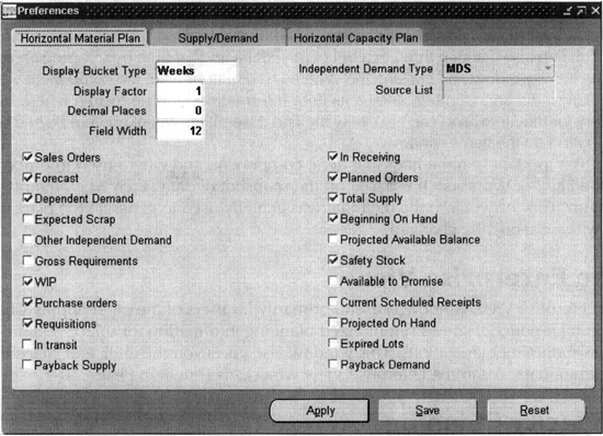
FIGURE 10-5. Preferences for the Horizontal Material Plan

Item Information

For information about the planning attributes of an item, select the Items window, as shown in Figure 10-6. This window displays items with their descriptions and the planning-related attributes that were effective when the plan snapshot was run.

FIGURE 10-6. Items window, showing item planning details

Walking Up and Down a Bill of Material

From the Items window, you can view the components of a single item by selecting the item and clicking the Components button. Separate tabs in the Components window show effectivity and quantity information, use-up information, and summarized item details. From the Components window, you can select one or more component items and access their item details (the Items window) by clicking the Items button. From there, you can view that item’s components and continue the process; in this way you can walk down the entire bill of material.

You can also walk up through a bill of material a level at time by selecting an Item on the Items window and clicking the Where Used button. As in the component view, you can select an assembly, access its item information, and perform a where-used inquiry for that item. You can also view the End Assemblies where an item is used with that button on the Items window.

It is important to remember that item, component, and where-used information on the Planner Workbench is based on the snapshot of data taken when the plan was run. This lets you see the data that was actually used to generate the plan, even if it was subsequently changed.

The Enterprise View

The Enterprise View window is useful primarily for users of the older Supply Chain Planning product; it shows summarized planning information for selected items across multiple organizations. This window also gives you the choice of snapshot or current data. A sample Enterprise View window is shown in Figure 10-7.

FIGURE 10-7. Planner Workbench Enterprise View, showing summarized planning data for multiple organizations

Capacity Planning

You can request detailed Capacity Requirements Planning (CRP) to be performed when an MRP or a DRP plan is run, using the Plan Options form shown in Figure 10-1. You check the box to enable capacity planning and optionally provide the name of a Simulation Set to reflect planning changes in capacity. As noted in Chapter 8, CRP uses detailed routing information to calculate load on your resources and compares that load to the defined capacity of those resources.

You can also perform Rough Cut Capacity Planning (RCCP) for an MPS plan type by including the name of a Bill of Resource on the plan options form. Although it lacks the detail of CRP, RCCP lets you check capacity for resources that might not be part of your routing by adding them to your bills of resource before you run RCCP. As noted in Chapter 8, you can also run Rough Cut Capacity Planning inquiries and reports against any master schedule, whether or not you included the bill of resource in your plan options.

Resource and Capacity Information

If you have requested capacity planning in your plan, you can view resource capacity information in the Planner Workbench. As noted earlier, MRP provides exception messages to identify over- and under-loaded resources. You can also view the Horizontal Capacity Plan window, shown in Figure 10-8. This window shows bucketed capacity information and can be tailored to show the data you want using the Preferences window, accessible from the Tools option on the Menu bar. You can also see detailed information about your resources on the Resources window.

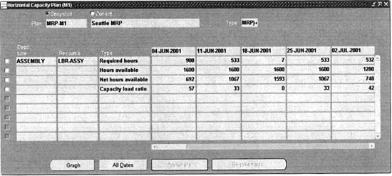
FIGURE 10-8. Horizontal Capacity Plan

Simulations

Since the introduction of the Memory Based Planner in Release 10.7, Oracle has provided the capability to simulate various changes to supply, demand, or capacity. Although sometimes referred to as “Net Change Replan” or “Net Change Simulation,” the terms can be somewhat misleading.

First, process only responds to net changes you make on the Planner Workbench itself. To many people, true net change planning means reacting to the net changes made anywhere in the ERP system—changes in inventory levels, changes to bills of material, changes to customer orders, or unplanned scrap on the shop floor. MRP net change planning does not respond to these types of changes.

Second, to the extent that changes you make on the workbench are not automatically reflected in the execution systems, the process is indeed a simulation. For example, if you simulate a change to a sales order’s schedule date, that change is not reflected on the sales order itself; it’s only stored within the specific plan you change. However, there is nothing to prevent you from implementing and executing changes you make in a “simulation” session—if you change a date on a discrete job, for example, and implement that change, it does affect the actual job.

Finally, there is no simple way to “reset” a simulation with MRP planning. You can rerun the plan and overwrite all planned orders, though that plan will then react to any subsequent changes made in the execution systems, so it will not necessarily restore the plan to its pre-simulation state. Or, you can make simulations in a copy of the plan, but depending on your planning cycle, it can be clumsy to use the simulated plan in place of the original one—if you make changes to an MPS plan, you can replace the original plan with the simulation when you run your next MRP, but if you make changes to an MRP, you must disable the old plan and procedurally determine to use the latest copy for execution.

NOTE
These issues have been addressed with the enhanced simulation capabilities of Advanced Supply Chain planning; see Chapter 11.

Copying a Plan

Rather than making changes to your production plan directly, you might want to make a copy of that plan for simulation purposes. To copy a plan, you must have a current plan to copy from (the Source Plan), and you must define a new plan name of the same type (MRP, MPS, or DRP). This is the Destination Plan. Then, using the Launch Copy Plan form, submit the concurrent request that copies the plan.

The process runs by loading data from the flat files (operating system files) generated in the planning process under the new plan name. This has several implications:

Also, your destination plan must be empty; you cannot copy into a plan after it has been populated. You can create multiple plan names to accommodate multiple copies, or you can purge a plan when you’ve finished a simulation scenario and then re-create a new, empty plan with the same name.

For simulation purposes, you should consider the Planning Time Fence Control, Overwrite, and Append Planned Orders options of the destination plan. Normally, you will want to use the planning time fence and set the Overwrite option to Outside Planning Time Fence. This enables you to create new, firmed orders inside the planning time fence and tells the replanning process to preserve those changes. (If you did not use the planning time fence and told planning to overwrite all planned orders, you would not be able to introduce new supply in the simulation; it would be overwritten by whatever the planning process calculated as necessary.)

Simulation Scenarios

You can make the following types of changes on the Planner Workbench:

You make these changes in the Supply/Demand, Supply, or Demand window of the Planner Workbench.

Simulation Modes

You can run planning simulations online or in batch mode. Online simulation gives you immediate feedback. It enables you to simulate multiple sets of changes, without increasing database traffic. However, online simulation does not allow you to change plan options, and it locks other users out of the plan while the online planner is active.

Batch replanning does take into account changes in plan options and enables other users to access the plan while you are entering your changes.

For either type of simulation, you might first want to establish a “baseline” by saving the exception message counts from the original version of the plan. To do this, navigate to the Exception Summary window of the Planner Workbench and click the Save Exceptions button. This will save the total number of exception messages in the plan with a unique version number; you can then compare the number of exceptions from the saved version(s) with the number of exceptions generated by your current simulation.

Online Simulation

To begin an online simulation session, select the Online mode in the Net Change Replan section of the Planner Workbench. Click the Start button; this launches a concurrent process that loads existing planning data into memory. You will see a status window that shows the progress of this process. See Figure 10-9 for an example.

FIGURE 10-9. Online Planner Status, ready for planning

When the process completes, you will see the status Ready for planning. At this point, you can make your changes. Enter the data you want to change and save your changes. When you have completed a set of changes and want to see the results, return to the first window of the Planner Workbench and click the Plan button.

The status window will again show you the progress of the replanning process. When the status shows Ready for planning, you can view the results—new exception messages, new planned orders, or new recommendations—on the appropriate windows.

You can continue making additional changes and replanning as necessary. When you have finished, return to the first window of the Planner Workbench and press the Stop button. This will terminate your online planning session and make the plan accessible to other users.

Batch Simulation

To perform a batch simulation, simply make the changes you want on the appropriate windows of the Planner Workbench. When you have entered all the changes you want, return to the first window of the Planner Workbench. Select Batch mode in the Net Change Replan section. Click the Plan button; this launches the concurrent process that performs the replanning. This will clear your screen; when the process is complete, re-query your plan to see the results.

Comparing Simulated Scenarios

To compare simulated scenarios in MRP planning, the only online tool available is to view the count of exception messages. If you have saved the earlier message counts, you view the number of messages by version on the Exception Summary window. Using this method, you can quickly determine whether the number of late orders has increased or decreased due to the changes you made, for example. However, you can only see the details of the current set of exceptions; you cannot see the details of the earlier versions of your exception messages.

If you have maintained separate copies of different simulation scenarios, you can compare those with the Master Schedule Comparison report.

NOTE
Simulation capabilities, and the tools available to compare various simulations, are greatly improved in Advanced Supply Chain planning, described in the next chapter.

Technical Overview of the Planning Process

At a high level, the planning process involves two types of activities—the Memory Based Snapshot copies all appropriate ERP data, and the Memory Based Planner performs the netting and planning. Since Release 10.7, Oracle has utilized its memory-based planning engine to generate MRP plans. This technology offers significant efficiency improvements over the previous planning engine—all snapshot data is read into memory before netting and order planning, and both the deletion of data from a previous plan and the loading of data from the new snapshot have been moved out of the critical path.

In reality, these two major activities are broken into a number of subprocesses; this section provides a brief overview of these processes.

Memory-based Snapshot

The overall snapshot process copies the appropriate data from the transaction systems into tables used by planning. This data includes items, bills, safety stock levels, discrete jobs, purchase orders, sales orders, etc.

The Memory-Based Snapshot program (MRCNSP) begins the process; its job is to prepare a list of planned items. While the snapshot is reading the items for the plan, a separate Snapshot Delete Worker (MRCSDW) is deleting data old snapshot data. Performing these two tasks in parallel improves performance. When the old data is deleted, the new data is loaded into the table MRP_SYSTEM_ITEMS.

At this point, the memory-based snapshot launches the Snapshot Monitor (MRCMON), which controls the remaining snapshot processes. The snapshot monitor launches one or more Snapshot Workers (MRCNSW) and the first of several Snapshot Delete Workers. This delete worker will, in turn, launch additional delete workers to delete other existing planning data, while the snapshot workers are gathering the current data. As with the memory-based snapshot itself, the deletion of old data is performed in parallel with the snapshot of the new data. The snapshot workers write data to flat files in the operating system and store the filename and location in the database table MRP_FILES.

When the old data has been deleted and the new data collected for a given planning database table, the snapshot monitor launches a Loader Worker (MRCSLD) to load the data from the snapshot files back to the database. One loader worker is launched for each planning table to be loaded. The loader workers use SQL*Loader to load the flat file data to the database. The profile MRP:Use Direct Load Option controls whether SQL*Loader will use the direct path load or the conventional path load. The conventional path load builds standard SQL INSERT statements to update the database and can be used while other plans are running. The direct path load bypasses the standard SQL processor; it is therefore much faster, but requires exclusive write access to the table that it’s loading, so that no other plans can be generated or executed.

Memory-based Planner

The Memory-Based Planner (MRCNEW) performs the planning calculations. It reads the data from the snapshot files into memory, performs planning for the list of planned items, and writes its results to another set of flat files in the operating system. At the completion of the planning process, it launches loader workers to load the final plan data back to the database.

Inter-Process Communication

The snapshot monitor uses the database table MRP_SNAPSHOT_TASKS to communicate with the snapshot delete workers. First, the snapshot monitor populates this table with a list of all the delete tasks. Each row in this table initially has a null value for START_DATE and COMPLETION_DATE. The delete workers look for the next task with a null START_DATE; a delete worker sets the START_DATE to show that it has begun to process the task and sets the COMPLETION_DATE when it is finished.

To communicate with memory-based snapshot and snapshot workers, the snapshot monitor uses database pipes. This type of communication includes requests for new snapshot tasks, task completion messages, lock requests, etc.

Concurrent Manager Requirements

With so many processes running in parallel, it is important that the concurrent manager that will run your plan can handle the number of processes your plan requires. If you run the plan as a single-threaded process, at least four concurrent processes must run simultaneously:

The first three processes will all be running simultaneously for some period of time; they cannot complete until the loader workers and snapshot workers complete their processing. Therefore, if there are only three slots (target processes) available in the concurrent manager, the process will hang.

As described earlier, you can improve performance by running the snapshot processes in parallel. You control the number of parallel processes with the profile MRP:Snapshot Workers. Setting this profile to zero runs the plan as a single-threaded process; increasing the number of workers determines the degree of multi-threading. Each snapshot worker uses a simultaneous delete worker, so two processes can be running at the same time for each snapshot worker launched. Therefore, the minimum requirements on the concurrent manager can be calculated with the following formula:

Target processes = 4 + (2 * <number_of_snapshot_workers>)

Keep in mind that these are minimum requirements; if you are running other programs in the same concurrent manager, planning can easily fill up available concurrent manager slots and impair the performance of other requests. You might want to create a separate concurrent manager for planning, or at least ensure that the concurrent manager you will use has sufficient Target Processes to accommodate planning as well as other programs you anticipate running at the same time.

Summary

This chapter discussed the unique features of unconstrained, non-optimized planning. It described the different types of plans (MRP, MPS, and DRP) and discussed how to set up and generate those plans. It also covered the factors that control the scope of a plan’s regeneration. The chapter described the available reports. The functions of the Planner Workbench for reviewing and implementing planning suggestions, viewing item and pegging information, and simulating changes to a plan and assessing the results were also covered.

This chapter has also provided a brief technical overview of the planning process. The next chapter discusses the capabilities provided by Oracle Applications to model multiple-organization, multiple-enterprise supply chains, and discusses the unique features of the newer Advanced Supply Chain Planning process.