CHAPTER 11
Advanced Supply Chain Planning

Starting with Release 11, Oracle has offered Advanced Supply Chain Planning (ASCP) as an alternative to the single-organization planning discussed in Chapter 10. As its name suggests, ASCP plans across your supply chain and can incorporate customer preferences and supplier capacity. Some of these capabilities are also present in the earlier Supply Chain Planning (SCP) product, available since Release 10.7.

This chapter highlights the differences between SCP and ASCP. It describes the tools to define your supply chain; for the most part, these tools apply to both SCP and ASCP, but differences are noted. Additionally, this chapter discusses constraint-based and optimized planning, the mechanics of defining and running plans, and the tools to view and implement the resulting recommendations. Finally, the chapter describes the integrated performance measurement tools.

What’s Different?

ASCP offers a number of enhancements to traditional planning: It offers the option of planning to material or capacity constraints; it provides automatic optimization of plans to meet explicit and implicit objectives; and it features built-in performance measurements to help you judge the effectiveness of the plan. As noted in Chapter 1, ASCP supports the concept of holistic planning—one plan can support all the functions traditionally provided by different plan types, planning all time periods, all manufacturing methods, and all organizations across the entire supply chain. This single-plan approach eliminates the synchronization of multiple plans, and it helps improve manufacturing flexibility and velocity.

As part of the holistic concept, ASCP can consolidate data from multiple instances—different instances of Oracle applications since Release 10.7, and even non-Oracle ERP systems—and provide a single, unified plan. This capability requires a much different architecture than the MRP planning (described in Chapter 10).

Multiorganization Planning

ASCP and SCP allow you to model complex supply chains and provide a unified plan for the entire supply chain. Your model can include customer preferences (for example, which organizations can supply which customers), multiple manufacturing and distribution organizations within your enterprise, and your suppliers. In simple cases, you might be able to model your supply chain using item and organization attributes. For more elaborate supply chains, you can define sourcing rules and bills of distribution and apply different sets of assignments of those rules.

The tools for defining your supply chain are described later, in the section titled “Modeling the Supply Chain.”

Constraints

Unlike Oracle MRP planning, ASCP can respect various constraints on your production and distribution capabilities. This capability, sometimes called finite planning or constrained planning, enables you to generate a plan respecting material constraints, capacity constraints (including both manufacturing resource and transportation capacity), or both. You can plan for detailed or aggregate resources, and you can use item routings or bills of resource to control the granularity of the planning process.

You can enforce constraints selectively across the planning horizon. It may be important, for example, to recognize material and capacity constraints in the near term to avoid creating a plan that you can’t execute. But at the far end of the horizon, it may be more important to generate an unconstrained plan to determine how much additional capacity you might need to meet the anticipated demand.

Constraint-based planning is a prerequisite for optimized planning—if there are no constraints, the assumption is that you can do anything; there’s nothing to optimize.

Optimization

ASCP includes the option to generate an optimized plan. In an optimized plan, the planning process determines the relative cost of the different options available to it and chooses the “best” alternative based on those costs. Some of those costs are naturally present in your ERP data, such as the cost of using a substitute item or an alternate resource. Other costs are computed in planning by applying penalty factors to different events. For example, you might assign a penalty factor of 50 percent to exceeding resource capacity (reflecting that you would pay time-and-a-half if you had to work overtime); you might assign another penalty factor to satisfying a late demand, to artificially add cost to late production. In addition, optimization is influenced by the weight you give to each of three explicit planning objectives: Maximize Plan Profit, Maximize On-Time Delivery, and Maximize Inventory Turns.

Holistic Planning

The term holistic planning was coined by Oracle to suggest that one plan could meet all the needs typically addressed by multiple plans in more traditional planning scenarios. Holistic planning eliminates or reduces the need to keep multiple plans in synch. Specifically, holistic planning accommodates three dimensions of the planning problem:

Plan Types

ASCP uses basically the same plan types as traditional MRP, but uses slightly different names:

Integrated Performance Management

ASCP incorporates performance management features from Oracle’s Business Intelligence System (BIS). The Planner Workbench for ASCP displays four Key Performance Indicators (KPIs) for each plan:

Release 11 i.5 ASCP provides additional KPIs; right-click the workbench to select the following indicators:

You can use BIS to define targets for each of these KPIs. The Planner Workbench displays a graph for each of these KPIs and their targets so that you can easily assess the effectiveness of a particular planning strategy.

ASCP also provides enhanced exception messages and uses Oracle Workflow to provide notification and response processing for all those exceptions. See the sections titled “The ASCP Planner Workbench” and “Performance Management” for examples and more details of both KPIs and exception messages.

Architecture

ASCP is able to run on a separate server from your ERP system. This architecture eliminates any performance degradation on your transactions systems when a plan is running, and it enables you to run plans more often and more quickly than with traditional planning systems. (If you will run your plans overnight or at nonpeak hours, you can use the same server for both ASCP and ERP.)

The separate-server architecture also facilitates planning for multiple ERP systems; you can define multiple ERP instances to plan, collect their data to the planning server, and then run one single, consolidated plan with the aggregate data.

Because planning is designed to run on a separate server from ERP, you must explicitly publish the planning data back to the source instance to perform certain activities in your ERP system. The Push Plan Information concurrent program provides this function. For example, if you want to create flow schedules (described in Chapter 16) from an ASCP plan, you must run this program.

Whether you run ASCP on a separate machine, a single machine, or the same database instance as your ERP system, the process of setting up and running ASCP plans is unchanged—you must still define the source instances that planning will use (described in the section titled “Defining Instances”), and you must still collect data from those instances to the planning server (described in the “Data Collection” section).

Modeling the Supply Chain

ASCP (and earlier SCP) offers several methods of representing your supply chain. For the most part, these methods are identical whether you use them with ASCP or SCP; differences are noted.

Very simple supply chains—where one product is always supplied by a single plant and where there is no need to split purchase orders between suppliers—can be modeled with the item and organization attributes discussed in Chapters 2, 3, and 8. An item’s Make/Buy attribute, for example, determines if the item is manufactured or purchased. The item’s Source Organization identifies a single source of supply within your enterprise, for example, a manufacturing plant that might supply the item to a distribution center.

To model more elaborate supply chains, where one item may have multiple or alternate sources of supply, see the section “Multiple Sourcing Options” later in this chapter.

Multiple Organization Model

Central to any form of supply chain planning is the ability to model multiple organizations within your enterprise. This topic has been discussed in Chapter 2. A single plan can accommodate one, multiple, or all the organizations in your ERP system.

When you define the ERP instances from which you will collect planning data, you must identify the organizations in those instances for which you will plan. See the section “Defining Instances,” later in this chapter. Then, when you define your plans, you define the organizations that participate in a given plan. See the “Defining the Plan” section.

NOTE
Whether your organizations use multiple sets of books or a single set of books, there is absolutely no effect on the planning process.

Multiple Sourcing Options

Oracle provides sourcing rules and bills of distribution to model multiple sources, including splitting production or purchases across plants or suppliers. These sourcing rules and bills of distribution are assigned to items, organizations, or categories using Assignment Sets. These tools allow you to model very complex supply chains; they are discussed in the following sections.

Both sourcing rules and bills of distribution use effectivity dates to let you project changes to your supply chain over time. The effectivity date initially defaults to the system date; like effectivity dates in routings or bills of material, a “null” ending date means that the effectivity of the rule has no projected end.

For each effectivity range, you define the sourcing options associated with the rule. There are three possibilities:

Though the mechanics of defining sourcing rules and bills of distribution are much the same whether you’re running ASCP or SCP, they operate very differently based on your planning method and options.

For ASCP, you assign each option a priority code. A priority code serves as a method for defining multiple sourcing scenarios—all the options within a single priority code will be considered as a unit. Within a priority code, you assign a percentage to each sourcing option. For example, if you have a group of items that you plan to buy from two different suppliers, you might define a sourcing rule with two “buy from” options within the same priority, specifying 50 percent for each supplier. If an alternate scenario for the same set of items is to buy from a single supplier, you would define a second scenario (priority) within the same sourcing rule, assigning the single supplier 100 percent of the purchases. Within a single priority code, the percentages must total 100 percent, or the group of options will not be considered by planning.

For SCP, the entire rule is treated as a single scenario; each option typically has a different priority code, which is used to “break a tie” if two options have identical planning percentages.

NOTE
This is a big difference between 10.7 SCP and ASCP. In SCP, each sourcing option typically has a different priority code, and the total of all percentages need to equal 100 percent for the sourcing rule to be active for planning.

You can define sourcing rules, bills of distribution, and assignment sets in your ERP instances; they will be collected with other planning data in the data collection process, described later. This approach makes sense if you have only one source instance, or if you want to use the same sourcing rules for other functions within your purchasing system. For example, you may want to use the same sourcing rules in your supplier item catalog that you use for planning.

You can also define sourcing rules, bills of distribution, and assignment sets on the planning server itself; this approach is useful if you will be planning for data collected from multiple ERP instances.

Sourcing Rules

A sourcing rule is a statement of planned sources of supply. Sourcing rules can be global (available to all organizations) or local (available only to the organization in which they are defined). You might use a local sourcing rule if the sourcing for a group of items varies based on the receiving organization. You might use a global sourcing rule for a set of products you buy from the same mix of suppliers, regardless of the receiving organization. A typical global sourcing rule for Global Order Promising might specify all sources of supply to your customers as “Transfer From” organizations.

Define sourcing rules on the Sourcing Rules form, shown in Figure 11-1. For each sourcing rule, specify a name and a description and choose whether the rule will be global or local.

FIGURE 11-1. Defining sourcing rules

TIP
Because you can use sourcing rules (and bills of distribution, discussed later) for many items, choosing descriptive names for the rules is helpful. For example, if you have a sourcing rule that you plan to use to identify the sources for fasteners, it might be helpful to name it something like “Fastener SR.”

In the second region of the window, specify a range of effectivity dates for the rule.

For each effectivity date range, define the sourcing options (make, buy, or transfer) and their appropriate percentages. Depending on the option you choose, enter the additional information required, as described earlier, in the section “Multiple Sourcing Options.”

Bills of Distribution

A bill of distribution is basically a collection of sourcing rules; in fact, there is nothing you can do with a bill of distribution that you could not do with a collection of sourcing rules. But based on the definition of your supply chain, using bills of distribution rather than sourcing rules may be more convenient. For example, if the same set of sourcing rules apply to a group of items regardless of their organization, it may be simpler to define one bill of distribution and assign it to the item, rather than assigning a separate sourcing rule to each item/organization.

Bills of distribution are inherently global. For each bill of distribution, you define each receiving organization and effectivity date range, then the sourcing options for each organization and date range entry, as shown in Figure 11-2.

FIGURE 11-2. Defining a bill of distribution

NOTE
Because bills of distribution and sourcing rules perform the same functions, the term “sourcing rule” is used in subsequent sections to refer to either a sourcing rule or bill of distribution.

Assignment Hierarchy

As noted earlier, sourcing rules themselves do not specify the items for which they will be used. This is the function of the assignment set and is one of the keys to the simplicity and flexibility of Oracle’s ASCP model. An assignment set is literally a set of assignments that will be used in ASCP and for the purposes of Global Order Promising. You can define multiple assignment sets and use them for different purposes. For example, you might create one assignment set for your production plan, another for a simulated plan, and another for Global Order Promising. The capability to define multiple assignment sets lets you define multiple scenarios easily and use those scenarios in different plans.

Assignment sets also simplify the process of assigning sourcing rules to your items; rather than assigning a specific rule to each item, you can assign a default to an organization or to a category of items. Assign a sourcing rule to an individual item or item/organization only to deal with exceptions. You can further qualify these assignments by customer and address (site). Figure 11-4 shows the Sourcing Rule/Bill of Distribution Assignments form.

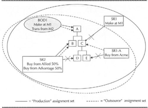
FIGURE 11-3. Assignment sets provide flexibility

FIGURE 11-4. Assign sourcing rules and bills of distribution in an assignment set

For planning, you need to define one or more assignment sets that will determine the sourcing within your enterprise.

Assignment sets simplify the setup process by allowing you to assign sourcing rules at different levels of aggregation. Assignment sets defined within your ERP instance allow the following level of assignments:

Clearly, you can reduce the setup if you can assign sourcing rules or bills of distribution by category of items, rather than assigning sourcing rules to individual items.

Assignment sets that you define on the planning server offer the following levels of assignments:

It’s possible that several assignments might apply to a given item; for example, you might have one assignment for the item and another for the category to which the item belongs. For planning purposes, the most specific assignment will be used. You can check all the assignments that exist for an item by using the View Sourcing Assignment Hierarchy, shown in Figure 11-5. This can be a good tool for troubleshooting your supply chain definition; you may find that sourcing for the item is coming from an unexpected source.

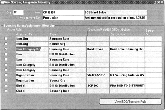
FIGURE 11-5. Troubleshoot your supply chain definition with the View Sourcing Assignment Hierarchy window

To use this form, enter the Assignment Set, Organization, Item, and effectivity date; then click the View Sourcing Hierarchy button. The resulting window shows all the levels at which you can assign sourcing information and the sourcing rule or bill of distribution that is assigned at that level. The levels are arranged in order of priority. The highest level at which sourcing information is present will be checked as Active, which indicates the sourcing information that will be used if you run a plan with this assignment set.

NOTE
The View Sourcing Hierarchy Assignments window, shown in Figure 11-5, shows that the item attribute Source Org has the second rank among all of the possible levels of source information. It overrides even sourcing rules assigned to the item across all organizations. Be careful if you set this item attribute during item maintenance because it will have a strong impact on the sourcing of the item.

Sourcing and Assignment APIs

Oracle provides two APIs to create sourcing information—the Sourcing Rules/Bill of Distribution API and the Sourcing Rules/Bill of Distribution Assignment API. Their use is described in the Oracle ASCP and Global Order Promising Technical Reference Manual, available as part of the Oracle documentation library.

Global SCP and Subset Planning

Part of the holistic planning concept is the ability to run a single, global supply chain plan. This planning strategy results in no plans to synchronize, and can greatly shorten the planning cycle. It is especially well suited to an enterprise with a centralized corporate structure, interdependence among manufacturing facilities, a common supply base, and common products.

You can also choose to plan for separate subsets of your business. For example, if one plant is the sole producer of a particular product line, you may not need to include it with other plants in your enterprise. Or if your corporate culture isn’t accustomed to global planning, you may choose to run independent plans for separate plants or lines of business; Oracle ASCP supports either approach.

Master Scheduling the Supply Chain

As noted earlier, the Production Plan, or Master Schedule, can be used to smooth production. You can generate a Production Plan, manipulate it as necessary, and then use it as input to another plan type (either a manufacturing plan or distribution plan).

Constraint-based Planning

A big difference between ASCP and earlier planning methods is the option of planning to constraints. Although Oracle has supported simultaneous material and capacity planning for a long time, the planning engine has always planned to meet due dates; capacity planning has been unconstrained, or infinite. ASCP provides the option of constraint-based planning, or finite capacity planning.

Furthermore, you can choose to plan to capacity (including transportation capacity) constraints, material constraints (including modeling the capacity of suppliers to provide material), or both; and you can specify different constraints and different levels of granularity in the different periods of the planning horizon.

Enabling Constraint-based Planning

There are two parts to enabling constraint-based planning: selecting the hard constraint and specifying the desired constraints and level of granularity across the planning horizon.

You select the hard constraint on the Options tab of the Plan Options form, shown in Figure 11-6. For each plan, you must select one of the following options:

FIGURE 11-6. Enable constraints on the Options tab of the Plan Options form

Types of Constraints

On the Aggregation tab of the Plan Options form, shown in Figure 11-7, check the Plan Capacity box. Then, identify the types of constraints and level of granularity for each portion of the planning horizon.

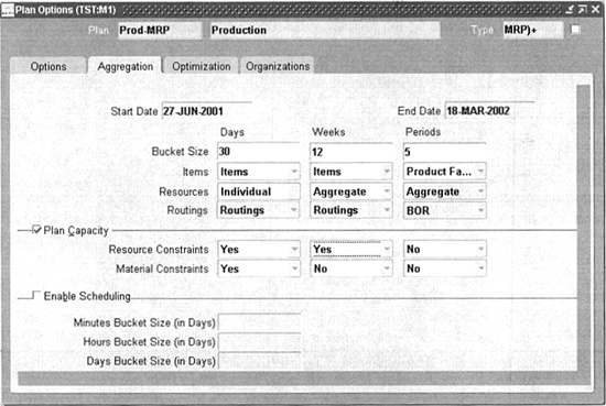
FIGURE 11-7. Identify constraints and their granularity on the Aggregation tab

For each portion of the horizon, you can choose to plan to Resource Constraints, Material Constraints, or both. Each constraint, in turn, allows you to specify the desired level of granularity by using the Items, Resources, and Routings selection on the upper section of the form:

FIGURE 11-8. Aggregate resource definition

CAUTION
Take care not to use the aggregate resource itself in your routings, or capacity planning will fail.

Modeling Supplier Capacity

If you have a good relationship with a supplier, you may be able to define and maintain the capacity they will commit to you. Planning will use this information to determine material constraints.

You can define supplier capacity by item as part of your Approved Supplier List, described in Chapter 13. Find the item/supplier combination you want and use the Attributes button to drill down to the detail. The Planning Constraints tab on the Supplier – Item Attributes window lets you specify the supplier’s capacity to produce that item, in units per day, for multiple date ranges. You can also define Tolerance Fences; for example, your agreement with your supplier may allow you to increase demand by 10 percent if you provide at least 20 days advance notice.

Workflow can route supplier capacity exception messages directly to the supplier; the supplier’s response can modify their capacity.

Optimized Planning

In addition to constraint-based planning, ASCP offers the option of optimized planning. As described earlier, an optimized plan will pick an “optimal” solution, based on the relative cost of the alternatives available. Enable optimization by checking the Optimize box on the Optimization tab of the Plan Options form, shown in Figure 11-9.

FIGURE 11-9. Enabling an optimized plan

The optimization process considers the costs of the various options and chooses the best overall alternative. As a simple example, consider the following: Suppose you have an order priced at $100. If you have assigned a penalty factor of 25 percent to a late demand, each day that you are late in meeting that demand will “cost” $25 (25 percent of the $100); thus if you’re a day late, the order will only be worth $75; if you’re two days late, the order will be worth only $50, and so on. Against this artificial cost, planning weighs the cost of various options to satisfy the demand. For example, if you could use an alternate resource to meet the demand on time, the incremental cost of that resource would be considered—if the resource cost more than $25 extra, planning might decide to ship the order one day late because the cost of the resource was greater than the penalty cost of being late.

Of course, this is a very simplistic example. Planning considers numerous other factors and many different scenarios; these factors are described briefly in the following sections, but the best advice is to test optimization carefully, changing only one factor at a time to evaluate its effect.

Optimization Objectives

Optimization uses both explicit and implicit objectives. Currently, Oracle supports three explicit objectives: inventory turns, plan profit, and ontime delivery. Implicit objectives are to minimize the costs of the following: late demand; resource and material exceptions; safety-stock violations; use of alternate sources, resources, routings, or items; and inventory carrying cost. These explicit and implicit objectives are discussed in the following sections.

Explicit Objectives

You enable each of the explicit optimization objectives on the Optimization tab of the Plan Options form (see Figure 11-9). To enable an objective, you assign a relative weight greater than 0 to the objective; a weight of 0 means the objective will not be considered. The basic data used for each of these objectives are as follows:

Implicit Objectives

Implicit objectives are to minimize a number of penalty costs. Implicit objectives each have a weight of 1, though you can control the cost by the way you choose your penalty factors. The penalty costs that planning considers include the following:

These penalty costs are calculated from existing ERP data or by applying a penalty factor to a cost. The data used includes the following:

ASCP Setup

To generate an Advanced Supply Chain Plan, you must define your supply chain, as described earlier. You must also create the flexfields used by ASCP and define the application instances for which you will plan, the demand priority rules, and the plan names and their options. The following pages describe these activities.

Create Planning Flexfields

Many of the penalty factors used by ASCP optimization are currently provided as descriptive flexfields; when you prepare to use ASCP on an existing instance, you must run the Create Planning Flexfields concurrent program to enable these flexfields. The parameters for this program allow you to choose which attribute column in each table you want to use for the appropriate penalty factor. This avoids “collision” with existing descriptive flexfields you may already be using.

Defining Instances

Because ASCP can collect and plan data from multiple instances, you must define the instances for which you will plan. You define instances on the Application Instances form.

Identify each instance with a three-character code; this code will be prepended to organization codes, sourcing rules, bills of distribution, and assignment sets that you collect to the planning server. For each Oracle instance, specify the instance type: Discrete, Process, or both. Specify the version of each Oracle instance; versions starting with 10.7 are supported. If you will collect data from a legacy system, specify its instance type as Other.

If you run the planning server in a separate instance, you must specify the Application Database Link and the Planning Database Link; these links allow communication between the application database and the planning database. Your DBA can provide these values. You can also specify a default Assignment Set for the instance.

For each instance, you must specify the organizations within the instance from which you will collect data. Click the Organizations button; you will see a list of the inventory organizations defined in the instance. Select the organizations you want to plan by checking the Enabled box next to each organization.

Demand Priority Rules

Use the Define Priority Rules to define the way ASCP should rank your demands. This will determine which demands will be given priority in an optimized plan.

For each rule, assign it a name and description; then select one or more criteria in the order in which they should be applied. Available criteria are Schedule Date, Sales Order and MDS Priority, Request Date, Promise Date, and Gross Margin. Neptune, for example, tries to satisfy its schedule dates; if multiple orders have the same schedule date, Neptune will next use the Order Priority to break a tie, followed by the Gross Margin the order will generate.

You can define as many priority rules as you want and use different rules on different plans. The Default check box lets you specify one rule as your default.

Defining the Plan

Defining an ASCP plan involves defining a plan name for the appropriate plan type and specifying the desired options. As with single-organization planning, described in Chapter 10, there are separate forms to define each plan type. Regardless of the type of plan, you give each a name and description and identify scope of organizations for which it will plan—All or Multiple. (If you select Multiple, you will identify the organizations in the plan options.) You also indicate if the plan will be used for Global Order Promising calculations and whether it is a production plan. (A production plan enables auto-release of planned orders, as described in Chapter 10.)

Basic Options

For each plan, define its characteristics on the four tabs of the Plan Options window. The Options tab was shown earlier, in Figure 11-6. Many of the options on this tab are the same as for single-organization planning and were described in Chapter 10. Options that are unique to ASCP include the following:

Aggregation

The Aggregation tab was shown in Figure 11-7. Here you set the number of daily, weekly, and period buckets for the plan; the window displays the end date of the plan based on your selections. For each bucket type, you specify the level of aggregation for that portion of the horizon. This was described earlier, in the section “Types of Constraints.”

On the Aggregation tab, you also specify whether you are planning capacity, and you select the type of constraints—resource, material, or both—that you want to recognize within each bucket type.

At the bottom of the screen, you can enable detailed scheduling for the Daily buckets within the horizon. Check the Enable Scheduling box, and then specify how many of the days within the first portion of the plan will be scheduled to the minute or hour; discrete jobs and planned orders within this portion of the horizon will be scheduled using routing information. Jobs and planned orders in the remaining portion of the daily horizon will be scheduled by day.

Optimization

The Optimization tab, shown in Figure 11-9, lets you enable optimized planning. Here you specify the weight of each explicit optimization objective and plan-level default for the following penalty factors: Exceeding material capacity percent, Exceeding resource capacity percent, Exceeding transportation capacity percent, and Demand lateness percent. Optimization objectives and penalty factors were discussed earlier, in the section titled “Optimized Planning.”

The combination of factors on the first three tabs yields a number of different classes of plans that you can define: unconstrained, resource constrained, material constrained, material and resource constrained, or optimized. But the number of options and factors that influence these plans allows for nearly infinite variety.

Plan Organizations

The Organizations tab lets you specify the scope of your plan by identifying the organizations that participate in that plan. An example of this tab is shown in Figure 11-10.

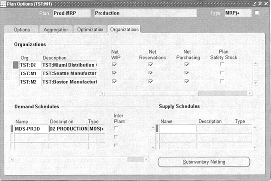
FIGURE 11-10. Planning organizations

For each organization, specify the netting and safety stock options, the same as for a single-organization plan (see Chapter 10). Include a Bill of Resource name, if you are using bills of resources (instead of detailed routings) at any point on the planning horizon. Also specify a Simulation Set if you want to recognize capacity changes as described in Chapter 4.

Specify the demand and supply schedules to be used at each organization. As described in Chapter 8, demand schedules identify independent demand. Supply schedules are used to smooth or manipulate production schedules by defining planned production for a particular organization; see “Master Scheduling the Supply Chain,” earlier in this chapter.

Data Collection

The ASCP architecture requires that data be collected from your ERP system(s) to run a plan. After a plan is generated, the appropriate data can be published back to the appropriate source instances in the form of order releases, reschedules, and cancellations.

Data collection gathers data from the organizations of your defined instances; this data is referred to in Oracle documentation as the Application Data Store (ADS). The collection process consists of two concurrent programs: Planning Data Pull and Planning ODS Load. Oracle provides a report set, called Planning Data Collection, to run these two programs sequentially.

Data collection is a two-step process to accommodate the situation where you need to perform additional data cleansing to consolidate data from various instances. Oracle automatically consolidates the following data, based on the criteria listed in Table 11-1.

TABLE 11-1. Data Consolidation Criteria

If data from multiple instances should be consolidated, even if the specified criteria do not match exactly, you can write your own programs to cleanse the data before running a plan. For example, if one source instance refers to a customer as “Oracle,” and another uses “Oracle Corporation” to identify the same customer, you might want to incorporate additional data cleansing so that both customer records are represented as the same entity.

Types of Collection

When you run data collection, you can request the categories of data you want to collect. You can run data collection as a complete refresh or in an incremental mode. Requesting a complete refresh will delete data that you have already collected for the specified instance before populating new data. Thus, if you request a complete refresh but do not request to reload a certain category of data, you will effectively remove that data from the planning process.

Running Collections

Run data collection by selecting the Planning Data Collection report set from the menu. As noted earlier, this report set consists of the Planning Data Pull and Planning ODS Load programs. Enter the desired parameters for each program.

For the Planning Data Pull program, you must identify the instance from which you will pull the data, whether you are requesting a complete refresh, the number of workers, and the language. You also identify the categories of data you want to collect; Figure 11-11 shows many of the categories of data you can choose.

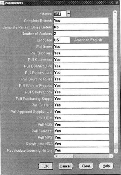
FIGURE 11-11. Planning data pull parameters

In addition to the specific categories of data, there are three additional parameters:

When you have entered the parameters for the Planning Data Pull program, enter the following parameters for the Planning ODS Load program (most often, the defaults will be appropriate): Instance, Number of Workers, Recalculate NRA, and Recalculate Sourcing History.

When the data collection process completes, you can view the collected data on the Collection Workbench. This is very similar to the ASCP Planner Workbench, discussed later in this chapter, but keep in mind that it shows only the data as collected from the source instances; no planning has taken place yet.

Running the Plan

Launching an ASCP plan is very similar to launching an MRP plan. You can access the appropriate launch form from the menu or from the Names form for the type of plan you want to run.

Plan parameters include the Plan Name, Launch Snapshot, Launch Planner, and Anchor Date. These are the same as the parameters for an MRP plan, described in Chapter 10.

The ASCP Planner Workbench

The Planner Workbench (PWB) is still the primary tool for viewing, modifying, and implementing the suggestions resulting from the planning process. Compared to the MRP Planner Workbench, the ASCP Planner Workbench has a greatly improved user interface—it provides easier access to data, a graphical view of each plan’s KPIs, enhanced drill-down capabilities, more logical display of exceptions and related exceptions, context-sensitive folder forms to display exception details, and additional options to tailor the workbench to an individual user’s preferences. It is designed to let you quickly determine priorities, view detailed information, simulate changes, and release or reschedule orders when you are satisfied with the result.

There are multiple ways to select the information you want to view:

The PWB consists of two panes: the left pane (the Navigator) presents a hierarchical display of all plans and their planned objects (such as organizations, items, resources, suppliers, and projects); the right pane displays various detailed information about the objects selected in the left pane. An extensive set of preference settings let you tailor the display to your liking.

Left Pane (Navigator)

The left pane of the Planner Workbench, called the Navigator, displays all the planned objects for all plans, arranged in six different hierarchies. You select the view you want from the drop-down list at the top of the pane. An example, illustrating the Organization view, is shown in Figure 11-12.

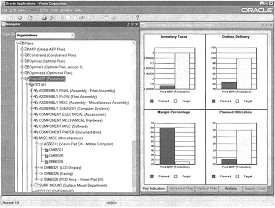
FIGURE 11-12. Planner Workbench—Organization view

The available hierarchies are Actions, Items, Organizations, Projects, Resources, and Suppliers. All views provide access to much of the same information, but the order in which it is presented differs; use the view that is most appropriate for the type of information you want. For example, if you are interested in a particular item across your enterprise, you might use the Items view; if you are interested in a group of items within an organization, you might use the Organization view; and if you are interested in items from a particular supplier, you might use the Supplier view.

Right Pane

The right pane of the PWB displays information based on the objects that you select in the Navigator. You can often select multiple objects of the same type (such as multiple plans, multiple items, or multiple resources) using standard Windows conventions (SHIFT-click, or CTRL-click); the right pane displays information for all the selected objects.

The right pane provides five different tabs to display different types of information: Key Indicators, Horizontal Plan, Vertical Plan, Actions, and Supply Chain. You can select the default tab that appears when you first open the workbench; this is described later, in the “Display Preferences” section.

Key Indicators Tab

This tab, shown in Figure 11-13, displays bar graphs of the KPIs for the objects you select. For a plan, or an organization within a plan, this tab shows four KPIs—Inventory Turns, Ontime Delivery, Margin Percentage, and Planned Utilization. As you select different types of objects in the Navigator, the KPIs may change for example, if you select items, the right pane displays the Inventory Turns and On-time Delivery KPIs for that item; for a resource, only the Planned Utilization is displayed. Additional KPIs are available in Release 11 i.5, as described earlier.

FIGURE 11-13. Planner Workbench—Key Performance Indicators

To best display the differences between the planned and target KPI values, the graphs do not necessarily start at the zero point on the Y-axis. You can expand an individual graph to the full size of the window by double-clicking; double-click again to return to the multigraph display. You can also see the precise data values by holding the mouse pointer over a bar on the graph.

For more information on the KPIs used by ASCP, see the section titled “Performance Management,” later in this chapter.

Horizontal Plan Tab

This tab displays either a horizontal material plan (for organization items selected in the left pane) or a horizontal capacity plan (if you have selected one or more resources). A sample horizontal material plan is shown in Figure 11-14.

FIGURE 11-14. Planner Workbench—Horizontal Plan

The horizontal plan displays the rows of data and the time buckets you specify in your personal preferences, discussed later in this chapter. It also displays a graph of the information.

You can expand or contract time buckets by clicking the small triangle in the label of the appropriate time period, and you can change the width of the cells by dragging the cell boundaries, much as you would in a spreadsheet. To add or remove rows of data, right-click any row label and use the Show or Hide options in the pop-up menu to modify the display. These changes are effective only as long as you have the Planner Workbench open; to make permanent changes, use the Preferences window, which you can access from the right-mouse menu.

The right-mouse menu also lets you toggle between the Horizontal View and the Enterprise View and hide or show the graph.

To scroll through the graph, click in the graph window and scroll using the left and right arrow keys. Or, you can scroll by dragging the dark gray bar at the bottom of the graph. To change the data displayed in the graph, select the rows of data you want by clicking on the button to the right of the row label in the horizontal display; you can select multiple rows with SHlFT-click or CTRL-click.

The right-mouse menu in the graph section of the window lets you select either a bar graph or line graph of the selected data.

Vertical Plan Tab

The Vertical Plan tab displays a traditional, vertical material plan in a standard folder form and a graph of the cumulative totals. The Vertical Plan tab is active only if you have selected one or more organization/items in the Navigator.

The right-mouse menu in the vertical display gives you access to the Supply/Demand and Items windows, as well as access to the standard Oracle tools for modifying the folder definition. The right-mouse menu in the graph lets you change the granularity of the display; you can choose days, weeks, or periods. Scroll this graph the same as you scroll the Horizontal Plan graph described earlier—use the left and right arrow keys or drag the dark gray bar at the bottom of the graph.

Actions Tab

The Actions tab, shown in Figure 11-15, might be considered the “heart” of the Planner Workbench for a planner or master scheduler. This tab, and its associated navigation options, was designed to make it as easy as possible for a planner to view exceptions, research the cause of potential problems, and take corrective action. This tab initially shows a summarized view of the groups of exceptions or recommendations from the plan and a graph of the number of exceptions by group. This tab is active for virtually any object selected in the Navigator and shows only the exceptions and recommendations for the selected object.

FIGURE 11-15. Planner Workbench—actions

Exception summaries are displayed in a standard folder form, which you can change as needed. The summary is arranged in order of importance—Late Sales Orders and Forecasts is at the top of the list because this is often the most serious condition; Recommendations (new orders to release) is at the bottom of the list.

Double-click a category to expand it to the specific message types within that category; a plus sign to the left of the category indicates where expansion is possible. Figure 11-15 shows the category Substitutes and Alternates Used expanded to show the specific message type, “Order sourced from alternate supplier,” in that category. Double-click a category marked with a minus sign (-) to collapse it to the summary level.

Double-click a specific message type (or use the right-mouse menu) to display the details of each instance of the message. The resulting Exception Details window uses folders specific to each message type; this allows you to display data appropriate to each message type. Like all folders, you can easily tailor the display to your liking.

For certain message types, you can use the right-mouse menu to display Related Exceptions; these are intended to help determine the cause of a problem. For example, a “Late replenishment” message might be related to a material or capacity constraint; the Related Exceptions selection on the right-mouse menu would drill directly to these related exceptions.

From the Exception Details window, you can use a button on the form to access the Supply/Demand window, where you can take action on many of the exceptions. For example, you can firm planned orders, implement planned orders, and change their dates and quantities, just as you can on the Supply/Demand window in the MRP Planner Workbench, described in Chapter 10. You can also use buttons to access the Suppliers, Items, or Resources window, based on the type of exception. The right-mouse menu lets you access additional windows for the exception, including Supply, Demand, Resource Availability, Resource Requirements, Sources, Destinations, a Gantt chart showing the schedule, and the Horizontal and Vertical Plans. Some of these additional windows are discussed in the “Additional Views” section.

Supply Chain Tab

The Supply Chain tab is active only for a single organization item selected in the Navigator. It shows you a graphical picture of the supply chain bill or a supply chain where used, starting with the selected item. This view includes sourcing information as well as bill of material information.

Additional Views

The ASCP Planner Workbench provides many additional views of planning data; a few of the most useful windows are described in the following pages.

Supply and Demand

The Supply/Demand window, shown in Figure 11-16, continues to be the “workhorse” of the PWB. This window enables you to firm planned orders, implement recommendations for new orders, and reschedule existing jobs or purchase requisitions. As you release new orders, you can firm them, modify dates and quantities, change sourcing decisions, and change the order type.

FIGURE 11-16. Planner Workbench—supply and demand

The window is organized in a tabular format.

To implement suggestions from the Supply/Demand window, check the For Release box; make any modifications using the Release Properties tab, and save your changes. Then, select Plan I Release from the menu bar. This will show a summary window of the number of jobs, schedules, requisitions, and reschedules, along with the concurrent request IDs that will implement these actions. Click OK to confirm. The Plan selection on the menu bar also includes the option to select all planned orders for release.

The Supply/Demand window includes graphical pegging information for each item if you selected pegging in your item attributes and plan options. You can access the Supply/Demand window from many places on the PWB, including the action messages, the Tools selection on the menu bar, or the right-mouse menu from the Navigator. As in the MRP Planner Workbench, individual views of Supply and Demand are also provided.

Gantt Chart

The Gantt chart provides a graphical view of your schedule. This window, shown in Figure 11-17, consists of four panes. The upper-left pane is similar to the Navigator; it lets you organize the orders or resources you want to see. The upper-right pane displays the schedules; you can reschedule jobs by dragging them to the desired point on the chart. The lower-right pane shows load and available capacity for the resources you select using the lower-left pane. Color-coding identifies resource requirements, availability, and overload, as well as resources or operation that have been updated or firmed.

FIGURE 11-17. The Gantt chart provides graphical scheduling

You can access the Gantt chart from the Supply/Demand window. Select one or more jobs or planned orders using SHIFT-click or CTRL-click; then use the right-mouse menu to access the Gantt chart for the selected orders.

Other Windows

Other windows accessible on the PWB include Item Information, Resources, Resource Requirements, and Resource Availability. These windows are accessible from the Tools selection on the menu bar or from the right-mouse menu at various places in the workbench.

You can also view the options used for a plan with the Plan I Plan Options selection on the menu bar.

Display Preferences

To access the Preferences window, select a plan on Navigator. Then select Tools I Preferences from the menu bar.

The Preferences window contains five tabs. The Other tab lets you choose the default display format for the left and right panes of the workbench. It is where you specify the default Job Status, Job Class, and Firm flag for discrete jobs you release and the grouping method for releasing requisitions. Here you can specify whether you want to release jobs for phantom or configured assemblies. This tab also lets you specify the category set you will use and filter the recommendations you see—you may want to view only recommendations for the next week or two, as opposed to viewing all the recommendations over the entire planning horizon. Finally, this tab shows the date of the snapshot and plan.

The Material Plan, Capacity Plan, Supplier Plan, and Transportation Plan tabs let you control the formats of the respective horizontal plans. You can choose the number and type (days, week, or periods) of the display buckets, the display factor (to adjust for very large or very small numbers), and the rows of data displayed.

Typical Scenarios

The possible scenarios for different exception conditions and possible resolution are virtually endless. This section lists just a few types of exception and messages and discusses possible resolution activities. The Release 11 i.4 User’s Guide, part of Oracle’s documentation library, lists each exception message and possible actions.

Late Replenishment for Sales Order

This exception is generated only for constrained and optimized plans when the Enforce Capacity Constraints option has been selected. The message details show the potential late orders. You might sort the details in descending order of Days Late to identify the most urgent orders.

You can drill to related exceptions (using the right-mouse menu) to see if the delay is the result of a combination of constraints—material, capacity, or transportation. If so, you might want to attempt to relieve these constraints, by expediting material, adding additional capacity (such as working overtime) or outsourcing production if possible. Performing a simulation of these possible solutions can help determine if they will resolve the problem.

You would perform similar actions for a “Late replenishment for Forecast” exception, although the situation is not usually as critical as a late sales order.

Constraints

Material constraint and Resource constraint messages are generated for constrained and optimized plans. You should determine the impact of the constraint; drilling to related exceptions can help. For example, if the constraint would result in a late replenishment for a sales order, it is most likely a higher priority than if it would simply delay replenishing safety stock.

You can deal with constraints in a number of ways—you might consider alternate resources or materials, adding resource capacity, modifying sourcing rules (such as using an alternate facility that has excess capacity), or outsourcing. You can simulate some of these changes on the Planner Workbench to assess their effectiveness; on an ongoing basis, you should make permanent changes in your source instances.

Reschedules

This type of exception includes Reschedule in, Reschedule out, and Past due order messages; they are generated for all plan types. The exception details show the specific order for which the exception was raised.

From the Exception Detail window, you can drill to the item’s Supply/Demand window; there you might look at the pegging information to determine what other orders are affected. (Remember: The planning process assumes that you will accept its recommendations, so if you do not act on a Reschedule in message, another order might experience a shortage.)

If you elect to reschedule the order as suggested, you can do this for most order types from the Supply/Demand window. You must reschedule purchase orders from the Purchasing application because they usually represent a contract with the supplier.

Simulations

Like single-organization planning, described in Chapter 10, ASCP allows for online simulations to evaluate the effects of changes to your plan, or different planning scenarios. For comparison purposes, you may want to make a copy of a plan before simulating changes; you can access the Copy Plan program from the main menu, or from the Planner Workbench itself, by selecting Plan I Copy Plan from the menu bar.

The ASCP Planner Workbench provides the capability to compare plans by viewing their KPIs or action messages. It also provides the capability to “bookmark” the plan at various points in the simulation process and easily restore a plan to its state at a specified bookmark.

Simulation Scenarios

As with single-organization planning, you can make a number of changes on the PWB and run a replan to see the results. The type of changes you can simulate include those listed in Chapter 10—you can add new demand or supply, modify dates or quantities, cancel orders, select alternate bills or routings, and modify resource capacity. With ASCP, you can also simulate changes to demand priorities, supplier capacity, and optimization objectives.

Simulation Modes

You can run simulations online or in batch mode, as described in Chapter 10. But unlike Oracle MRP, ASCP keeps track of the changes you make during a simulation; you can access this log by selecting Plan I Undo Summary from the menu bar. This selection opens a window that summarizes the changes you have made during a simulation session; you can view the details of a specific change with the Detail button in that window.

From the Undo Summary window, you can undo selected changes. Select one or more changes (using SHIFT-click or CTRL-click if necessary), and click Undo. You must then rerun the online planner to replan, based on the restored data. You can also create “bookmarks” at multiple points during the simulation process—select Plan I Add Undo Bookmark from the menu bar, or use the Add Bookmark button in the Undo Summary window. You will be asked to supply a name for the bookmark. You can undo all changes back to a specific bookmark by selecting that bookmark in the Undo Summary window and clicking the Undo button.

Comparing Simulated Scenarios

If you have performed your simulation in a copy of your original plan, you can compare the copy to the original, using both the KPIs and the specific action messages. This is intended to provide easier analysis of the simulation than the tools provided with older, single-organization planning.

To perform this comparison, select two or more plan names on the Navigator (left pane) of the workbench; the Key Indicators and Actions tabs will display data for all the selected plans. Figure 11-18 shows KPIs for two plans.

FIGURE 11-18. Planner Workbench—comparing the results of a simulation

You can also compare the simulation results with the original plan by comparing the count of the exceptions messages generated from each scenario. Select Plan I Save Actions from the menu bar, or select Save Actions from the right-mouse menu on the Actions tab of the Planner Workbench.

Performance Management

As mentioned earlier in this chapter, ASCP is integrated with Oracle BIS. The performance measurements provided promote continuous improvement throughout your enterprise.

Exception messages are another indicator of performance; the capabilities of the Planner Workbench to drill to the cause of an exception and take corrective action when necessary also aid in performance improvement.

Key Performance Indicators

Four KPIs are displayed on the Key Indicators tab of the Planner Workbench; see Figure 11-13 for an example. You can set targets for each of these KPIs in the Performance Management Framework within the BIS application; within BIS, KPIs are referred to as performance measures. Set the performance measures at both the Total Organizations and Total Time dimensions for the following KPIs:

You can find detailed formulas for these indicators in the Oracle Advanced Supply Chain Planning, Oracle Risk Optimization, and Oracle Global Order Promising User’s Guide—part of the standard Oracle documentation library.

Exception Messages

Release 11 i.4 provides more than 40 exceptions and recommendations; these messages are described in great detail in the User’s Guide, along with a suggested course of action for each message. Exceptions are displayed on the Actions tab of the Planner Workbench, sorted in approximate order of severity. As described in the section titled “The ASCP Planner Workbench,” many exceptions let you drill to the supporting detail and related exceptions to more easily determine the root cause of a problem.

In addition, Oracle provides five Workflow exception processes to route the appropriate information to the right people, including your trading partners. You can tailor these workflow processes to your business and trigger other workflow activities based on the responses to the notification that Workflow provides.

The seeded Workflow processes are the following:

Notifications are only generated from plans that are designated as “production.” You launch these notifications from the Planner Workbench using the Tools I Launch Notifications selection on the menu bar. Planners can view their notifications from the Planner Workbench using Tools I Notifications.

Summary

This chapter has described what makes ASCP different from standard planning—the multiorganization capability, constraints and optimization, holistic planning, and a dramatically different architecture. It has explained the tools and processes for modeling your supply chain; those tools and processes apply to older SCP as well.

The options and setup for constraint-based and optimized planning, as well as the basic setup needed to make ASCP work, have also been detailed. Additionally, the process for collecting data and launching a plan, and many of the new features of the Planner Workbench, including enhanced simulation tools, have been described.

Finally, this chapter has outlined the performance management tools—KPIs and Workflow—that Oracle has integrated with the planning process. But this chapter has just scratched the surface—Oracle advertises the simplicity of ASCP and promises rapid return on your investment. Indeed, ASCP can deliver significant benefits with minimal setup, and in very short order; the tools are straightforward. However, becoming an expert on ASCP, totally understanding all the available options, and tuning it for your enterprise can require a good deal of experimentation. Be sure to allow sufficient time for testing when you implement ASCP for the first time.