
Error Coding Techniques
5.1 Overview
Architectural vulnerability analysis, which was described in Chapters 3 and 4, identifies the most vulnerable hardware structures that may need protection. This chapter discusses how to protect these vulnerable structures with error coding techniques. The theory of error coding is a rich area of mathematics. However, instead of delving deep into the theory of error coding techniques, this chapter describes coding techniques from a practitioner’s perspective with simple examples to illustrate the basic concepts. Examples of common error codes used in computer systems and covered in this chapter include parity codes, single-error correct double-error detect (SECDED) codes, double-error correct triple-error detect (DECTED) codes, and cyclic redundancy check (CRC) codes. This chapter also discusses advanced error codes, such as AN codes, residue codes, and parity prediction circuits, which protect execution units.
For practitioners, implementation overhead of such codes is an important metric, which is also discussed in this chapter. Protecting structures from multibit faults becomes important as the structure grows in size. This chapter describes a technique called scrubbing, which can reduce the SER without incurring the overhead of the larger multibit fault detectors, and discusses how architecture-specific knowledge can reduce the overhead of error detection, help identify false errors, and help create hardware assertions to detect faults in a processor or a chipset.
Finally, this chapter discusses the role of a machine check architecture (MCA), which is invoked when the hardware detects a fault or corrects an error.
5.2 Fault Detection and ECC for State Bits
This section describes some simple, yet powerful, fault detection and error correction schemes. First, basics of error coding are described with simple examples. Then a number of coding schemes, parity codes, single error correction (SEC) codes, SECDED codes, and CRC codes, are discussed. There are other and more complex codes available, but the reader is referred to Peterson and Weldon [15] for further reading on error coding theory.
5.2.1 Basics of Error Coding
Coding schemes are one of the most powerful and popular architectural error protection mechanisms used in computing systems today. Coding schemes can be used to detect or correct single-bit or multibit error. If a fault in a bit is always detected by a code, then the bit’s SDC AVF is zero, but the DUE AVF can still be nonzero. In contrast, if a fault in a bit is not only detected but also the corresponding error is corrected by a code, then both its SDC and DUE AVFs can be made zero. First, this section illustrates the basics of single-bit fault detection and error correction using simple examples. Second, it elaborates on how the concept of Hamming distance relates to the number of errors that can be detected or corrected. Finally, it discusses the computation of the minimum number of code bits needed to correct a given number of errors in a set of bits.
Simple Examples to Illustrate Single-Bit Fault Detection and Error Correction
The basic idea of error codes can be explained with a simple example. Assume that one data bit needs to be protected against single-bit errors during its residence in a buffer (Figure 5.1). The value of this data bit can be either zero or one. Let us add one code bit to the data bit to form a code word, such that the code word is a tuple: <data bit, code bit>. Each entry of the buffer will hold such a code word. Let us define an encoding scheme that sets the code bit as follows:
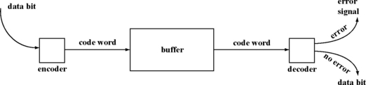
Before writing the data bit into the buffer, the encoder creates the code bit, appends it to the data bit, and writes the code word into the buffer. When the data bit needs to be read out of the buffer, the whole code word is read out and decoded. The valid code words must be either 00 or 11 since the code bit must equal the data bit. In such a case, there is no error, and the data bit is returned. However, if the code word read out is either 01 or 10, then the value of the code word changes while it was resident in the buffer. One of the causes of this bit flip could be due to an alpha particle or a neutron strike either on the data bit or on the code bit.
The decoding process is easier for code words that are separable. A code word is separable if the data bits are distinct from the code bits within a code word. For example, in the above example, the code word = <data bit, code bit>. If the code word is valid, the decoder simply extracts the data bit from the code word and returns it. Examples of nonseparable codes are covered later in this chapter.
The code word representation of 00 and 11 can only detect a single-bit fault but cannot correct it. For example, the data bit could be struck, so that the code word changes from a valid 00 word to invalid 10 code word. However, looking at 10 without any prior knowledge of what the data bit was, the decoder cannot determine if code word changed from 00 to 10 (data bit flipped) or 11 to 10 (code bit flipped).
Expanding the set of code bits can help identify the bit in error. For example, let us define a new code word as a three-tuple: <data bit, code bit 1, code bit 2>. Then, let us define the code bits as:
The valid code words are 001 and 110. Based on this code, one can easily identify the bit position that got struck. For example, if the code word is 101, then one can say that the data bit was struck. This is because the code bit 1 = NOT (code bit 2), which is the correct relationship. But the relationship between data bit and code bit 1 and that between data bit and code bit 2 are inconsistent. This inconsistency can arise only if the data bit experienced a fault. It should be noted that code bit 2 could be set to data bit itself (without the inversion).
For the code word defined above, determine which bit is in error when the code word is 111.
SOLUTION Code bit 2 is in error. This is because the code bit 1 = data bit = 1. But code bit 2 is not the inverse of either data bit or code bit 1.
The examples in this section illustrate the detection and correction of single-bit errors. The same basic concepts can be expanded to cover the detection and/or correction of multibit errors. Such codes are covered later in this section.
Determination of Number of Bit Errors That Can Be Detected and Corrected
As must be evident by now, code words are often divided into two distinct spaces: words that are fault-free and words that have faults in them. In our example for fault detection earlier in this section, the fault-free code words were 00 and 11 and erroneous code words were 10 and 01. Similarly, in our error correction example, the error-free code words were 001 and 110 and any other bit combination is erroneous. When one or more errors occur, the code word moves from an error-free to an erroneous space, which makes it possible to detect or correct the error.
There is, however, a limit to the number of errors a code word can detect or correct. For example, the example code word for error detection can only detect one error. However, if two bits are in error, then this code word may not be able to detect the double bit error. For example, if the first bit of the code 00 gets struck, then it can change to 10 (erroneous word). But if the second bit is struck now, it can change to 11, making it a valid code word. Consequently, this code cannot detect double-bit errors. The number of bits a coding scheme can detect or correct is determined by its minimum Hamming distance.
The Hamming distance between two words or bit vectors is the number of bit positions they differ in. For example, consider the following two words: A = 00001111 and B = 00001110. They only differ in the last bit position, so the Hamming distance between A and B is 1. If B were 11110011, then A and B differ the in the first six bit positions, hence the Hamming distance between A and B would be 6. If A and B were the nodes of a binary n-cube, then the Hamming distance would be the minimum number of links to be traversed to get from A to B.
Given a code word space, the minimum Hamming distance of the code word is defined as the minimum Hamming distance between any two valid (fault-free) code words in the space. For example, for our example code word that only detects faults, the valid code words are 00 and 11. The minimum Hamming distance for this code space is 2. Similarly, the valid code words for our error correction example are 001 and 110. The minimum Hamming distance for this code word space is 3.
Consider the following set of code words: 000, 011, 101, 110. What is the minimum Hamming distance for this set of code words?
SOLUTION Assume HD(x, y) = Hamming distance between x and y. Then, HD(000, 011) = 2, HD(000, 101) = 2, HD(000, 110) = 2, HD(011, 101) = 2, HD(011, 110) = 2, HD(101, 110) = 2. Hence, the minimum Hamming distance = 2.
The minimum Hamming distance of a code word determines the number of bit errors that can be detected and/or corrected by the code word. There are three key results:
![]() The minimum Hamming distance of a code word must be α + 1 for it to detect all faults in α or fewer bits in the code word. In our error correction example, the minimum Hamming distance of the code word was 3, with the valid code words being 001 and 110 (α = 2). Consequently, a single error or a double-bit error will convert a valid error-free code word into a code word with error. A third error, however, can potentially bring the code word back into the error-free space, thereby avoiding detection. Hence, this code word can only detect either single-bit or double-bit errors but not triple-bit errors.
The minimum Hamming distance of a code word must be α + 1 for it to detect all faults in α or fewer bits in the code word. In our error correction example, the minimum Hamming distance of the code word was 3, with the valid code words being 001 and 110 (α = 2). Consequently, a single error or a double-bit error will convert a valid error-free code word into a code word with error. A third error, however, can potentially bring the code word back into the error-free space, thereby avoiding detection. Hence, this code word can only detect either single-bit or double-bit errors but not triple-bit errors.
![]() The minimum Hamming distance of a code word must be 2β + 1 for it to correct all errors in β or fewer bits in the code word. Again, in our error correction example, the minimum Hamming distance of the code word was 3, so β = 1. Any fault in β or fewer bits will still be at least β + 1 Hamming distance from the nearest valid code word. Thus, given a valid code word 001 (in our error correction example), a bit flip in the first bit would convert it to 101, which is still at a Hamming distance of 2 away the other valid code word of 110. Thus, no other single-bit error in any bit other than the first one can reach this erroneous code word 101. Hence, the bit position in error can be precisely identified and hence corrected.
The minimum Hamming distance of a code word must be 2β + 1 for it to correct all errors in β or fewer bits in the code word. Again, in our error correction example, the minimum Hamming distance of the code word was 3, so β = 1. Any fault in β or fewer bits will still be at least β + 1 Hamming distance from the nearest valid code word. Thus, given a valid code word 001 (in our error correction example), a bit flip in the first bit would convert it to 101, which is still at a Hamming distance of 2 away the other valid code word of 110. Thus, no other single-bit error in any bit other than the first one can reach this erroneous code word 101. Hence, the bit position in error can be precisely identified and hence corrected.
![]() The minimum Hamming distance of a code word must be α + β + 1, where α ≥ β, for it to detect all errors in α or fewer bits and correct all errors in β or fewer errors. This result follows from the prior two results about error detection and correction. Thus, if the minimum Hamming distance of a code word is 4, then it can correct single-bit errors and detect double-bit errors, if α = 2 and β = 1. Such a coding scheme is referred to as SECDED codes, which are covered later in this section. Figure 5.2 shows the number of bit errors that can be detected or corrected, given a minimum Hamming distance for a code word. It should be noted that different numbers of bit errors can be detected and corrected depending on the values of α and β.
The minimum Hamming distance of a code word must be α + β + 1, where α ≥ β, for it to detect all errors in α or fewer bits and correct all errors in β or fewer errors. This result follows from the prior two results about error detection and correction. Thus, if the minimum Hamming distance of a code word is 4, then it can correct single-bit errors and detect double-bit errors, if α = 2 and β = 1. Such a coding scheme is referred to as SECDED codes, which are covered later in this section. Figure 5.2 shows the number of bit errors that can be detected or corrected, given a minimum Hamming distance for a code word. It should be noted that different numbers of bit errors can be detected and corrected depending on the values of α and β.

What is the minimum Hamming distance of a code that can detect two faults and correct one?
SOLUTION From Figure 5.2, such a code must have a minimum Hamming distance of 4.
Determination of the Minimum Number of Code Bits Needed for Error Correction
There is an alternate formulation that computes the minimum number of code bits needed, given the number of bit errors that need to be corrected. In contrast, the formulation above shows the number of bits that can be corrected, given the minimum Hamming distance of a code word. Given k data bits and r code bits (where n = k + r), the r code bits must be able to precisely determine the bit position or positions in error. To correct a single-bit error, the 2r combinations arising from the r code bits must be able to determine where the error occurred in the n bits. This combination must also be able to represent that no bit position is in error. This results in the equation
If k = 1, then r must be at least 2 to satisfy the above inequality. Thus, in our error correction example above, the number of code bits chosen (two) was optimal.
The number of error correction bits used determines the code’s storage overhead. Figure 5.3 shows how this overhead grows with the number of data bits for single-bit error correction. The overhead of single-bit error correction decreases with the increase in the number of data bits. For example, for a single data bit, the overhead of error correction is 200%. In contrast, for 64 data bits, only 7 code bits are necessary for single-bit correction, which results in an overhead of only 11%. However, the number of data bits that can be covered in a single code word depends on a variety of implementation issues, such as the number of available data bits, timing. Implementation issues for ECC are discussed later in this section.

FIGURE 5.3 The minimum number of code bits needed to correct a single-bit error for a given number of data bits.
The minimum number of code bits required to correct multiple bit errors can be computed in a similar fashion. To correct a double-bit error, for example, the number of code words must cover the following three cases: no error (1), single-bit errors (k + r), and double-bit errors (k+r)C2.1Hence, one has the inequality:
Thus, to correct double-bit errors in a 64-bit data word (i.e., k = 64), r or the number of code bits must be at least 12. In general, the minimum number of code bits (r) needed to correct m bit errors in a data word with k bits is given by
Using the above equation, compare the increase in storage overhead to correct a single-bit error, a double-bit error, and a triple-bit error in a 64-bit data word.
SOLUTION For all three correction schemes, k = 64. For a single-bit correction (m = 1), the minimum r = 7. For a double-bit correction (m = 2), the minimum r = 13. For a triple-bit correction (m = 3), the minimum r = 20. Consequently, the overheads for single-bit, double-bit, and triple-bit corrections are 11%, 22%, and 32%, respectively.
A designer usually carefully weighs these overheads in error correction against the performance degradation the chip may experience. For example, a processor cache often occupies a significant fraction of the chip. For a single-error correction (SEC), the overhead is about 11%, whereas for a triple-error correction, the overhead is as high as 32%. An overhead of 11% indicates that about 10% (= 11/111) of the bits available for a cache are used for error correction. Similarly, a 32% overhead indicates that about 24% (= 32/132) of the bits available for a cache are used for error correction. Thus, going from a single-bit correction to a triple-bit correction, about 14% more bits are needed. Instead of using these bits for error correction, these bits could be used to increase the performance of the chip itself by increasing the size of the cache. The designer must carefully weigh the advantage of a triple-error correction against increasing the performance of the chip itself.
The next few sections describe different fault detection and error correction strategies and the overheads associated with them.
5.2.2 Error Detection Using Parity Codes
Parity codes are perhaps the simplest form of error detection. In its basic form, a parity code is simply a single code bit attached to a set of k data bits. Even parity codes set this bit to 1 if there is an odd number of 1s in the k-bit data word (so that the resulting code word has an even number of 1s). Alternatively, odd parity codes set this bit to 1 if there is an even number of 1s in the k-bit data word (so that the resulting code has an odd number of 1s). Given a set of k bits (denoted as a0 a1 … ak–1), one can compute the even parity code corresponding to these k bits using the following equation:
Even parity code = a0 ![]() a1
a1 ![]() K
K ![]() ak–1
ak–1
where ![]() denotes the bit-wise XOR operation.2 For example, given a set of four bits 0011, the corresponding even parity code is 0. Parity codes are separable since the parity bit is distinct and separate from the data bits.
denotes the bit-wise XOR operation.2 For example, given a set of four bits 0011, the corresponding even parity code is 0. Parity codes are separable since the parity bit is distinct and separate from the data bits.
The minimum Hamming distance of any parity code is two, so a parity code can always detect single-bit faults. Such a code can also detect all odd numbers of faults since every odd number of faults will put the code word back into the erroneous space. Parity codes cannot, however, detect even numbers of faults since two faults will put the word back into fault-free space.
Parity codes can be made to detect spatially contiguous multibit faults using a technique called interleaving. Figure 5.4 shows an example of two interleaved code words. If two contiguous bits are upset by a single alpha particle or a neutron strike, then the particle strike will corrupt both code words 1 and 2. The parity codes for the individual code words will detect the error. Interleaving distance is defined as the number of contiguous bit errors the interleaving scheme can catch. The interleaving distance in Figure 5.4 is 2. Alternatively, for example, if three code words are interleaved, such that any three contiguous bits are covered by three different parity codes, then the interleaving distance is 3. The greater is the interleaving distance for a given number of code word bits, the greater is the distance the XOR tree for the parity computation has to be typically spread out. Hence, a greater interleaving distance will typically require a longer time to compute the parity tree. Whether this affects the timing of the chip under design depends on the specific implementation.

FIGURE 5.4 Example of interleaving. Bits (represented by squares) of code words 1 and 2 are interleaved. The interleaving distance is 2.
The number of bits a parity code can cover may depend on either the implementation or the architecture. To meet the timing constraints of a pipeline, the parity code may have to be restricted to cover a certain number of bits. Then, the set of bits that need protection may have to be broken up into smaller sized chunks—with each chunk covered by a single parity bit.
In some cases, the architecture may dictate the number of bits that need be covered with parity. Many instruction sets allow reads and writes to both byte-sized data and word-sized data. A word in this case can be multiple bytes. Per-byte parity, instead of per-word parity, allows the architecture to avoid reading the entire word to compute the appropriate parity for a read to a single byte. For example, a word could be composed of the following two bytes: 00000001 and 00000001. If parity is computed over the whole word, then the parity bit is 0 (assuming even parity). But if the first byte and the word-wide parity code are read, one may erroneously conclude that there has been a parity error, when there was not a parity error to begin with. Hence, to determine if the first byte had an error, the entire word along with its parity bit needs to be read out. Instead, having per-byte parity allows the architecture to only read the first byte and its corresponding parity bit to check for the error in the first byte.
The next section describes how to extend the concept of parity bits to correct bit errors.
5.2.3 Single-Error Correction Codes
Given a set of bits, a conceptually simple way to detect and correct a single-bit error is to organize the data bits in a two-dimensional array and compute the parity for each row and column. This is referred to as a product code. In Figure 5.5, 12 data bits are arranged in a 4 × 3 two-dimensional array. Then one can compute the parity for each row to generate the horizontal parity bits and for each column to generate the vertical parity bits. In such an arrangement, if an error occurs in one of the data bits, then the error can be precisely isolated to a specific row and column. The combination of the row and column indices will point to the exact bit location where the error occurred. By flipping the identified bit, one can correct the error. These codes are called product codes.

In the example in Figure 5.5, the horizontal and vertical parity bits are read out as 110 and 0100, respectively. Was there a fault? If so, which bit encountered the fault?
SOLUTION The vertical parity bits are all correct, but the second horizontal parity bit is incorrect. This implies that there was no fault in the data bits. Hence, one can conclude that the second horizontal parity bit encountered a fault. By flipping the bit to zero, we can correct it.
Product codes using horizontal and vertical parity bits are, however, not optimal in the number of code bits used. For example, to detect a single-bit error in 12 data bits, the product code in Figure 5.5 uses seven code bits. However, as Figure 5.3 shows, the optimal number of code bits necessary to correct a single-bit error in 12 bits is five. More sophisticated ECC can reduce the number of code bits necessary for SEC. To describe how ECC works, the concept of a parity check matrix is now introduced.
A parity check matrix consists of r rows and n columns (n = k + r), where k is the number of data bits and r is the number of check bits. Each column in the parity check matrix corresponds to either a data bit or a code bit. The positions of the 1s in a row in the parity check matrix indicate the bit positions that are involved in the parity check equation for that row. For example, the parity check matrix in Figure 5.6a defines the following parity check equations:

FIGURE 5.6 Parity check matrices for the code word: D1D2D3D4 with corresponding code bits C1C2C3. (a) Parity check matrix where code bit columns are contiguous. (b) Parity check matrix where the code bit columns are in power of two positions. The syndrome (discussed in the text) for (b) points to the bit position in error, if the count of the column is started from 1. The syndrome zero would mean no error.
where ![]() denotes the bit-wise XOR operation. If D1D2D3D4 = 1010, then C3 = 1, C2 = 0, C1 = 1. The corresponding code word C1C2C3D1D2D3D4 is 1011010. If E represents the code word vector, then in matrix notation, E =[1 0 1 1 0 1 0].
denotes the bit-wise XOR operation. If D1D2D3D4 = 1010, then C3 = 1, C2 = 0, C1 = 1. The corresponding code word C1C2C3D1D2D3D4 is 1011010. If E represents the code word vector, then in matrix notation, E =[1 0 1 1 0 1 0].
The parity check matrix is created carefully to allow the generation of the syndrome, which identifies the bit position in error in a given code word. If P is the parity check matrix and in E is the code word vector, then the syndrome is expressed as
where ET is the transpose of E. For example, if P is the parity check matrix in Figure 5.6a and E = [1 0 1 1 0 1 0], then one can derive S as

If S is expressed as [S3 S2 S1], then S3 = (0 AND 1) ![]() (0 AND 0)
(0 AND 0) ![]() (1 AND 1)
(1 AND 1) ![]() (0 AND 1) e (1 AND 0) e (1 AND 1)
(0 AND 1) e (1 AND 0) e (1 AND 1) ![]() (1 AND 0) = 0, where the dot represents the bit-wise AND operation and
(1 AND 0) = 0, where the dot represents the bit-wise AND operation and ![]() represents the bit-wise XOR operation. S2 and S1 can be computed in a similar fashion. The syndrome in this example is zero, indicating that there is no single-bit error in the code word E.
represents the bit-wise XOR operation. S2 and S1 can be computed in a similar fashion. The syndrome in this example is zero, indicating that there is no single-bit error in the code word E.
Any nonzero syndrome would indicate an error in E. By construction, S1 = C1 ![]() C′1
C′1![]() , S2 = C2
, S2 = C2 ![]() C′2
C′2![]() , and S3 = C3
, and S3 = C3![]() C′3, where Ci is the parity code computed before the code word was written into the buffer and C′
C′3, where Ci is the parity code computed before the code word was written into the buffer and C′![]() is the parity code computed after the code word is read out of the buffer. If any of Ci (resident parity) and C′
is the parity code computed after the code word is read out of the buffer. If any of Ci (resident parity) and C′![]() (recomputed parity) do not match, then the code word had a bit flip while it was resident in the buffer. Hence, S will be nonzero. For example, if D1 flips due to an alpha particle or a neutron strike (denoted in bold in the vector ET shown below, then one can obtain S as
(recomputed parity) do not match, then the code word had a bit flip while it was resident in the buffer. Hence, S will be nonzero. For example, if D1 flips due to an alpha particle or a neutron strike (denoted in bold in the vector ET shown below, then one can obtain S as

The reader can easily verify that the bit error in each code word position creates a different syndrome value that can help identify and correct the bit in error. More interestingly, if the check bits are placed in power-of-two positions (1, 2, 4, …) and the column count starts with 1 (zero indicates no error), then the syndrome identifies exactly which bit position is in error. Such a coding scheme is referred to as a Hamming code. The parity check matrix in the prior example is not organized as such. Thus, the syndrome is 3 although the error is in bit position 4. In contrast, the parity check bits are placed in power-of-two positions in Figure 5.6b. Using this parity check matrix and code word matrix E rewritten as [C1C2D1C3D2D3D4], one can get the syndrome as

Thus, the syndrome is three, which is also the bit position in error. This is also referred to as a (7,4) Hamming SEC code. In general, a Hamming code is referred to as (n, k) Hamming code.
Using the above parity check matrix, find the bit position in error in the code word 1010010.
SOLUTION S3 = 1, S2 = 0, S1 = 0, indicating the bit position in error is 100 or in the fourth position.
From Figure 5.2, it follows that the minimum Hamming distance of SEC codes is 3. This also implies that no two columns in the parity check matrix of a SEC code can be identical (that is, each column is unique). This is because if two columns were identical, then one can create two valid code words that only differ in ET’s bit positions that correspond to the identical columns. For example, if the last two columns are identical in the parity check matrix shown above, then one could create two valid code words, both of which have identical bits except for the last two bits. The two code words could have 00 and 11 as the last two bits. This would imply that the code word’s minimum Hamming distance is 2 and, hence, it will not be able to correct any single-bit error.
In the parity check matrix shown below, the last two columns are identical. Create two code words that when multiplied with the parity check matrix yield zero syndrome but are only apart by a Hamming distance of 2.

SOLUTION The following two code words—1001100 and 1001111—yield a syndrome of zero with the above parity check matrix but are only apart by a Hamming distance of 2. Hence, this parity check matrix will not be able to correct single-bit errors.
As may be clear by now, a SEC ECC is simply a combination of multiple parity trees (e.g., for C1, C2, and C3). By creating and combining the parity check equations carefully, one is able to detect and correct a single-bit error. Further, the code words protected with ECC can be interleaved to correct multibit errors in the same way as the code words protected with parity bits can be interleaved to detect multibit errors (as discussed in the previous section, Error Detection Using Parity Codes). For further reading on SEC and the theory of ECC spanning the use of Galois fields and generator matrices, readers are referred to Peterson and Weldon [15].
5.2.4 Single-Error Correct Double-Error Detect Code
A SEC code can detect and correct single-bit errors but cannot detect double-bit errors. As suggested by Figure 5.2, a SECDED code’s minimum Hamming distance must be 4, whereas this SEC code’s minimum Hamming distance is 3 and hence it cannot simultaneously correct single-bit errors and detect doublebit errors. For the parity check matrix for the Hamming SEC code in the previous subsection, consider the following code word with errors in bit positions 3 and 8: [1 0 0 1 0 1 1]. The Hamming SEC code syndrome is 100, which suggests a single-bit error in bit position 4, which is incorrect. The problem here is that a nonzero syndrome cannot distinguish between a single- and a double-bit error.
A SEC code’s parity check matrix can be extended easily to create a SECDED code that can both correct single-bit errors and detect double-bit errors. Today, such SECDED codes are widely used in computing systems to protect memory cells, such as microprocessor caches, and even to register files in certain architectures. To create a SECDED code from a SEC code, one can add an extra bit that represents the parity over the seven bits of the SEC code word. The syndrome becomes a 4-bit entity, instead of a 3-bit entity, for SEC codes. Then, one can distinguish between the following cases:
![]() If the syndrome is zero, then there is no error.
If the syndrome is zero, then there is no error.
![]() If the syndrome is nonzero and the extra parity bit is incorrect, then there is a single-bit correctable error.
If the syndrome is nonzero and the extra parity bit is incorrect, then there is a single-bit correctable error.
![]() If the syndrome is nonzero, but the extra parity bit is correct, then there is an uncorrectable double-bit error.
If the syndrome is nonzero, but the extra parity bit is correct, then there is an uncorrectable double-bit error.
The parity check matrix of this SECDED code can be represented as

The additional first row now represents the extra parity bit. The additional last column places the extra parity bit in the power-of-two position to ensure it is a Hamming code. Hence, the code word with the double-bit error would look like [1 0 0 1 0 1 1 0], where the last 0 represents the extra parity check bit. Then, H × ET gives us:

Here the extra bit (last bit in code word) is correct, but the syndrome 0100 is nonzero. Therefore, this SECDED code can correctly identify a double-bit error. However, if the code word is [1 0 0 1 0 1 0 0], then the extra bit is zero and incorrect, which suggests a single-bit error. The resulting syndrome is 1011, the lower three bits of which indicate the bit position in error.
The parity check matrix of a SECDED code has important properties that can be used to optimize the design of the code. Like the parity check matrix for a SEC code, all the columns in SECDED code’s parity check matrix must be unique for it to correct single-bit errors. Also, since the minimum Hamming distance of a SECDED code is 4, no three or fewer columns of its parity check matrix can sum to zero (under XOR or modulo-2 summation). This also implies that no two columns of a SECDED code’s parity check matrix can sum to a third column. These properties can be used to optimize the implementation of a SECDED ECC.
The number of 1s in the parity check matrix has two implications on the implementation of the SECDED code. First, each entry with a 1 in the parity check matrix causes an XOR operation. Hence, typically, greater the number of 1s in the parity check matrix, greater is the number of XOR gates. Second, greater the number of 1s in a single row of the parity check matrix, the greater is the time taken or complexity incurred to compute the SECDED ECC. For example, the first row of the SECDED ECC shown above has all 1s and hence requires either a long sequence of bit-wise XOR operations or a wide XOR gate. Consequently, reducing the number of 1s in each row of the parity check matrix results in a more efficient implementation. For example, the following parity check matrix (with the code word sequence [C1C2D1C3D2D3D4C4])

has only a total of sixteen 1s compared to the earlier one that has twenty 1s. Further, the maximum number of 1s per row is four compared to eight in the earlier one.
This optimized parity check matrix is based on a construction proposed by Hsiao and is referred to as the Odd-weight column SECDED code [5]. Hsiao’s construction satisfies the properties of the parity check matrix (e.g., no three or fewer columns can sum to zero) yet results in a much more efficient implementation. Hsiao’s construction imposes the following restrictions on a parity check matrix’s columns:
The parity check matrix above satisfies these properties. A zero syndrome indicates no error, but the condition to distinguish between a single- and a double-bit error is different from what was used before. If the number of 1s in the syndrome is even, then it indicates a double-bit error; otherwise it is a single-bit error. Thus, with the code word [1 0 0 1 0 1 0 0], one gets a syndrome of 1011. Since the number of 1s is odd, it indicates a single-bit error. The lower three bits specify the bit position in error. Hsiao [5] describes how to construct Odd-weight column SECDED codes for an arbitrary number of data bits.
5.2.5 Double-Error Correct Triple-Error Detect Code
As seen earlier, SEC or SECDED codes can be extended to correct specific types of double-bit errors. Interleaving independent code words with an interleaving distance of 2 allows one to correct a spatially contiguous double-bit error. A technique called scrubbing, described later in this chapter, can help protect against a temporal double-bit fault, which can arise due to particle strikes in two separate bits protected by the same SEC or SECDED code. The scrubbing mechanism would attempt to read the code word between the occurrences of the two faults, so that the SEC or SECDED code could correct the single-bit fault before the fault is converted into a double-bit fault.
The applicability of interleaving or scrubbing, however, is limited to specific types of double-bit faults and may not always be effective (e.g., if the second error occurs before the scrubber gets a chance to correct the first error). In contrast, a DECTED code can correct any single- or double-bit error in a code word. It can also detect triple-bit faults. To understand the theory of DECTED codes, one needs a background in advanced mathematics. The theory itself is outside the scope of this book. Nevertheless, using an example, this section illustrates how a DECTED code works. The construction of this example DECTED code follows from a class of codes known as BCH codes named after the inventors R. C. Bose, D. K. Ray-Chaudhuri, and A. Hocquenghem.
There are some similarities between how DECTED and SECDED codes work. Like in a SECDED code, a DECTED code can construct a parity check matrix, which when multiplied by the code word gives a syndrome. By examining the syndrome, one can identify if there was no fault, a single-bit fault, a double-bit fault, or a triple-bit fault. The minimum Hamming distance of a DECTED code is 6 (see Determination of Number of Bit Errors That Can Be Detected and Corrected, p. 164). This also implies that any linear combination of five or fewer columns of the parity check matrix of such a code is not zero.
A parity check matrix for a (N – 1, N – 2m – 2) DECTED code is usually expressed in a compact form as

where X is the root of a primitive binary polynomial P(x) of degree m, N =2m, the number of data bits is N – 2m – 2, and number of check bits is 2m + 1. The design may have to incur the overhead of extra bits if the number of data bits is fewer than N – 2m – 2.
As an example, one can define a (31, 20) DECTED code with m = 5 and P(X) = 1 + X2 + X5. In a binary vector format, X can be expressed as a vector [0 1 0 0 0], where the entries of the vector are the coefficients of the corresponding polynomial. Similarly, X4 can be expressed as [0 0 0 0 1].X5 will be computed as X5 mod P(X), which equals 1 + X2 and is expressed in a binary vector format as [1 0 1 0 0]. Expanding the Xs for the (31, 20) DECTED code, one can obtain the following parity check matrix:
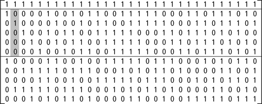
The vector X embedded in this matrix is shaded. Column 2 of this matrix is [1 0 1 0 0 0 0 0 0 1 0], which is the same as [1 X X3].
The syndrome can be obtained by multiplying the parity check matrix with the code word vector. The syndrome is a binary vector with 2m + 1 entries and can be expressed as [S0 S1 S2], where S0 consists of one bit and S1 and S2 both consist of m bits each. The syndrome can be decoded as follows:
![]() If the syndrome is zero, then there is no fault.
If the syndrome is zero, then there is no fault.
![]() If S0 = 1, then there is a single-bit fault and the error position is the root of the linear equation y + S1 = 0. The error can be corrected by inverting the bit position.
If S0 = 1, then there is a single-bit fault and the error position is the root of the linear equation y + S1 = 0. The error can be corrected by inverting the bit position.
![]() If S0 = 0, then there is a double-bit error. If the bit positions in error are E1 and E2 (expressed as numbers less than 2m), then it turns out that S1=E1+E2 and S2 = E13 + E23. It can be shown that E1 and E2 are roots of the quadratic equation S1 y2+S12y+(S13+S2) = 0. It should be noted that for a single-bit error (say with E1>0 and E2 = 0), this equation degenerates into the linear equation y + S1 = 0. This is because S13 + S2 = E12E2 + E1E22 = E1E2S1. If E2 = 0, then S13 + S2 = 0.
If S0 = 0, then there is a double-bit error. If the bit positions in error are E1 and E2 (expressed as numbers less than 2m), then it turns out that S1=E1+E2 and S2 = E13 + E23. It can be shown that E1 and E2 are roots of the quadratic equation S1 y2+S12y+(S13+S2) = 0. It should be noted that for a single-bit error (say with E1>0 and E2 = 0), this equation degenerates into the linear equation y + S1 = 0. This is because S13 + S2 = E12E2 + E1E22 = E1E2S1. If E2 = 0, then S13 + S2 = 0.
![]() If S0 = 0 and the quadratic equation has no solution or if S0 = 1 and the quadratic equation does not degenerate into a linear equation, then there is an uncorrectable error.
If S0 = 0 and the quadratic equation has no solution or if S0 = 1 and the quadratic equation does not degenerate into a linear equation, then there is an uncorrectable error.
For example, if the 31-bit code word is [000 … 0], then the syndrome is zero and there is no fault. If the code word is [100 … 0], then the syndrome is [1 1 0 0 0 0 1 0 0 0 0]. That is, S0 = 1, S1 = [10000], and S2 = [1 0 0 0 0]. Since S0 = 1, one would expect a single-bit fault. The solution to the equation y + S1 = 0 is y = 1, indicating that the bit position 1 is in error. If the 31-bit code word is [1 1 0 … 0], then the syndrome is [0 1 1 0 0 0 1 0 0 1 0]. S0 = 0, S1 = [1 1 00 0], S2= [1 0 0 1 0]. S1 can be interpreted as the number 3, and S2 can be interpreted as the number 9. The reader can verify that the first and second bit positions are in error. Then, S1 = E1+ E2 = 1 + 2 = 3. S2 = 13 +23 = 9. Instead of solving the quadratic equation in hardware to find the bit positions in error, researchers have proposed to solve the quadratic equation for all possible values of the syndrome and store the values in a table for use by the hardware.
5.2.6 Cyclic Redundancy Check
CRC codes are a type of cyclic code. An end-around shift of a cyclic code word produces another valid code word. Like the Hamming codes discussed so far in this chapter, CRC codes are also linear block codes. CRC codes are typically used to detect burst errors, errors in a sequence of bits. Typically, such errors arise in transmission lines due to coupling and noise but not due to soft errors.
Soft errors usually do not affect transmission lines because metal lines transferring data can typically recover from an alpha particle or a neutron strike. Nevertheless, CRC codes can provide soft error protection for memory cells as a by-product of protecting transmission lines. For example, if there is a buffer into which the data from a transmission line are dumped before the data are read out and the CRC is decoded, then the buffer is protected against soft errors via the CRC code. CRC codes by themselves only provide error detection, so the CRC code reduces the buffer’s SDC AVF to close to zero. However, often when a CRC error is detected by the receiver, it sends a signal back to the sender to resend the data. In such a case, the faulty data in the buffer are recovered, so both the SDC and DUE AVFs of the buffer reduce to almost zero.
The underlying principle of CRC codes is based on a polynomial division. CRC codes treat a code word as a polynomial. For example, the data word 1011010 would be represented as the polynomial D(x) = x6 + x4 + x3 + x, where the coefficients of xi are the data word bits. In general, given a k-bit data word, one can construct a polynomial D(x) of degree k–1, where xk–1 is the highest order term. Further, the sender and receiver must agree on a generator polynomial G(x). For example, G(x) could be x4 + x + 1. If the degree of G(x) is r, then k must be greater than r.
The CRC encoding process involves dividing D(x).xr by G(x) to obtain the quotient p(x) and the remainder R(x), which is of degree r–1. This results in the equation D(x) · xr = G(x) · p(x) + R(x). Then the transmitted polynomial T(x) = G(x) · p(x) = D(x) · xr – R(x). Because the addition of coefficients is an XOR operation and the product is an AND operation, it turns out that the coefficients of T(x) can simply be expressed as a concatenation of coefficients of D(x) and R(x). Figure 5.7 shows an example of how to generate the coefficients of T(x), given the data bits 1011010 and the corresponding generator polynomial x4 + x + 1. The bits corresponding to the transmitted polynomial T(x) are the ones sent on the transmission lines.

FIGURE 5.7 Polynomial division to generate the CRC code. The data bits represented by D(x) are 1011010. The bits corresponding to the generator polynomial G(x) = x4 + x +1 are 10011, which is the divisor. The corresponding remainder is 1111. Hence, the transmitted bits = original data bits concatenated with remainder bits = 10110101111.
The CRC decoding process involves simply dividing T(x) by G(x). If the remainder is zero, then D(x)’s coefficients have been transmitted without error and can be extracted from T(x). However, if the remainder is nonzero, then T(x) was in error during transmission. For example, it arrives as T′(x)=T(x)+E(x), where E(x) is the error polynomial. Each 1 bit in E(x) corresponds to 1 bit that has been inverted. T(x)/G(x) will always be zero but E(x)/G(x) may not be. Errors that cause E(x)/G(x) to be zero will not be detected by the CRC code.
The challenge of a CRC code is, therefore, to minimize the number of errors that cause E(x)/G(x) to be zero. If a single-bit error occurs, then G(x) will never divide E(x) as long as G(x) contains two or more terms. Similar properties can be derived for double-bit errors. For example, on a double-bit error, one can have E(x) = xi + xj, where i > j · E(x) = xj · (xi–j +1). So, as long as E(x) is not divisible by x and xm + 1 is not divisible by G(x), where i – j ≤ m, G(x) can detect double-bit errors m distance apart. However, more importantly, a CRC code with r check bits can detect all burst errors of length ≤ r, as long as G(x) contains x0 (i.e., 1) as one of its polynomial terms. E(x) in this case can be represented as xi • (xl–1 + xl–2 + 1), where i is the bit position where the burst starts and l is the length of the burst error. G(x) will not divide E(x) in this case as long as it contains x0 as a term and r ≥ l.
CRC is particularly attractive for error detection because of the simplicity of its encoding and decoding implementations. The CRC encoding scheme can be implemented simply as a chain of XORs and flip-flops. Figure 5.8 shows the CRC encoding circuit corresponding to the generator polynomial x4 + x + 1. In every clock iteration, one bit of D(x) · xr is fed into the circuit. In the example used earlier, the corresponding coefficient would be 10110100000. After k + r – 1 iterations, the data flip-flops will contain the coefficients of the remainder, which when concatenated with the coefficients of D(x) will provide the word to be transmitted.

FIGURE 5.8 CRC encoding circuit corresponding to the generator polynomial x4 + x +1 (with corresponding coefficients 10011). “Serial data in” is the port through which the D(x) polynomial enters its bit stream from the most significant bit. The square boxes are data flip-flops with D as the clocked input and Q as the clocked output.
The key to the construction of a CRC encoding circuit is the placement of the XOR gates. Whenever the coefficient is 1 (except for the highest order 1), one can insert an XOR gate before the data flip-flop. For example, in Figure 5.8, the two XOR gates to the right correspond to the two rightmost 1s in the generator polynomial coefficient 10011. The leftmost one (or one in the most significant bit) does not need an XOR gate by itself. Instead, the output Q of the leftmost flip-flop is fed back into the XOR gates to enable the division operation that the CRC encoding performs. It will be left as an exercise to the reader to perform the clocking steps to be convinced that indeed this circuit will generate the remainder 1111 (Figure 5.7) for the data word 1011010 and generator polynomial coefficients 10011.
Today, CRC is widely used in a variety of interconnection networks and software protocols. Three of the most commonly used generator polynomials are:
![]() CRC-12: G(x) = x12 + x11 + x3 + x2 + x1 +1
CRC-12: G(x) = x12 + x11 + x3 + x2 + x1 +1
![]() CRC-16: G(x) = x16 + x15 + x2 + 1
CRC-16: G(x) = x16 + x15 + x2 + 1
![]() CRC-CCITT3: G(x) = x16 + x12 + x5 + 1.
CRC-CCITT3: G(x) = x16 + x12 + x5 + 1.
Compute the transmitted polynomial for D(x) = 10011 when the generator polynomial G(x) = x + 1.
SOLUTION Dividing D(x) · x by G(x) gives p(x) = 1100 and R(x) = 1. So, the transmitted bits are D(x) · x + R(x) = 100111. Interestingly, R(x) is also the even parity code for the data bits 1011. It turns out that an even parity code is the same as a 1-bit CRC code.
5.3 Error Detection Codes for Execution Units
In a microprocessor pipeline, execution units, such as adders and multipliers, are in general less vulnerable to soft errors than structures that hold architectural state or are stall points in the pipeline. This is because of two reasons. First, execution units are largely composed of logic circuits, which have high levels of logical, electrical, and latch-window masking (see Masking Effects in Combinatorial Logic Gates, p. 52, Chapter 2). In contrast, structures holding architectural state or stall points are composed of state bits that do not have many of these masking properties.
The second reason is more subtle but can be easily explained using Little’s law formulation for AVF (see Computing AVF with Little’s Law, p. 98, Chapter 3). Using Little’s law, one can show that the AVF of a structure is proportional to BACE × LACE, where BACE is the throughput of ACE instructions into the structure and LACE is the latency or delay of ACE instructions through the structure. On average, BACE remains the same through similar structures in the pipeline (e.g., ones that process all ACE instructions).
However, LACE varies significantly across the pipeline (Figure 5.9). Stall points in a pipeline, such as an instruction queue, have a significantly higher LACE than the input or output latches of execution units. This is because the pipeline can back up due to a cache miss or a branch misprediction. In contrast, LACE can be much lower for execution unit latches because execution units typically do not hold stalled instructions. Hence, AVF of stall points in a pipeline is typically significantly higher than that of execution units. The window of exposure of structures containing architectural state is also usually higher than that of execution unit latches. Hence, both structures with architectural state and stall points in a pipeline are more prone to soft errors than execution units. Consequently, for soft errors, structures with architectural or stalled state are the first candidate for protection. Nevertheless, once these more vulnerable structures are protected, execution units could potentially become targets for protection from soft errors. The techniques described in this chapter can also be used to protect the execution units from other kinds of faults described in Chapter 1.

This section discusses three schemes to detect transient faults in execution unit logic and latches. These are called AN codes, residue codes, and parity prediction circuits. The first two are called arithmetic codes. Also, AN codes are not separable, whereas residue codes and parity prediction circuits are separable codes. These codes are cheaper than full duplication of functional units, which makes them attractive to designers. Some of these codes ensure important properties, such as fault secureness. These properties are not discussed in this book because these are not as relevant for soft errors. The readers are referred to Pradhan [16] for a detailed discussion on these properties.
5.3.1 AN Codes
AN codes are the simplest form of arithmetic codes. Arithmetic codes are invariant under a set of arithmetic operations. For example, given an arithmetic operation • and two bit strings a and b, then C is an arithmetic code if C(a • b) = C(a) • C(b). C(a) and C(b) can be computed from the source operands a and b, whereas C(a • b) can be computed from the result. Thus, by comparing C(a • b) obtained from the result and C(a) • C(b) obtained from the source, one can determine if the operation incurred an error.
Specifically, an AN code is formed by multiplying each data word N by a constant A (hence, the name AN code). AN codes can be applied for addition or subtraction operations since A(N1 + N2) = A(N1) + A(N2) and A(N1 – N2)= A(N1) – A(N2). The choice of A determines the extra bits that are needed to encode N. A typical value of A is 3 since 3N =2N + N, which can be derived by a left shift of N followed by an addition with N itself. However, the same does not hold for multiplication and division operations. The next subsection examines another class of arithmetic codes called residue codes that do not have this limitation.
5.3.2 Residue Codes
Residue codes are another class of arithmetic codes. Unlike AN codes, they are separable codes and applicable to a wide variety of execution units, such as integer addition, subtraction, multiplication, and division, as well as shift operations. This section discusses the basic principles of residue codes for integer operations. Iacobovici has shown that residues can be extended to shift operations [6]. Extending residue codes to floating-point and logical operations is still an active area of research [8]. IBM’s recent mainframe microprocessor—codenamed z6—incorporates residue codes in its pipeline [21].
Modulus is the operation under which residue codes are invariant for addition, subtraction, multiplication, and division and used as the underlying principle to generate residue codes. For addition, (N1 + N2) mod M = ((N1 mod M) + (N2 mod M)) mod M. For example, N1 = 10, N2 = 9, M = 3. Then 19 mod 3 = 1 (left-hand side of equation), and ((10 mod 3) + (9 mod 3)) mod 3 = (1 + 0) mod 3 = 1 (right-hand side of equation). The same is true for subtraction. Figure 5.10 shows the block diagram of residue code logic for an adder.

For multiplication, (N1 × N2) mod M = ((N1 mod M) × (N2 mod M)) mod M. Using the same values for the addition example, one gets the left-hand side of this equation = (10 × 9) mod 3 = 0. Similarly, right-hand side = ((10 mod 3) × (9 mod 3)) mod 3 = (1 × 0) mod 3 = 0. For division, the following equation holds: D – R = Q × I, where D = dividend, R = remainder, Q = quotient, and I = divisor. Since subtraction and multiplication are individually invariant under the modulus operation, one can have ((D mod M)–(R mod M)) mod M = ((Q mod M) × (I mod M)) mod M. Signed operations in 2’s complement arithmetic cause some additional complications but can be handled easily.
Residue codes for addition can be implemented using a logarithmic tree of adders if the numbers are represented in binary arithmetic and the divisor M is of the form 2k–1. The process is known as “casting out Ms,” so when M = 3, the process is called “casting out 3s.” To understand how this works, let us assume that a binary number is represented as a sequence of n concatenated values: an–1an–2 … a1a0, where each ai is represented with k bits. For example, if N = 1111001, k = 2, M = 3, n = 4, then one can have a3 = 1, a2 = 11, a1 = 10, and a0 = 01. N can be expressed as
N = an–1 · 2k × (n–1) + an–2 · 2k x (n–2) + L + a1 · 2k + a0
N mod M =((an–1 · 2k x (n–1))mod M + (an–2 · 2k × (n–2))mod M + L + (a1·2k)mod M + (a0)mod M)mod M
Since (A X B) mod M = ((A mod M) × (B mod M)) mod M and (2k×i mod (2k–1)) = 1, one can have
N mod M = ((an–1)mod M + (an–2)mod M + L + (a1)mod M + (a0)mod M)mod M
N mod M = (an–1 + an–2 + L + a1 + a0)mod M
In other words, the modulus of N with respect to M is simply the modulo sum of the individual concatenated values. So, for N = 121 = 1111001 in binary, one can have ((1) + (11) + (10) + (01)) mod 3 = 7 mod 3 = 1.
Low-cost residue codes with low modulus, such as 3, are particularly attractive for soft errors. But higher the modulus, the greater is the power of residue codes to detect single and multi-bit faults. For more on residue code implementation, readers are referred to Noufal and Nicolaidis [11].
An adder has a residue code generator associated with it. The source operands are 8 and 9. The final result is 17 with a residue of 1 computed from the source operands. Assume the modulus is 3. Was there an error in the addition operation?
SOLUTION 8 in binary representation is 1000 and 9 is 1001. The modulus = (10 + 00 + 10 + 01) mod 3 = 5 mode 3 = 2. The residue computed from the result was 1. Hence, there was an error. It should be noted that the hardware cannot tell if the addition operation or the residue computation was in error in this case.
The next subsection examines a different style of fault detection that extends the concept of parity to execution units.
5.3.3 Parity Prediction Circuits
Parity prediction circuits use properties of carry chains in addition and multiplication operations. Like residue codes, parity prediction circuits can be made to work for subtraction and division. Like AN and residue codes, parity prediction computes the parity of the result of an operation in two ways: first from the source operands and second by computing the parity of the result value itself. Although the term “prediction” suggests that the parity of the result of an operation is “predicted” from the source operands, in reality it is computed accurately. The term “prediction” here is not used in the sense speculative microprocessors use it today to refer to, for example, branch prediction logic. Parity prediction circuits are currently used in commercial microprocessors, such as the Fujitsu SPARC64 V microprocessor [2].
To understand how parity prediction works, let us consider the following addition operation: S = A + B. Let Ac, Bc, and Sc be the parity bits for A, B, and S, respectively. Further, let A = an–1an–2 … a1a0, B = bn–1bn–2 … b1b0, and S = sn–1sn–2 … s1s0, where ai, bi, and si are individual bits representing A, B, and S, and n is the total number of bits representing each of these variables. Now, Sc can be computed in two ways (Figure 5.11). First, by definition, Sc = sn–1 XOR sn–2 XOR … XOR s1 XOR s0, which can be computed from the result S. Second, it turns out that Sc can also be computed from Ac, Bc, and the carry chain. Let ci be the carry out from the addition of ai and bi. Then, Sc = Ac XOR Bc XOR (cn–1 XOR cn–2 XOR … XOR c1 XOR c0). Thus, by computing Sc in two different ways and by comparing them, one can verify whether the addition operation was performed correctly. For example, if in binary representation, if A = 01010, B = 01001, then S = A + B = 10011. Ac = 0, Bc = 0, and Sc = 1. The carry chain is 01000. So, Sc computed as an XOR of Ac, Bc, and the carry chain is 1.

The implementation of a parity prediction circuit must ensure that a strike on the carry chain does not cause erroneous S and Sc values (or its AVF will be higher). This could happen because the carry chain feeds both S (from which one version of Sc is computed) and Sc, which can be computed from Ac, Bc, and the carry chain. If the same error propagates to both versions, then the error may elude detection by this circuit. To avoid this problem, parity prediction circuits typically implement dual-rail redundant carry chains to ensure that a strike on a carry chain does produce erroneous Sc on both paths.
Parity prediction circuits for multipliers can be constructed similarly since a multiplication is a composition of multiple addition operations. Nevertheless, parity prediction circuits may differ depending on whether one can use a Booth multiplier or a Wallace tree. Readers are referred to Nicolaidis and Duarte [13] and Nicolaidis et al. [14] for detailed description of how to construct parity prediction circuits for different multipliers.
Given that both residue codes and parity prediction circuits are good candidates to protect execution units against soft errors, it is natural to ask which one should a designer choose. It is normally accepted that parity prediction circuits are cheaper in area than residue codes for adders and small multipliers. But for large multipliers (e.g., 64 bits wide), it turns out that the residue codes are cheaper. For further discussion on the implementation of residue codes and parity prediction circuits, readers are referred to Noufal and Nicolaidis [11] and Nicolaidis [12].
Compute the parity for the addition operation of the two source operands 01111 and 00001 directly and through the parity prediction circuit.
SOLUTION The sum is 10000, so the parity of the sum is 1. The parity of the first operand is 0 and the second operand is 1. The carry chain is 01111, whose parity is 0. Consequently, the parity from the parity prediction circuit is 0 XOR 1 XOR 0 = 1.
As should be obvious by now, different protection schemes have different overheads and trade-offs. The next section discusses some of the implementation overheads and issues that arise in the design of error detection and correction codes.
5.4 Implementation Overhead of Error Detection and Correction Codes
Implementors of error detection and coding techniques typically worry about two overheads: number of logic levels in the encoder and decoder and the overhead in area incurred by the extra bits and logic. This section elaborates on each of these.
5.4.1 Number of Logic Levels
Figure 5.12 shows the logic diagram of a SEC encoder and decoder described in Single-Error Correction Codes earlier in this chapter. For example, before writing the data bits to a register file, the check bits must be generated and stored along with the data bits (the encoding step). Similarly, before reading the data bits, the syndrome must be generated and checked for errors (the decoding step).

FIGURE 5.12 (a) SEC Encoder. (b) SEC Decoder. (7,4) code. D1–D4 are data bits, C1–C3 are check bits, and S1–S3 are syndrome bits.
As Figure 5.12 shows, encoding is simpler and takes fewer logic levels than decoding. Nevertheless, even the simple encoding logic may be hard to fit into the cycle time of a processor. For example, assume that a processor pipeline has 12 stages of logic per pipeline stage and the critical path for a stage is already 12 logic levels. Then adding ECC encoding to the pipeline stage may increase the critical path to 13 stages. This reduces the processor frequency by (1/12) = 8.3% by stretching the cycle time, which may be unacceptable to the design.
Decoding can pose an even greater performance penalty because it requires several levels of logic to decode the error code associated with the data. Hence, like encoding, it may not fit into a processor’s or chipset’s cycle time. Such a style of error code decoding is referred to as in-line error detection and/or correction, in which the error code is decoded and the error state of the data is identified before the data are allowed to be used by the next pipeline stage. Alternatively, one can allow out-of-band decoding in which the data are allowed to be read by intermediate stages of the pipeline but eventually the error is tracked down before it is allowed to propagate beyond a certain boundary. Three ways in which the performance degradation associated with error code decoding can be reduced with both in-line and out-of-band decoding are discussed subsequently.
First, like Hsiao’s formulation for odd-weight column SECDED codes (see Single-Error Correct Double-Error Detect Code, p. 174), one can try to reduce the average number of 1s in a row of the parity check matrix. The number of 1s in the parity check matrix determines the binary XOR operations one has to do in the critical path. Hence, reducing the average number of 1s across the rows of the parity check matrix would reduce the height of the logic tree necessary to decode the ECC. This would still be in-line ECC decoding but with less overhead in time.
Second, if part of the error decoding logic fits into the cycle time, but not the full logic, then one may consider alternate schemes. For example, the AMD’s OpteronTM processor uses an in-line error detection mechanism but an out-of-band probabilistic ECC correction scheme for its data cache [1]. For every load access to the cache, the ECC logic checks whether there is an error in the cache. If there is no error, the load is allowed to proceed. In the background, a hardware scrubber wakes up periodically and examines the data cache blocks for errors. If it finds errors, it corrects them using the ECC correction logic. Thus, if there is a bit flip in the cache and the hardware scrubber corrects it before a load accesses it, then there will not be any error. As discussed in Computing the DUE AVF, p. 131, Chapter 4, the effectiveness of such a scheme is highly dependent on the frequency with which loads access the cache, the size of the cache, and frequency of scrubbing.
Third, if the error decoding logic does not fit in the cycle time, then one can try out-of-band error decoding and correction. For example, the error signal from the parity prediction logic in the Fujitsu SPARC64 V execution units is generated after the result moves to the next pipeline stage [2]. The error signal is propagated to the commit point and associated with the appropriate instruction before the instruction retires. The commit logic checks for errors in each instruction. This allows the pipeline not only to detect the error before the instruction’s result is committed but also helps to recover from the error by flushing the pipeline from the instruction that encountered the error. Then, by refetching and executing the offending instruction, the processor recovers from the error.
5.4.2 Overhead in Area
Error coding techniques incur two kinds of area overhead: number of added check bits and logic to encode and decode the check bits. The cost of the error coding and decoding logic is typically amortized over many bits. For example, one could have a single-error encoder and a decoder for a 32-kilobyte cache, which would amortize the cost of the encoding logic and decoding logic.
The greater concern for area is the additional check bits. Figure 5.3 shows that the number of extra bits necessary to correct a single bit of error in a given number of data bits grows slowly with the number of data bits. Consequently, the greater the data bits a set of code bits can cover, the lower is the overhead incurred in an area. However, there is a limit to the number of data bits that can be covered with a given code. For example, a cache block is typically 32 or 64 bytes. But the ECC granularity is usually 64 bits (8 bytes) or fewer. This is because a typical instruction in a microprocessor can only work on a maximum of 64 bits. If the ECC were to cover the entire 32 bytes (four 64-bit words), then the ECC encoding step would be a read-modify-write operation, that is, first read the entire cache block, write the appropriate 64-bit data word in there, recompute ECC for the whole block, and then write the ECC bits into the appropriate block. This read-modify-write can be an expensive operation and can cause performance degradation by stretching the critical path of a pipeline stage. Hence, today’s processors typically limit the ECC to 64 bits. For a SECDED code, the overhead is 8 bits, so a typical word consists of 72 bits: 64 bits for data and 8 bits for the code.
It is noteworthy though the same read-modify-write concern may not exist for parity codes. This is because the parity of the whole cache block can be recomputed using only the parity of the word just changed and the parity of the whole block. The parity of the whole cache block still has to be read but not the words untouched by the specific operation.
The overhead of ECC increases if double-bit errors need to be corrected. There are two kinds of double-bit errors: spatial and temporal. Spatial double-bit errors are those experienced by adjacent bits (typically caused by the same particle strike). Temporal double-bit errors are experienced by nonadjacent bits (typically caused by two different particle strikes). One way to protect against both spatial and temporal double-bit errors is to use double-error correction (DEC) codes. DEC codes, however, need significantly more check bits than SEC codes. For example, for 64 data bits, SEC needs only 7 bits but DEC needs 12 bits (see Determination of the Minimum Number of Code Bits Needed for Error Correction, p. 166).
To avoid incurring the extra overhead for double-bit correction, computer systems often use two schemes: interleaving to tackle spatial double-bit errors and scrubbing to tackle temporal double-bit errors. As Figure 5.4 shows, interleaving allows errors in two consecutive bits to be caught in two different code words. If the protection scheme is parity, then this allows one to detect spatial double-bit errors. If the protection scheme is SECDED ECC, then this allows one to detect and correct spatial double-bit errors. In main memory systems composed of multiple DRAM chips, this interleaving is often performed across the multiple chips, with each bit in the DRAM being covered by a different ECC. Then, if an entire DRAM chip experiences a hard fail and stops functioning (called chipkill), the data in that DRAM can be recovered using the other DRAM chips and the ECC. Thus, the same SECDED ECC can not only prevent spatial double-bit errors but also protect the memory system from a complete chip failure.
Scrubbing is a scheme typically used in large main memories, where the probability of a temporal double-bit error can be high. If two different particles flip two different bits in a data word, then SECDED ECC may not be able to correct the error, unless there is an intervening access to the word. This is because typically in computer systems, an ECC correction is invoked only when the word is accessed. If the word is not accessed, the first error will go unnoticed and uncorrected. When the second error occurs, the single-bit error gets converted into a double-bit error, which can only be detected by SECDED but not corrected. Scrubbing tries to avoid such accumulation of errors by accessing the data word, checking the ECC for any potential correctable error, correcting the error, and writing it back. Chipsets normally distinguish between two styles of scrubbing: demand scrubbing writes back corrected data back into the memory block from where it was read by the processor and patrol scrubbing works in the background looking for and correcting resident errors.
Finally, whether scrubbing is necessary in a particular computer memory system depends on its SER, the target error rate it plans to achieve, and the size of the memory. The next section discusses how to compute the reduction in SER from scrubbing.
5.5 Scrubbing Analysis
This section shows how to compute the reduction in temporal double-bit error rate from scrubbing. First, the SER from temporal double-bit errors in the absence of any scrubbing is computed. Then, the same is computed in the presence of scrubbing. Such analysis is essential for architects trying to decide if they should augment the basic ECC scheme with a scrubber. For both cases—with and without scrubbing—it will be shown how to enumerate the double-FIT rate from first principles [9] and using a compact form proposed by Saleh et al. [18].
5.5.1 DUE FIT from Temporal Double-Bit Error with No Scrubbing
Assume that an 8-bit SECDED ECC protects 64 bits of data, which is referred to as a quadword in this section. A temporal double-bit error occurs when two bits of this 72-bit protected quadword are flipped by two separate alpha particle or neutron strikes. This analysis is only concerned with strikes in the data portion of the cache blocks (and not the tags). To compute the FIT contribution of temporal double-bit errors, the following terms need to be defined:
![]() Q = number of quadwords in the cache memory. Each quadword consists of 64 bits of data and 8 bits of ECC. Thus, there are a total of 72 bits per quadword
Q = number of quadwords in the cache memory. Each quadword consists of 64 bits of data and 8 bits of ECC. Thus, there are a total of 72 bits per quadword
![]() E = number of random single-bit errors that occur in the population of Q quadwords.
E = number of random single-bit errors that occur in the population of Q quadwords.
Given E single-bit errors in Q different quadwords, the probability that (E +1)th error will cause a double-bit error is E/Q. Let Pd[n] be the probability that a sequence of n strikes causes n–1 single-bit errors (but no double-bit errors) followed by a double-bit error on the nth strike. Pd[1] must be 0 because a single strike cannot cause a double-bit error. Pd[2] is the probability that the second strike hits the same quadword as the first strike, or 1/Q. Pd[3] is the probability that the first two strikes hit different quadwords (i.e., 1 – Pd[2]) times the probability that the third strike hits either of the first two quadwords that got struck (i.e., 2/Q). Following this formulation and using * to represent multiplication, one gets
![]() Pd[2] = 1/Q
Pd[2] = 1/Q
![]() Pd[3] = [(Q–1)/Q] * [2/Q]
Pd[3] = [(Q–1)/Q] * [2/Q]
![]() Pd[4] = [(Q–1)/Q] * [(Q–2)/Q] * [3/Q]
Pd[4] = [(Q–1)/Q] * [(Q–2)/Q] * [3/Q]
![]() Pd[E] = [(Q–1)/Q] * [(Q–2)/Q] * [(Q–3)/Q] * … * [(Q–E+ 2)/Q] * [(E–1)/Q].
Pd[E] = [(Q–1)/Q] * [(Q–2)/Q] * [(Q–3)/Q] * … * [(Q–E+ 2)/Q] * [(E–1)/Q].
Then the probability of a double-bit error after a time period T = Pd[N] * P[N strikes in time T] for all N. Using this equation, one can solve for the expected value of T to derive the MTTF to a temporal double-bit error.
There is, however, an easier way to calculate MTTF to a temporal double-bit error. Assume that M is the mean number of single-bit errors needed to get a double-bit error. Then, the MTTF of a temporal double-bit error = M * MTTF of a single-bit error. (Similarly, the FIT rate for a double-bit error = 1/M * FIT rate for a single-bit error.) A simple computer program can calculate M very easily as the expected value of Pd[.].
Compute the DUE rate from temporal double-bit errors in a 32 megabyte cache, assuming a FIT/bit of 1 milliFIT. Use the method described above. Assume M = 2567, which can be easily computed using a computer program.
SOLUTION The cache has 222 quadwords. The single-bit FIT rate for the entire cache is 0.001 * 222 * 72 = 3.02* 105, i.e., the MTTF is 109/(3.02* 105) = 3311 hours. Using a computer program, one can find that M = 2567. Then the MTTF to a double-bit error = 3311 * 2567 hours = 970 years.
Using a Poisson distribution Saleh et al. [18] came up with a compact approximation for double-bit error MTTFs of large memory systems. Derivation of Saleh et al. shows that the MTTF of such temporal double-bit errors is equal to [1/(72 * f)] * sqrt(pi/2Q), where f = FIT rate of a single bit.
Compute the DUE rate from temporal double-bit errors in a 32-megabyte cache, assuming a FIT/bit of 1 milliFIT. Use the compact equation of Saleh et al.
SOLUTION f = 0.001. Q=222. Then DUE rate = 0.0085 *109 hours or 970 years. The answer is the same when computed from first principles or Saleh’s compact form.
The above calculation does not factor in the reduced error rates because of the AVF. The single-bit FIT/bit can be appropriately derated using the AVF to compute the more realistic temporal double-bit DUE rate.
It is important to note that the MTTF contribution from temporal double-bit errors for a system with multiple chips cannot be computed in the same way as can be done for single-bit errors. If chip failure rates are independent (and exponentially distributed), then a system composed of two chips, each with an MTTF of 100 years, has an overall MTTF of 100/2 = 50 years. Unfortunately, double-bit error rates are not independent because the MTTF of a double-bit error is not a linear function of the number of bits. This is also evident in Saleh’s compact form, which shows that the rate of such double-bit errors is inversely proportional to the square root of the size of the cache. Thus, quadrupling the cache size halves the MTTF of double-bit errors but does not reduce it by a factor of 4.
5.5.2 DUE Rate from Temporal Double-Bit Error with Fixed-Interval Scrubbing
Fixed-interval scrubbing can significantly improve the MTTF of the cache subsystem. By scrubbing a cache block, one means that for each quadword of the block, one reads it, computes its ECC, and compares the computed code with the existing ECC. For a single-bit error, the error is corrected and the correct ECC is rewritten into the cache. Fixed-interval scrubbing indicates that all cache blocks in the system are scrubbed at a fixed-interval rate, such as every day or every month. Scrubbing can help improve the MTTF because it removes single-bit errors from the cache system (protected with SECDED ECC), thereby reducing the probability of a future temporal double-bit error.
Even in systems without active scrubbing, single-bit errors are effectively scrubbed whenever a quadword’s ECC is recalculated and rewritten. This occurs when new data are written to the cache because either the cached location is updated by the processor or the cached block is replaced and overwritten with data from a different memory location. In some systems, a single-bit error detected on a read will also cause ECC to be recalculated and rewritten. The key difference between these passive updates and active scrubbing is that the former provides no upper bound on the interval between ECC updates.
To compute the MTTF with scrubbing, let us define the following terms:
![]() N = number of scrubbing intervals to reach MTTF (with scrubbing active at the end of each interval I)
N = number of scrubbing intervals to reach MTTF (with scrubbing active at the end of each interval I)
![]() pf = probability of a double-bit error from temporally separate alpha or neutron strikes in the interval I.
pf = probability of a double-bit error from temporally separate alpha or neutron strikes in the interval I.
Then, by definition, MTTF of a temporal double-bit error = N * I. Assuming each such scrubbing interval is independent, the probability that one has no double-bit error in the first N intervals followed by a double-bit error in the N + 1th interval is (1 – pf)N * pf. Thus, N is the expected value of a random variable with probability distribution function (1 – pf)N * pf. So, given an interval I, one computes the number of single-bit errors (say S) that can occur in that interval. pf is equal to the sum of the probabilities of a double-bit error, given 2, 3, 4, …, S errors. This probability can be computed the same way (as described in the last section) for a system with no scrubbing. Thus, given pf and I, one can easily compute N using a simple computer program.
Figure 5.13 shows how scrubbing once a year, month, and day can improve the MTTF numbers for a system configured with an aggregate 16 gigabytes of on-chip cache and assuming an AVF of 100%. This could, for example, arise from a 64-processor multiprocessor or a cluster, with each processor having 256 megabytes of on-chip cache. Hence, fixed-interval scrubbing can significantly improve the MTTF of a processor and system’s cache subsystem. Thus, for example, for a FIT/bit of 1 milliFIT, the MTTF of temporal double-bit errors are 40 years, 2281 years, 28 172 years, and 959 267 years, respectively, for a system with no scrubbing and scrubbing once a year, once a month, and once a day.

FIGURE 5.13 Impact on fixed-interval scrubbing (once a year, once a week, and once a day) on the MTTF of temporal double-bit errors for a system with 16 gigabytes of on-chip cache. Reprinted with permission from Mukherjee et al. [9]. Copyright © 2004 IEEE.
These numbers come close to compact-form MTTF prediction or temporal double-bit errors with fixed-interval scrubbing of Saleh et al. Closed form of Saleh et al. for this MTTF is 2/[Q * I * (f * 72)2]. With a FIT/bit (i.e., f) of 0.001, Saleh et al. would predict MTTFs of 2341 years, 28 484 years, and 854 515 years, respectively, for a system with scrubbing once a year, once a month, and once a day.
Scrubbing reduces the temporal double-bit DUE rate of a chip. In contrast, the next section discusses how to specifically reduce the false DUE rate of a chip.
5.6 Detecting False Errors
This section describes techniques to track false errors and thereby reduce the false DUE AVF. The previous section’s discussion on scrubbing analysis, in contrast, reduces the total DUE rate—both true and false—from double-bit errors.
Error detection schemes, such as parity codes, can introduce false errors (see False DUE AVF, p. 86, Chapter 3). An error detection scheme detects not only true errors from faults that will affect the final outcome of the program but also false errors that would not have affected the system’s final output in the absence of any error detection (Figure 3.1). For example, a fault in a wrong-path instruction in the instruction queue would not affect any user-visible state. However, the processor is unlikely to know in the issue stage whether or not an instruction is on the correct path and thus maybe forced to halt the pipeline on detecting anyinstruction queue parity error.
Unlike error detection and correction codes that are typically agnostic of the semantics of the underlying architecture, false error detection typically requires this knowledge. Hence, this section illustrates how to reduce the impact of false errors for a specific scenario: in a processor pipeline with structures protected with parity codes. The parity code is written every time a structure is written to. The parity code is read and checked for error every time the corresponding hardware structure is read out. On encountering an error, the processor halts further progress of the pipeline and raises a machine check exception (see Machine Check Architecture later in this chapter).
First, this section discusses the sources of false DUE events in a microprocessor, followed by how the error information can be propagated and how one can eventually distinguish a false error from a true error using this propagated information.
5.6.1 Sources of False DUE Events in a Microprocessor Pipeline
To eliminate false errors from (and thereby reduce the corresponding false DUE rate of) hardware structures in a processor, one must first identify the sources of these errors. Whether a masked fault is flagged as an error is a function of both the architecture and the error detection mechanism. Here five example sources of false errors in a processor pipeline potentially triggered by parity codes are described. The first three are described by Weaver et al. [22], the fourth one by Ergin et al. [4], and the last one by Wang et al. [20].
![]() Instructions whose results the microarchitecture will never commit. For example, a strike on the bits of a parity-protected hardware structure holding nonopcode bits of a wrong-path instruction may lead to a false error. A wrong-path instruction arises in a processor pipeline that attempts to speculatively execute instructions beyond a control-flow instruction (e.g., branch). If the speculation is incorrect, the pipeline ends up with wrong-path instructions that may flow through different hardware structures in the pipeline but will eventually be squashed at the retire stage. Predicated instruction sets, such as the Itanium® architecture, can have a similar problem if the predicate guarding an instruction evaluates to false. If the pipeline checks for parity errors when the resident bits are read out of the structure, then the pipeline may flag an error and may be forced to halt further progress to avoid any potential SDC. This action is appropriate if it were indeed a true error, but strikes to bits containing nonopcode bits of a wrong-path or a falsely predicated instruction would have been masked in the absence of the parity code.
Instructions whose results the microarchitecture will never commit. For example, a strike on the bits of a parity-protected hardware structure holding nonopcode bits of a wrong-path instruction may lead to a false error. A wrong-path instruction arises in a processor pipeline that attempts to speculatively execute instructions beyond a control-flow instruction (e.g., branch). If the speculation is incorrect, the pipeline ends up with wrong-path instructions that may flow through different hardware structures in the pipeline but will eventually be squashed at the retire stage. Predicated instruction sets, such as the Itanium® architecture, can have a similar problem if the predicate guarding an instruction evaluates to false. If the pipeline checks for parity errors when the resident bits are read out of the structure, then the pipeline may flag an error and may be forced to halt further progress to avoid any potential SDC. This action is appropriate if it were indeed a true error, but strikes to bits containing nonopcode bits of a wrong-path or a falsely predicated instruction would have been masked in the absence of the parity code.
![]() Instruction types that are neutral to errors. No-ops, prefetches, and branch prediction hint instructions, for example, do not affect correctness. No-ops are instructions that have no effect on program execution but may be necessary for pipeline scheduling or other reasons. Many prefetches often simply move data closer to a processor cache from one farther away, thereby speeding up program execution, but do not affect correctness. Branch prediction hints simply tell the processor pipeline the branch direction to predict, instead of using the underyling hardware prediction. Hence, these instructions are all neutral to errors. Consequently, faults in bits other than the opcode bits of these instructions will not affect a program’s final outcome.
Instruction types that are neutral to errors. No-ops, prefetches, and branch prediction hint instructions, for example, do not affect correctness. No-ops are instructions that have no effect on program execution but may be necessary for pipeline scheduling or other reasons. Many prefetches often simply move data closer to a processor cache from one farther away, thereby speeding up program execution, but do not affect correctness. Branch prediction hints simply tell the processor pipeline the branch direction to predict, instead of using the underyling hardware prediction. Hence, these instructions are all neutral to errors. Consequently, faults in bits other than the opcode bits of these instructions will not affect a program’s final outcome.
![]() Dynamically dead instructions. These instructions generate values that ultimately do not affect the result. One can classify dynamically dead instructions as first level or transitive. First-level dynamically dead (FDD) instructions are those whose results are not read by any other instruction. Transitive dynamically dead (TDD) instructions are those whose results are used only by FDD instructions or other TDD instructions. Depending on whether the instruction writes a register or a memory location, one can further classify the dynamically dead instructions as being tracked via register or memory, respectively. A strike on any bit on a dynamically dead instruction, except the destination register specifier bits, will not change the final outcome of a program. Similarly, a strike on the result (e.g., register or memory value) of a dynamically dead instruction will also not affect the program’s outcome. On average, dynamically dead instructions account for 20% of all instructions in the binaries examined by Weaver et al. [22].
Dynamically dead instructions. These instructions generate values that ultimately do not affect the result. One can classify dynamically dead instructions as first level or transitive. First-level dynamically dead (FDD) instructions are those whose results are not read by any other instruction. Transitive dynamically dead (TDD) instructions are those whose results are used only by FDD instructions or other TDD instructions. Depending on whether the instruction writes a register or a memory location, one can further classify the dynamically dead instructions as being tracked via register or memory, respectively. A strike on any bit on a dynamically dead instruction, except the destination register specifier bits, will not change the final outcome of a program. Similarly, a strike on the result (e.g., register or memory value) of a dynamically dead instruction will also not affect the program’s outcome. On average, dynamically dead instructions account for 20% of all instructions in the binaries examined by Weaver et al. [22].
![]() Narrow values. Processor pipelines often operate on smaller sized data than allowed by the corresponding data path or registers. For example, instructions could perform addition and subtraction on byte-sized or 8-bit data, whereas the data paths and registers themselves could be 64 bits wide to support operations on 64-bit-wide data. However, if parity is computed for the entire 64 bits, then any error in the 54 bits not holding the byte-sized data would also be flagged as an error.
Narrow values. Processor pipelines often operate on smaller sized data than allowed by the corresponding data path or registers. For example, instructions could perform addition and subtraction on byte-sized or 8-bit data, whereas the data paths and registers themselves could be 64 bits wide to support operations on 64-bit-wide data. However, if parity is computed for the entire 64 bits, then any error in the 54 bits not holding the byte-sized data would also be flagged as an error.
![]() Conditional branches. Wang et al. [20] identified an additional source of false errors arising from conditional branches. They found that in 40% of the dynamically executed conditional branches in CPU2000 benchmarks, the direction in which the branch went did not matter. This could happen, for example, if a loop is unrolled but also has an exit code that can fully execute the loop with lower performance. If the loop branch is taken, the loop executes fast through the unrolled portion. If the loop branch is not taken, it jumps to the exit code, runs slower, but still produces the correct answer. Thus, when the pipeline detects an error in a branch direction, in the CPU2000 benchmarks, it would flag an error that would have been masked in the absence of the fault detection mechanism 40% of the time.
Conditional branches. Wang et al. [20] identified an additional source of false errors arising from conditional branches. They found that in 40% of the dynamically executed conditional branches in CPU2000 benchmarks, the direction in which the branch went did not matter. This could happen, for example, if a loop is unrolled but also has an exit code that can fully execute the loop with lower performance. If the loop branch is taken, the loop executes fast through the unrolled portion. If the loop branch is not taken, it jumps to the exit code, runs slower, but still produces the correct answer. Thus, when the pipeline detects an error in a branch direction, in the CPU2000 benchmarks, it would flag an error that would have been masked in the absence of the fault detection mechanism 40% of the time.
The next two subsections describe techniques to avoid raising a machine check exception on these classes of false errors. The focus will be on the first four examples because detecting false errors on conditional branches still remains a challenging research problem. This is because it is difficult to determine if the control and data flow after an incorrectly taken conditional branch will converge in the future.
5.6.2 Mechanism to Propagate Error Information
The key challenge in distinguishing false errors from true errors is that the processor may not have enough information to make this distinction at the point it detects the error. For example, when the instruction queue detects an error on an instruction, it may not be able to tell whether the instruction was a wrong-path instruction or not. Consequently, one needs to propagate the error information down the pipeline and raise the error when there is enough information to make this distinction. This section discusses how to propagate this error information for later use. The next section discusses what information one would need to identify false errors.
To propagate error information between different parts of the microprocessor hardware Weaver et al. [22] introduced a new bit called the π bit, which stands for the possibly incorrect bit. A π bit is logically associated with each instruction as it flows down the pipeline from decode to retirement. The π bit is initially cleared to indicate the absence of any error. When the instruction queue receives the instruction, it stores the π bit along with the instruction. On detecting an error (possibly via parity), the instruction queue sets the affected instruction’s π bit instead of raising a machine check exception. Subsequently, the instruction issues and flows down the pipeline. When the instruction reaches commit point, one can determine if the instruction was on the wrong path. If so, one can ignore the π bit, avoiding a false DUE event if the bit was set. If not, one has the option to raise the machine check error at the commit point of the instruction. It should be noted that a strike on the π bit itself will result in a false DUE event.
One can easily generalize the π bit mechanism and attach the π bit to different objects flowing through the pipeline, as long as the π bits are propagated correctly from object to object. For example, modern microprocessors typically fetch instructions in multiples, sometimes called chunks. Chunks flow through the front end of the pipeline until they are decoded. One can attach a π bit to each fetch chunk. If the chunk encounters an error, one can set the π bit of the chunk. Subsequently, when the chunk is decoded into multiple instructions, one can copy the π bit value of the chunk to initialize the π bit of each instruction. Thus, one can use the π bit to avoid false DUE events on structures in the front end of the pipeline before individual instructions are decoded. Similarly, the π bit can be propagated from instructions to instructions and registers or from instructions and registers to memory and vice versa. Propagating the π bit between instructions may require the π bit itself to undergo appropriate transformations. For example, on an addition operation, the destination register of the instruction may have to OR the π bits of all the instructions, as well as the operand registers.
In general, a π bit can be attached to any object flowing through the pipeline or to any hardware structure, but the granularity of the π bit depends on the implementation. For example, if a π bit is attached to a 64-bit register value, then a single π bit can only tell that there may have been an error in one of the 64 bits. Alternatively, if there is a π bit per byte, then one could identify the byte among the 64 bits that may have had an error. This may be important to instruction sets that allow byte-level writes. More generally, the granularity of the π bit can be refined to isolate the location of errors in the hardware.
One does not, however, expect all hardware structures in a processor or an entire system to be populated with π bits. For example, an implementation may choose to have π bits in caches but not in main memory. Consequently, when cache blocks are written back from a cache to a main memory, the π bit information would be lost. In such a case, the π bit will go out of scope. When the π bit goes out of scope, an implementation should flag an error if the π bit is set because the system can no longer track the error.
The π bit is also sometimes referred to as the poison bit and has been used to track false errors outside the processor cores in some commercial systems. It should be noted that the π bit itself may encounter a fault, so it may need to be protected.
5.6.3 Distinguishing False Errors from True Errors
As discussed earlier, false errors can arise in a processor pipeline from three categories of instructions. This section discusses how one can use the π bit information to avoid false errors on these three instruction categories and narrow values and thereby reduce the false DUE rate of the instruction queue.
False Errors on Uncommitted Instructions
Given the π bit, it is relatively straightforward to avoid false errors on instructions that will never commit their results. As explained earlier, the retire unit can ignore the π bit for the wrong-path and falsely predicated instructions, thereby avoiding false errors on such instructions. The retire unit must, however, examine the π bit of instructions on the correct path and flag an error if the π bit is set. The next two subsections show how to avoid false errors on instructions on the correct path.
False Errors on Neutral Instruction Types
Many instructions, such as the no-ops, prefetches, or branch predict hints, will never affect the final outcome of a program and therefore the hardware need not raise an error on nonopcode bits of such instructions. However, to identify such instructions, the hardware must decode the instruction at every place it wants to avoid a false error. Instead, Weaver et al. [22] proposed using another bit called the anti-π bit, which is associated with every instruction when the instruction is decoded. The anti-π bit is set for neutral instruction types and cleared for others. Then, when the instruction queue gets a parity error on nonopcode bits of an entry, it identifies neutral instructions using the anti-π bit and does not set the π bit on that instruction. In other words, the anti-π bit neutralizes the π bit for those entries. Alternatively, the instruction queue could set the π bit but carry both the anti-π bit and π bit to the retire unit and take the appropriate decision there.
It should be noted that the hardware could also avoid the anti-π bit on every instruction if it decoded the instruction again at the retire unit. Unfortunately, this means that an instruction must be read after it has been issued and completed. This may raise the false DUE AVF by extending the ACE lifetime of the instruction.
The anti-π bit can be generalized to hardware activities that do not affect the correctness of a program. For example, one could attach an anti-π bit to the command and address generated by a hardware data prefetcher. Any soft error on such an activity can be ignored. The anti-π bit provides a concise mechanism to identify such activities.
False Errors on Dynamically Dead Instructions
One can use the π bit to track false errors in dynamically dead instructions. This section illustrates three uses of the π bit. Weaver et al. [22] describe an additional scheme called the postcommit error tracking buffer, which is not covered here.
![]() π bit per register. One can allocate a π bit for every register. An instruction’s π bit is propagated to its destination register. An error is signaled when an instruction reads a source register with a π bit set. If no instruction reads the register before it is overwritten, the instruction is FDD, and no error is signalled. This mechanism provides 100% coverage on all FDD instructions. However, when one signals an error, one cannot determine the instruction that originally caused the error. This lack of information may complicate some recovery schemes.
π bit per register. One can allocate a π bit for every register. An instruction’s π bit is propagated to its destination register. An error is signaled when an instruction reads a source register with a π bit set. If no instruction reads the register before it is overwritten, the instruction is FDD, and no error is signalled. This mechanism provides 100% coverage on all FDD instructions. However, when one signals an error, one cannot determine the instruction that originally caused the error. This lack of information may complicate some recovery schemes.
![]() π bits on every structure inside the chip, except the memory system. Although the above two mechanisms avoid false errors on FDD instructions tracked via registers, they do not cover instructions that are transitively dead (TDD) via registers. One easy way to track TDD instructions is to declare the error only when a processor interacts with the memory system or I/O devices. Thus, if there are π bits on every structure in a processor—except caches and main memory—and the same propagation rule for π bits as described earlier is followed, then false errors on TDD instructions can be avoided as well. This would mean signalling errors only when a store instruction or an I/O access is about to commit its data to the caches, memory system, or I/O device. In this case, one can get complete coverage of false errors on TDD instructions tracked via registers, but like the previous mechanism, one can lose the ability to precisely determine the instruction that originally encountered the error.
π bits on every structure inside the chip, except the memory system. Although the above two mechanisms avoid false errors on FDD instructions tracked via registers, they do not cover instructions that are transitively dead (TDD) via registers. One easy way to track TDD instructions is to declare the error only when a processor interacts with the memory system or I/O devices. Thus, if there are π bits on every structure in a processor—except caches and main memory—and the same propagation rule for π bits as described earlier is followed, then false errors on TDD instructions can be avoided as well. This would mean signalling errors only when a store instruction or an I/O access is about to commit its data to the caches, memory system, or I/O device. In this case, one can get complete coverage of false errors on TDD instructions tracked via registers, but like the previous mechanism, one can lose the ability to precisely determine the instruction that originally encountered the error.
![]() π bit on caches and memory. Finally, if the entire chip and memory system have π bits, then false errors on both FDD and TDD instructions can be tracked via memory as well. In such a case, an error would be raised only when the processor makes an I/O access (e.g., uncached load or store) that has its π bit set. This technique would also allow one to track errors across multiple processors in a shared-memory multiprocessor system.
π bit on caches and memory. Finally, if the entire chip and memory system have π bits, then false errors on both FDD and TDD instructions can be tracked via memory as well. In such a case, an error would be raised only when the processor makes an I/O access (e.g., uncached load or store) that has its π bit set. This technique would also allow one to track errors across multiple processors in a shared-memory multiprocessor system.
As the above discussions suggest, the π bit is a powerful mechanism to propagate error information, so that the error can be raised at a later point in time when it can be determined whether the error was actually a false or a true error. Thus, it decouples the detection of an error from the signalling of the error. This allows a microprocessor designer the choice to raise the error either on the use of a value or when the π bit for a value goes out of scope.
False Errors in Narrow Values
As discussed earlier, narrow values embedded in wider data paths can give rise to false errors if the entire data path is protected with parity bits. The key here is to identify the bits that do not matter in the event of an alpha particle or a neutron strike. This can be accomplished by attaching an anti-π bit similar to the one described earlier for neutral instruction types. Thus, if the width of the actual operand (e.g., lower eight bits in a 64-bit register) is known and the anti-π bit is set, then only the parity on the lower operand bits can be computed. This would avoid raising a false error if the nonoperand bits are struck.
Ergin et al. [4] describe a similar mechanism that can identify and ignore the nonoperand bits in a wide register or a data path. Method of Ergin et al. works even in the absence of an error detection mechanism and thereby can reduce the SDC AVF as well. The SDC AVF can arise if sign-extended nonoperand bits are actually used to perform an operation, although the actual operand width is smaller (e.g., if a 64-bit adder is used for an 8-bit addition). In this case, ignoring the nonoperand bits in the registers and sign extending them before the appropriate operation would help reduce the SDC by ignoring any error in the nonoperand bits.
5.7 Hardware Assertions
This section discusses how hardware assertions can be used to detect soft errors. If these assertions are violated during a program’s execution, then an error must have occurred. Parity and ECC are a generic form of hardware assertion that does not use architecture-specific knowledge. In contrast, this section discusses examples of architecture-specific hardware assertions. In the previous section, knowledge of the underlying architecture was also necessary to detect false errors. Atypical characteristic of these assertions is that they incur lower overhead in area and latency to detect errors compared to error detection and correction codes. The drawback is that the assertion is a customized error detection or correction procedure for each hardware structure and may be hard to generalize like parity or ECC.
One can imagine a variety of such hardware assertions. For example, a MESI cache coherence protocol has four states for a cache block participating in the protocol: Modified, Exclusive, Shared, and Invalid. A protocol implementation may require a block to first go from Invalid to Exclusive before it transitions to Modified state. Hence, if a finite-state machine implementing the state transitions detects such a transition from Invalid to Modified state, it can declare an error.
Reddy et al. [17] studied two such hardware assertions in a microprocessor pipeline. The first scheme is related to the instruction issue logic, which the authors call Timestamp-Based Assertion Checking (TAC). The second one tracks errors in the register rename mapping, which the authors call Register Name Authentication (RNA). Here the TAC mechanism is discussed. The RNA mechanism is more involved, and readers are referred to the paper for the details of how RNA works.
To detect faults, TAC associates timestamps to instructions as they issue to the execution units. Assume instruction A is an addition operation: R1 = R2 + R3, which adds registers R2 and R3 and produces the corresponding sum in the destination R1. Also, assume that instruction B writes the destination register R2 before A uses it. Consequently, for many pipelines, the following hardware assertion will hold: Timestamp (A) ≥ Timestamp (B). Further, if the latency of instruction B through the execution unit is known to be L, then the following assertion should hold as well: Timestamp (A) ≥ Timestamp (B) + L. Reddy et al. show how to implement these timestamp counters and check the hardware assertions when instructions retire.
Figure 5.14 shows the result of fault injection into targeted areas in the hardware (e.g., ready bits), which would cause the instruction to issue earlier than the assertions would allow. As seen in the figure, for the nine benchmarks studied with TAC, on average, 80% of the injected faults were detected by TAC (shown as Assert+SDC in the figure). Another 17% of the faults detected by TAC are actually false errors (shown as Assert+Masked). False errors can arise because the final output may still be correct, although an instruction may have issued earlier (e.g., if the previous source value was the same as the new and correct one). The rest are masked and not detected by TAC.

FIGURE 5.14 Breakdown of outcome of TAC fault injection experiments. Assert + SDC = category of faults that would have caused an SDC and detected by TAC. Assert + Masked = false errors detected by TAC. Undet + Masked = not detected by TAC but benign faults. Undet + SDC = not detected by TAC and causes SDC. Reprinted with permission from Reddy et al. [17]. Copyright © 2006 IEEE.
Nakka et al. [10] propose a more generic framework to implement hardware assertions. They propose the use of an offload engine—called the Reliability and Security Engine (RSE)—that will perform the hardware assertions. Communication paths between the main processor and the RSE allow the processor to send the data necessary for the RSE to check the hardware assertion.
5.8 Machine Check Architecture
The MCA of a processor or a chipset specifies the actions it must take on detecting or correcting a hardware error (e.g., see the Intel manual [7]). Typically, there are three types of actions: informing the OS of the error, recording the information related to the error, and isolating the error to a specific hardware component.
5.8.1 Informing the OS of an Error
On detecting a fault, the hardware would usually raise an uncorrectable machine check interrupt to inform the OS that it cannot guarantee correct operation. This would typically result in a reboot. Nevertheless, in certain cases, the OS may be able to isolate the error to a specific user process. In such a case, the OS can just kill the user process that experienced the error and continue its operation. The overall process-kill DUE rate of the system still remains the same, but the system-kill DUE can be reduced (see Basic Definitions: SDC and DUE, p. 32, Chapter 1).
On correcting an error, the hardware optionally raises a correctable machine check interrupt. This is optional and is typically controlled by a mode bit set by the OS because normal hardware operation can continue correctly. Nevertheless, if the number of correctable interrupts raised is greater than a certain expected threshold, then it may be an indication to the OS that the hardware may not be functioning correctly and an impending uncorrectable error may be expected.
5.8.2 Recording Information about the Error
The hardware can record information about the error in one of two ways: it can provide appropriate information (e.g., error number or type) to the OS when it raises the interrupt. Alternatively, it can log the error in hardware registers. For example, Intel®x86 processors record the error information in hardware register banks [7]. IBM®’s Power architecture records similar information in fault isolation registers [3]. The OS can read these registers when it receives the uncorrectable or correctable machine check interrupt and takes appropriate actions.
5.8.3 Isolating the Error
Isolating an error to a specific hardware chip is typically important for hard errors since the specific unit experiencing an error may need to be replaced. IBM calls such units field-replaceable units (FRUs) [3]. When an error is detected, it can usually be mapped to a specific FRU, unless it happens in the communication channel between two or more FRUs. In this case, the error is typically ascribed to both. This could be a costly procedure since field representatives may have to test and/or replace both units, although only one was probably operating incorrectly. IBM’s Power4 processor has enough hardware hooks to minimize such a multiFRU fault isolation.
5.9 Summary
Error coding techniques are used widely in the industry today to protect against transient faults caused by alpha particle and neutron strikes. The coding schemes typically add redundant check bits to a set of data bits in such a way that an error can be either detected or corrected by examining the check bits. Reducing the number of check bits used in an error code is often important to reduce the overhead of error detection and correction.
Parity, SEC, SECDED, DECTED, and CRC codes are common error detection and correction codes used to protect memory structures. Parity codes provide perhaps the simplest form of fault detection. An even parity code needs one check bit that is the XOR of all the data bits. Parity codes can detect single-bit faults and faults in odd numbers of data bits.
SEC codes add a set of check bits to correct single-bit errors. Each check bit in a SEC code is an XOR of a combination of a subset of the data bits. The relationship between the data bits and check bits is typically expressed as a parity check matrix. By multiplying the parity check matrix with a set of incoming data and check bits, one can obtain a set of bits called a syndrome. A zero syndrome indicates no error, whereas a nonzero syndrome can give the exact location of the bit in error if the parity check matrix is set up appropriately to create what is known as a Hamming code.
ASEC code can be extended with an extra bit to create a SECDED code. The extra bit is effectively the parity of the set of bits used by the SEC code. By interpreting the syndrome differently, the SECDED code can correct single-bit errors and detect double-bit errors.
Similarly, a DECTED code can correct double-bit errors and detect triple-bit errors. By interpreting the syndrome differently, one can detect the bit positions of both single-bit and double-bit errors and thereby correct them by inverting the bits.
CRC codes are typically used to detect a burst of errors in signal lines. Although transmission lines do not experience soft errors from particle strikes, CRC codes are still interesting for soft errors because such codes can cover the corresponding send and receive buffers. Polynomial division underlies the principles behind encoding and decoding CRC codes.
Execution units cannot be protected easily with parity, SEC codes, etc. Instead, they can be protected with residue codes or parity prediction circuits. A residue for an integer is the remainder obtained by dividing it by another smaller integer. Residue codes compute residues directly from the result of an operation and separately from the source operands themselves. Then, by comparing the two residues, one can determine if there was an error. Parity prediction circuits work in a similar fashion. Such circuits compute the parity bit directly from the result and separately from the source operands and the corresponding carry chain.
Error codes can come with high overheads, so architects have invented several schemes to reduce their overheads. Reducing the number of 1s in a row of the parity check matrix helps reduce the critical path of encoding and decoding SECDED codes. Other architectures have used out-of-band ECC correction to reduce the overhead. Out-of-band correction does not correct the data in the critical path of the access but does it later.
Scrubbing is another overhead reduction technique that accesses blocks of memory periodically and corrects single-bit errors. This prevents temporal double-bit errors caused by accumulation of single-bit errors. This allows a SECDED code to correct temporal double-bit errors. Alternatively, a single particle strike can affect two or more contiguous bits in some cases causing a spatial multibit error. To prevent such a spatial multibit error, architects often interleave ECC of different data words. A particle strike in such a case will upset separate code words and will be detected and corrected.
Knowledge of the specific architecture can help architects create other fault detection and error correction mechanisms. For example, false errors on wrong-path instructions could be detected and isolated by the hardware since the results of wrong-path instructions will not be committed. Similarly, hardware assertions that assert certain properties of the architecture or instruction flow can be used to detect faults and correct errors.
5.10 Historical Anecdote
Error detection and correction codes have evolved over several decades. In 1948, Claude Shannon’s landmark paper, titled “A Mathematical Theory of Communication,” perhaps started the formal discipline of coding theory [19]. Working at Bell Labs, Shannon showed that it was possible to encode messages for transmission in such a way that the number of extra bits was minimal. Few years later, Richard Hamming, also in Bell Labs, produced a 3-bit code for four data bits. Hamming invented this code after several failed attempts to punch out a message on a paper using the parity code. Apparently, Hamming expressed his frustration in the following words, “If it can detect the error, why can’t it correct it!” Since the early 1950s, coding theory has evolved to cover a variety of fault models and situations. Today, error detection and correction codes are widely used across various forms of computing systems, including the ones sent for space exploration.
References
AMD. BIOS and Kernel Developer’s Guide for AMD Athlon™ 64 and AMD Opteron™ Processors. Publication #26094, Revision 3.14. April 2004. Available at: http://www.amd.com/us-en/assets/content_type/white_papers_and_tech_docs/26094.PDF.
Ando H., Yoshida Y., Inoue A., Sugiyama I., Asakawa T., Morita K., Muta T., Motokurumada T., Okada S., Yamashita H., Satsukawa Y., Konmoto A., Yamashita R., Sugiyama H. A 1.3 GHz Fifth Generation SPARC64 Microprocessor. International Solid-State Circuits Conference. 2003:1896–1905.
Bossen D.C., Kitamorn A., Reick K.F., Floyd M.S. Fault-Tolerant Design of the IBM pSeries 690 System Using POWER4 Processor Technology. IBM Journal of Research and Development. 2002;Vol. 46(No. 1):77–86.
Ergin O., Unsal O., Vera X., Gonzalez A. Exploiting Narrow Values for Soft Error Tolerance. IEEE Computer Architecture Letters. 2006;Vol. 5:12.
Hsiao M.Y. A Class of Optimal Minimum Odd-Weight-Column SEC-DED Codes. IBM Journal of Research and Development. 1970;Vol. 14(No. 4):395–401.
Iacobovici S. Residue-Based Error Detection for a Shift Operation. United States Patent Application. August 22, 2005. filed
Intel Corporation. Inte® 64 and IA-32 Architectures, Software Developer’s Manual, Volume 3A: System Programming Guide, Part 1. April 2004. Available at: http://www.intel.com.
Lo J.-C. Reliable Floating-Point Arithmetic Algorithms for Error-Coded Operands. IEEE Transactions on Computers. April 1994;Vol. 43(No. 4):400–412.
Mukherjee S.S., Emer J., Fossum T., Reinhardt S.K. Cache Scrubbing in Microprocessors: Myth or Necessity? In: 10th IEEE Pacific Rim International Symposium on Dependable Computing (PRDC). Papeete: French Polynesia; March 3–5,2004:37–42.
Nakka N., Xu J., Kalbarczyk Z., Iyer R.K. An Architectural Framework for Providing Reliability and Security Support. Dependable Systems and Networks (DSN). June 2004:585–594.
Noufal I.A., Nicolaidis M. A CAD Framework for Generating Self-Checking Multipliers Based on Residue Codes. Design, Automation and Test in Europe Conference and Exhibition. 1999:122–129.
Nicolaidis M. Carry Checking/Parity Prediction Adders and ALUs. IEEE Transactions on Very Large Scale Integration (VLSI). February 2003;Vol. 11(No. 1):121–128.
Nicolaidis M., Duarte R.O. Fault-Secure Parity Prediction Booth Multipliers. IEEE Design and Test of Computers. July–September 1999;Vol. 16(No. 3):90–101.
Nicolaidis M., Duarte R.O., Manich S., Figueras J. Fault-Secure Parity Prediction Arithmetic Operators. IEEE Design and Test of Computers. April–June 1997;Vol. 14(No. 2):60–71.
Peterson W.W., Weldon E.J., Jr. Error-Correcting Codes. MIT Press, 1961.
Pradhan D.K. Fault-Tolerant Computer System Design. Prentice-Hall, 2003.
Reddy V.K., Al-Zawawi A.S., Rotenberg E. Assertion-Based Microarchitecture Design for Improved Fault Tolerance. Proceedings of the 24th IEEE International Conference on Computer Design (ICCD-24). October 2006:362–369.
Saleh A.M., Serrano J.J., Patel J.H. Reliability of Scrubbing Recovery Techniques for Memory Systems. IEEE Transactions on Reliability. April 1990;Vol. 39(No. 1):114–122.
Shannon C.E. A Mathematical Theory of Communication. Bell System Technical Journal. July–October, 1948;Vol. 27:379–423 Shannon C.E. A Mathematical Theory of Communication. Bell System Technical Journal. July–October, 1948;Vol. 27:623–656.
Wang N., Fertig M., Patel S. Y-Branches: When You Come to a Fork in the Road, Take It. 12th International Conference on Parallel Architectures and Compilation Techniques (PACT). 2003:56–66.
Webb C. z6-The Next-Generation Mainframe Microprocessor. Hot Chips. August 19–21, 2007.
Weaver C., Emer J., Mukherjee S.S., Reinhardt S.K. Reducing the Soft Error Rate of a Microprocessor. IEEE Micro. November–December 2004;Vol. 24(No. 6):30–37.