
Architectural Vulnerability Analysis
3.1 Overview
Chapter 2 examined device- and circuit-level techniques to model soft errors. This chapter discusses the concept of Architectural Vulnerability Factor (AVF) to model soft errors at the architectural level. AVF is the fraction of faults that show up as user-visible errors. The circuit- and device-level SERs need to be derated by the AVF to obtain the observed SERs of silicon chips. The higher the AVF of a bit, the higher is its vulnerability to cause soft errors. Hence, architects use AVFs to identify candidates to add error protection schemes.
The basic question that underlies the AVF computation is whether a particle strike on a bit matters. If a bit flip does not produce an incorrect output, then the bit flip does not matter and fault is masked. The fraction of bit flips that affect the final outcome of a program is captured by the bit’s AVF. AVF across bits in a silicon chip can be as low as a few percent, which will reduce the intrinsic device- and circuit-level SER by 100-fold. AVF of different structures can vary widely, which makes AVF an important metric to identify structures that need protection.
This chapter discusses the basics of AVF analysis, its relationship to SDC and DUE of a chip, Architecturally Correct Execution (ACE) principles, and how ACE principles can be used to compute per-structure AVFs using Little’s law as well as performance simulation models. Chapter 4 describes advanced techniques to compute AVF of structures.
3.2 AVF Basics
As discussed in the previous two chapters, an alpha particle or a neutron strike can induce a malfunction in a transistor’s operation. This malfunction can manifest itself in a variety of ways, such as change in the output of a gate or a bit flip in a latch or a memory cell. Not all these errors, however, manifest themselves as user-visible errors. Consider the following instruction sequence:
(1) ORs the values of registers R1 and R2 and puts the result in register R3. If R2 = 1 and R1 = 0, then R3 = 1. Even if a particle strike on register R1’s least significant bit changes the value of R1 to 1, R3 will still be 1. (2) immediately overwrites R1 and hence an error in R1 will not manifest itself to the user.
There are a number of instances during the execution of a program where a bit flip in a latch, a memory cell, or a logic gate gets masked and does not result in a user-visible error. Chapter 2 discussed two examples of such masking: TVF and logical masking. TVF captures the fraction of time a clocked storage element, such as a latch, is vulnerable to an upset. Logical masking arises when a logic gate logically masks a bit flip (e.g., if one input of an OR gate is one, then a strike on the other input is logically masked).
In general, the intrinsic FIT rate of a transistor or a group of transistors needs to be derated by a number of vulnerability factors that specify the probability that an internal fault in a device’s operation will result in an externally visible error. This chapter describes the concept of the AVF, which is central to the design of architectural solutions to soft errors. AVF has also been called logic derating factor, architectural derating factor, and soft error sensitivity.
AVF expresses the probability that a user-visible error will occur given a bit flip in a storage cell [8]. For example, a bit flip in a branch predictor will never show up as a user-visible error. Hence, the branch predictor’s AVF = 0%. In contrast, a bit flip in a committed program counter will almost invariably crash a program. Hence, a program counter’s AVF is close to 100%. Computing the AVF of other microarchitectural structures, such as an instruction queue or processor cache, is more involved because the value stored in a bit in such a structure may sometimes be required to be correct for ACE and at other times the value may not matter for correct execution. The AVF of such structures can vary anywhere from 0% to 100%. Consequently, AVFs can significantly change the overall FIT rate of a chip. This chapter discusses how to compute the AVF of such complex structures.
Implicit in the definition of AVF is the concept of “scope” as explained in Chapter 1 (Figure 1.3). A bit flip can get masked in an inner microarchitectural scope (e.g., bit flip in branch predictor bits) or in an inner architectural scope (e.g., bit flip in architectural register that is overwritten before being read) or may not matter to the user, even if it is visible (e.g., bit flip causing a pixel on the screen to change color for a fraction of a second). Discussions on AVF in this book exclude the last case because that is subjective to the user and hard to quantify. One could conceptually define a new vulnerability factor–perhaps called the perceptual vulnerability factor–that takes into account whether such bit flips will matter to the user or not. As may be obvious by now, the term “user visible” here refers to the scope where the error is observed and corresponding AVF is computed.
3.3 Does a Bit Matter?
As may be apparent by now, the SER and AVF are properties of a bit in a chip and not of a program itself. That is, we cannot talk about a program’s AVF, but we can talk about a bit’s SER or AVF. To compute the AVF of a bit, one can pose the following question: Does the bit matter? More specifically, does the value of the bit in a specific cycle affect the final output of a program? If the bit in a particular cycle has no effect on the correct execution of a program, then the bit in the specified cycle can be flipped by a particle strike without disrupting the program. These concepts are formalized in the next section.
Figure 3.1 shows a flowchart from when a bit gets struck to when one needs to decide whether a bit matters or not. If the faulty bit is not read, then it cannot cause an error and therefore is a benign fault (case 1 in Figure 3.1). However, if the faulty bit is read, then one needs to ask whether the bit has error protection. If the bit has error detection and correction (e.g., like ECC), then the fault is corrected, causing no user-visible error (case 2). If the bit has no error protection—that is, neither error detection nor correction—then one needs to ask whether the bit flip affected the program outcome. If the answer is no, then the bit does not matter and that leads to case 3. However, if the bit flip does affect the program outcome, then it causes what is known as an SDC event (case 4). Now, if the bit only has error detection (e.g., parity bit without the ability to recover from an error), then it prevents data corruption but can still cause the program to crash. Then, irrespective of whether the bit matters or not, the program usually will be halted and crashed as soon as the error is detected. Such error detection events, typically visible to the user, are called DUE. If an error is declared to be a DUE, then it means that it can under no circumstances cause an SDC. Thus, the definition of DUE has the implicit notion of a fail-stop system.

FIGURE 3.1 Classification of the possible outcomes of a faulty bit in a microprocessor (same as Figure 1.16 on p. 33). Reprinted with permission from Weaver et al. [15]. Copyright © 2004 IEEE.
Figure 3.1 shows that DUE events can be further broken down into false and true DUE events. False DUE events (case 5) are those DUE that could have been avoided if there was no error detection mechanism to begin with. For example, certain bits of a wrong-path instruction may not cause an error. In the absence of an error detection mechanism, a flip in such a bit would have gone unnoticed and would not have created any user-visible error. However, because the error detection mechanism detects the error and possibly reports it, the program or the system may be unnecessarily brought down. A bit flip that matters and is detected by the system is a true DUE event (case 6). As may be obvious by now, protecting a bit with an error detection mechanism moves category 3 to 5 and 4 to 6. This is explored in greater detail in the next section.
The discussion in the rest of this chapter assumes a single-bit fault model. The concepts, however, apply directly to spatial multibit faults. Multibit faults manifest themselves as either spatial faults or temporal faults. Spatial faults are those in which a single alpha or neutron strike upsets multiple contiguous bits. Temporal multibit faults are a function of the error detection code and occur when the number of independent strikes to the protected bits overwhelms the coding scheme. For spatial multibit faults, one can treat each bit independently and hence compute its vulnerability. Analyzing the vulnerability for temporal multibit faults is a little more involved. Both the definition and the analysis of temporal multibit faults are discussed in Chapter 5 (see Scrubbing Analysis, p. 190).
3.4 SDC and DUE Equations
This section examines how to compute per-bit, per-structure, and chip-level SDC and DUE FITs and their relationships to the corresponding AVFs.
3.4.1 Bit-Level SDC and DUE FIT Equations
Mathematically, one can express and SDC FIT rate of a storage cell as follows:
SDC FIT = SDC AVF × TVF × intrinsic FIT
The intrinsic FIT rate of a cell is its device-level SER and includes any extra derating, such as the ones that may be necessary for a dynamic cell (see Masking Effects in Dynamic Logic, p. 57). The SDC AVF is often referred to simply as the AVF.
Similarly, the DUE FIT of a bit can be expressed as
DUE FIT = DUE AVF × TVF × intrinsic FIT
Thus, as stated in the last section, the device-level error rate (TVF × intrinsic FIT) must be multiplied or derated by the AVF to get the effective FIT rate of the bit.
The above equations explain why AVF forms the foundation of architectural solutions to soft errors. If one protects a bit with an error detection scheme, such as parity, then one can mark its SDC AVF = 0. Consequently, the SDC FIT of the bit is zero. Similarly, if one protects the bit with an error correction scheme, such as ECC, then its DUE AVF = 0, which makes its DUE FIT ∼ = 0. There are yet other schemes that will reduce the AVF somewhat but not to zero. Also, as will be seen soon, the DUE AVF is a function of the error detection scheme, whereas the SDC AVF is not.
The above equations only express the SDC and DUE FIT of a storage cell, such as a latch or a memory cell, but not that of logic gates. As explained in Chapter 2 (see Masking Effects in Combinatorial Logic Gates, p. 52), most faults in logic gates get masked. One way to capture the effect of faults in gates is to increase the intrinsic FIT rate of the forward latch by the FIT contribution of the logic gates feeding the latch. Thus, the intrinsic FIT may have two contributions—one from faults due to direct particle strikes and the other from logic gate faults that propagated to the forward latch. In both cases, the AVF remains the same.
AVF plays an important role in deciding whether an error protection scheme is necessary. A conservative estimate of AVF (e.g., 100%) will unnecessarily overprotect the chip and devote precious silicon resources that could otherwise be used to improve the performance or add other features. In contrast, not adding sufficient protection will leave the chip with a level of unreliability that the market would not like. Hence, it is critical to accurately compute the AVF of various bits in the processor and chipsets.
3.4.2 Chip-Level SDC and DUE FIT Equations
To compute the chip-level FIT, one can sum the SDC and DUE FIT rates of all devices in the chip. That is,

These summations work if one assumes that the SERs follow the exponential failure law (see Dependability Models, p. 11), which is true in general for soft errors.
What is the SDC FIT of a chip with 10 million SRAM cells and 1 million latches? Assume that the FIT rate of logic elements is negligible, intrinsic FIT rates of an SRAM cell and a latch are both 1 milliFIT/bit. Assume that the AVF is 30% for SRAM cells and 20% for latches. Also, assume that the TVF of SRAM cells and latches is 100% and 50%, respectively.
SOLUTION The total SDC FIT = 10 000 000 × 0.3 × 1 × 0.001 + 1 000 000 × 0.2 × 0.5 × 0.001 = 3100 FIT. This is equivalent to an SDC event every 37 years.
A system manufacturer deemed that 37 years of SDC MTTF is too high for a 1000-system cluster being built. Such a 1000-system cluster would have an aggregate SDC MTTF of roughly 2 weeks. The chip manufacturer agreed to protect 90% of the SRAM cells and latches with parity bits. What will be the resulting SDC and DUE FIT rates? Assume that DUE AVFs of parity-protected SRAM cells and latches are 30% and 20%, respectively. Also, assume that the chip manufacturer adds one bit of parity for every 10 storage cells.
SOLUTION The per-system SDC FIT = (1 – 0.9) × 3100 FIT = 310 FIT (or about 368 years). The aggregate SDC FIT rate of the 1000-processor cluster would be 4.4 months. The per-system DUE FIT = 0.9 × 1.1 × (10 000 000 × 0.3 × 1 × 0.001 + 1 000 000 × 0.2 × 0.5 × 0.001) = 3069 FIT (or about 37 years). The 1.1 multiplier arises from the extra bits of parity one needs to add. The aggregate 1000-processor system would now have a DUE MTTF of roughly 2 weeks. This may be acceptable to the system manufacturer because data integrity was more critical than system uptime.
To compute the chip-level SDC and DUE FIT rates, intrinsic FIT/bit rates and per-bit AVF numbers are required. Computing these numbers on a per-bit basis can, however, be cumbersome given that there are hundreds of millions of cells in a modern microprocessor and chipset. Fortunately, for most structures, such as a cache or an instruction queue, the FIT/bit of the basic storage cell used to create the structure is roughly the same. The per-bit AVF and TVF may vary widely, but one can create average AVFs and TVFs across all bits in a structure. The FIT/structure is computed as the sum of FIT/bit over all its bits. Hence, the per-structure SDC FIT can be approximated as average AVFstructure × average TVFstructure × FIT/structure. Similarly, per-structure DUE FIT ∼ = average DUE AVFstructure × average TVFstructure × FIT/structure. Then, one can express the SDC and DUE FIT equations as:

The above notion of computing an average AVF for a structure can also be extended to the entire chip so that one could compute an average per-bit SDC and DUE AVF across the chip. This can easily give the chip-level SDC and DUE FIT rates. But the chip-level AVF may not be as useful in determining the structures that are more vulnerable to soft errors and therefore may need enhanced protection.
The AVF also varies by benchmarks, so one could enumerate the SDC and DUE FIT of a chip for each benchmark. Fortunately, however, AVF is a separable term because the circuit-level FIT (TVF and intrinsic FIT) is mostly independent of the benchmark and AVF. Hence, one can talk about average SDC FIT and average per-structure AVFs across benchmarks. For example, if a hypothetical chip consists of two structures, A and B, and one estimates the SDC FIT and AVFs for benchmarks b1 and b2, then one can express SDC FIT as
SDC FITb1 = SDC AVFA,b1 × Circuit FITA + SDC AVFB,b1 × Circuit FITB SDC
SDC FITb2 = SDC AVFA,b2 × Circuit FITA + SDC AVFB,b2 × Circuit FITB
Avg SDC FIT = Avg SDC AVFA × Circuit FITA + Avg SDC AVFB × Circuit FITB
where Circuit FIT = TVF × intrinsic FIT, Avg = Average, Avg SDC FIT = (SDC FITb1 + SDC FITb2)/2, AvgSDC AVFA = (SDC AVFA,b1 + SDC AVFA,b2)/2, and AvgSDC AVFb = (SDC AVFB,b1 + SDC AVFB,b2)/2.
3.4.3 False DUE AVF
As Figure 3.1 shows, false DUE events arise when the occurrence of an error is reported incorrectly (since the error would have been masked in the absence of an error detection mechanism). This can happen, for example, if one incorrectly flags an error in the non-opcode bits of a wrong-path instruction in a microprocessor. Then, mathematically, one can express the per-bit total DUE AVF as
DUE AVF = true DUE AVF + false DUE AVF
The true DUE AVF can be expressed as
true DUE AVF for a bit (with error detection) = SDC AVF for the same bit (prior to adding error detection)
In other words, adding error detection converts the original SDC AVF to true DUE AVF.
Thus, adding an error detection mechanism has two effects. First, it introduces the false DUE AVF component. Second, it also adds extra bits, which can be vulnerable to strikes. For example, errors in the parity bits are false DUE events.
One vendor is interested in the total SER and expresses it as the sum of SDC and DUE FIT. The SDC FIT for the chip before adding parity is 3100 and 0 FIT, respectively. After adding parity to 90% of the storage cells, the SDC and DUE FIT are 310 and 3069 FIT, respectively. Compute the total SER FIT before and after adding the parity bits.
SOLUTION Before adding parity, the per-system SDC and DUE FIT were 3100 and 0 FIT, respectively. The total SER FIT was 3100 FIT. The introduction of parity resulted in the SDC and DUE FIT rates of 310 and 3069 FIT, respectively. Hence, the total per-system SER FIT with parity is 3379 FIT. Interestingly, adding parity to 90% of the storage cells decreased the SDC FIT by 90% but increased the overall SER by 9%. For applications that care more about data integrity, rather than system uptime, this is often a reasonable compromise.
The true DUE AVF is independent of the specific error detection mechanism. But the false DUE AVF is a function of the error detection mechanism introduced. The false DUE AVF can be negligible for some structures and detection schemes but can be as high as 10 times that of the true DUE AVF in yet other ones. The next section examines how cycle-by-cycle Lockstepping can significantly enhance the false DUE rate.
3.4.4 Case Study: False DUE from Lockstepped Checkers
Lockstepping is a well-established technique that can detect faults in microprocessors and in full systems. Figure 3.2 shows an example of two Lockstepped processors. Each processor’s state is initialized in exactly the same way, and both processors run identical copies of the program. In each cycle, signals from Processor0 and Processor1 are compared at the output comparator to check for faults. When the output comparator detects a mismatch, it triggers appropriate actions, such as halting the processors and forcing a reboot or triggering hardware or software recovery actions. To ensure that both Processor0 and Processor1 execute identical paths of the program they are executing, the inputs to both processors must also be appropriately replicated. In this example, the memory and/or disk are not protected with Lockstepping and hence alternate mechanisms, such as error codes, may be necessary to protect them from errors.

FIGURE 3.2 Lockstepped CPUs. The output comparator and input replicator are components of the Lockstep checker.
Lockstepping by itself is purely a fault detection mechanism. It can reduce the SDC FIT to almost zero for components it is covering—Processor0 and Processor1, for example, in Figure 3.2. However, in the absence of any recovery mechanism, Lockstepping can significantly increase the false DUE. This will be illustrated using a branch predictor, which in the absence of Lockstepping has an SDC AVF of zero. For more details about branch predictors, please see Hennessy and Patterson [6].
A fault in a branch predictor usually does not cause incorrect execution. Branch predictors are commonly used by pipelined processors to predict the direction and target of a branch instruction before the branch is executed (usually much later) in the pipeline. The processor continues fetching instructions based on this prediction. When the branch eventually executes and produces the correct branch direction and target, the processor ensures that the original prediction was indeed correct. If the prediction was incorrect, then the processor throws away the executed (but uncommitted) state and restarts execution from the target of the branch. Hence, a fault in the branch predictor can only lead to a misdirection that may affect the performance only slightly (for most microarchitectures) but will not affect the correct execution of the processor. Hence, a branch predictor’s SDC AVF is zero.
In a Lockstepped system, a fault in a branch predictor may cause the two Lockstepped processors to produce the same output in different cycles. Assume that Processor0 encounters a branch that is mispredicted due to a particle strike in its branch predictor, whereas the same branch in Processor1 is predicted correctly. This causes a timing mismatch in the two processors, causing them to commit the branch instructions in different cycles. In many cases, this may even throw the two processors to go down two different, but correct, paths of the same program they are running. Executions on both processors are correct, but the Lockstepped checker signals an error because of the mismatch. This is a false DUE event.
What is the false DUE rate arising from the branch predictors in a pair of Lockstepped processors? Assume that the branch predictor has 100 000 bits, an average false DUE AVF of 10%, and 1 millFIT/bit as the intrinsic FIT/bit.
SOLUTION The total false DUE FIT contribution of the two branch predictors = 2 × 100 000 × 0.1 × 0.001 = 20 FIT.
Assume that each of the Lockstepped processors has an ECC-protected write-back data cache of 8 megabytes. ECC corrects the errors in the data cache. Assume 8 bits of ECC per 64 bits of data (or, 1 bit of code per 8 bits of data). Ignore the data cache tags for this example. Also, assume if an error is detected by the ECC code, then the processor takes an extra cycle to correct it (often called out-of-band correction). If this mode cannot be changed or turned off,1 what is the false DUE rate from the data cache in a Lockstepped system? Assume that the data cache had an original SDC DUE AVF of 10% and FIT/bit of 1 milliFIT.
SOLUTION Every time an error is detected and corrected by the ECC code, the processors can go out of Lockstep mode. The potential false DUE rate = 2 × 223 × (8 + 1) × 0.1 × 0.001 ∼ = 16 100 FIT (∼7.6 years of MTTF) just from the 8 megabyte cache.
As the two examples above show, false DUE AVF contributions from structures that would otherwise not cause an SDC or a DUE in the absence of Lockstepping may actually end up contributing significantly to the false DUE FIT rate of Lockstepped processors. Chapter 7 discusses recovery mechanisms that help reduce the false DUE AVF.
3.4.5 Process-Kill versus System-Kill DUE AVF
Until now, it was assumed that on a DUE event, the entire system goes down. Fortunately, this is not always the case. If the OS can determine that the hardware error is isolated to a specific process, then it only needs to kill the user process experiencing the error, but the system can continue operating. For example, if the hardware detects a parity error on an architectural register file and reports it back to the OS, then the OS can kill the current user process and continue normal operation. Such DUE events are called process-kill DUE events. Of course, if the current process experiencing the error happens to be a kernel process, then the OS may not have any choice but to crash the machine. The latter is called system-kill DUE events.
A system manufacturer determines that OS hooks can be included to avoid crashing of the system in certain instances when an error is detected. A total DUE FIT of 100 FIT was anticipated. It also determined that in about 40% of the cases, it can kill the process experiencing the error. OS kernel processes were expected to be running 20% of the time. What is the process- and system-kill DUE FIT rate of the system?
SOLUTION Total process-kill DUE FIT = 0.8 × 0.4 × 100 = 32 FIT. Total system-kill DUE FIT = 100 – 32 = 68 FIT.
3.5 ACE Principles
As illustrated in the previous sections of this chapter, AVF answers the question whether a bit matters to the final outcome of a program. The concept of ACE formalizes this notion. Let us assume that a program runs for 10 billion cycles through a microprocessor chip. Out of these 10 billion cycles, let us assume that a particular bit in the chip is only required to be correct 1 billion of those cycles. In the other 9 billion cycles, it does not matter what the value of that bit is for the program to execute correctly. Then, the AVF of the bit is 1/10 = 10%. The bit is an ACE bit—required for ACE—for 1 billion cycles. For the rest of the cycles, the value of the bit is unnecessary for ACE and therefore termed un-ACE.
3.5.1 Types of ACE and Un-ACE Bits
Broadly, there are two types of ACE (or un-ACE) bits in a machine: microarchitectural and architectural. Microarchitectural ACE bits are those that are not visible to a programmer but can still affect the final outcome of a program. Some microarchitectural bits, such as the branch predictor and replacement policy bits, are often inherently un-ACE. Other microarchitectural bits, such as those in the pointer for an instruction queue, may be ACE part of the time when it ends up pointing to incorrect entries in the queue.
Architectural ACE bits are those that are visible to a programmer. A faulty value in one of these bits would directly affect the user-visible state. To understand how to identify architectural ACE or un-ACE bits, let us examine the dynamic dataflow graph of a program. A program’s dynamic dataflow graph shows how data are consumed and generated according to the instructions of a program as the instructions execute. The graph begins with one or more program inputs and ends with the production of one or more program outputs, possibly observable by a user (see Figure 3.3). For the program to produce the correct output, the path from the input to the output must be executed correctly. This is the ACE path. Instructions on the ACE path are denoted using ACE cards in Figure 3.3. Dynamically executed instructions that do not contribute to the final outcome of the program are not required to produce the correct output.

FIGURE 3.3 Architectural ACE versus un-ACE paths in the dynamic dataflow graph of a program. The un-ACE instruction does not affect the final output of a program. The ACE instructions are marked with ACE cards.
The path with the “king” card in Figure 3.3 is an example of an architectural un-ACE path in the program because this path does not affect whether the program would have executed correctly. As will be seen later, certain bits (e.g., opcode bits) in an un-ACE instruction could still be ACE because a strike on such bits may cause the program to take an incorrect path. However, for simplicity of expression (but not for AVF calculation), the instruction is called un-ACE.
The notion of architectural ACE-ness is transitive. If an ACE store instruction stores a byte into memory, then at least one bit of that byte is ACE. For simplicity of analysis, the whole byte is often conservatively assumed to be ACE. The ACE byte may be transferred between various levels of the memory hierarchy, but it needs to be correct throughout its “journey” through the computer system. Otherwise, by definition, it will result in an SDC event. When a load instruction loads such an ACE byte memory, the load instruction itself becomes ACE. Such notion of ACE-ness can be applied to other objects, such as instruction chunks in the front end of the pipeline or cache blocks moving between processor caches and main memory.
Based on the above definition of ACE and un-ACE objects, it is easy to define whether a bit contains ACE state or not. A bit is in ACE state when ACE values from an object reside in that bit. The fraction of cycles ACE values reside in a bit is its AVF. Hence, a particle strike causing a bit flip during the cycles the bit contains ACE state will cause an SDC event (in the absence of any error detection or correction mechanism). Later in this chapter, three techniques to compute the AVF using such ACE principles are examined.
3.5.2 Point-of-Strike Model versus Propagated Fault Model
The definition of an ACE state has a subtlety with respect to where the particle strike occurred. One must distinguish between whether a storage bit was struck directly by a particle causing a fault (point-of-strike fault) or whether the fault propagated to the bit after it struck a different storage bit (propagated fault). ACE-ness and AVF of a bit are strictly defined for the bit that got struck and hence are based on the point-of-strike model.
It is critical to distinguish between the point-of-strike and propagated fault model when computing the AVF of structures. Otherwise, one may double count the same fault. For example, assume that a system has two structures, A and B, with the same intrinsic FIT/structure of 20 FIT. Assume that 50% of the faults in A propagate to B. That is, one computes A’s AVF to be 10%. This does not, however, mean that B’s AVF is 50% of 10%, which is 5%. Instead, B’s AVF must also be computed using the point-of-strike fault model (let us assume it to be 20%). Then, the total FIT rate of A and B is (10% + 20%) × 20 FIT = 6 FIT.
Later in this chapter, two techniques that use variations of these themes to compute the AVF are described. The first one directly uses a point-of-strike fault model to compute the AVF (see ACE Analysis Using the Point-of-Strike Fault Model, p. 106). The second one uses the propagated fault model to indirectly derive the AVF (see ACE Analysis Using the Propagated Fault Model, p. 114). In the second technique, the definition of the AVF is still based on the point-of-strike model (as it should be), but the calculations are based on a propagated fault model.
A microprocessor designer is faced with the question about which of the following two structures is more important to protect: a cache controller state table or a processor retire buffer. The designer finds that the AVF and intrinsic FIT for both structures is the same. Nevertheless, the designer argues that all instructions must pass through the instruction retire buffer, whereas only a subset of instructions—specifically load and stores—access the cache controller state table. Hence, the designer concludes that it is much more critical to protect the instruction retire buffer than the cache controller table. Is this observation correct?
SOLUTION The observation is incorrect. This is because the designer is mixing the point-of-strike and propagated fault models. The point-of-strike fault model shows that the FIT rates of both structures is same and hence protecting both structures is equally important. If faults propagate to the retire buffer, then FIT rate contribution of those faults must be ascribed to the structure where the fault originated (i.e., using the point-of-strike model) and not to the retire buffer. Protecting the retire buffer may not help if the fault has already occurred in the instruction entering the retire buffer.
As was discussed earlier in this section, the sources of ACE and un-ACE bits are divided into two general categories: microarchitectural and architectural. The sources of microarchitectural and architectural un-ACE bits are discussed in the next two sections. How to use such categorization to compute the AVF is discussed later.
3.6 Microarchitectural Un-ACE Bits
Microarchitectural un-ACE bits are those that cannot influence committed architectural state. Microarchitectural un-ACE bits can arise from the following scenarios:
3.6.1 Idle or Invalid State
There are a number of instances in a microarchitecture of a microprocessor or a chipset when a data or a status bit is idle or does not contain any valid information. Such data and status bits are un-ACE bits. Control bits are, however, often conservatively assumed to be ACE bits because a strike on a control bit may cause idle state to be treated as nonidle state.
3.6.2 Misspeculated State
Modern microprocessors often perform speculative operations that may later be found to be incorrect. Examples of such operations are speculative execution following a branch prediction or speculative memory disambiguation. The bits that represent incorrectly speculated operations are un-ACE bits.
3.6.3 Predictor Structures
Modern microprocessors have many predictor structures, such as branch predictors, jump predictors, return stack predictors, and store-load dependence predictors. A fault in such a structure may result in a misprediction and will affect performance but will not affect correct execution. Consequently, all such predictor structures contain only un-ACE bits. An example of a predictor structure in the chipsets is the least recently used (LRU)–state bits that predict the block to be evicted next in a cache. A strike on such an LRU-state bit will cause the processor or chipset to evict a different cache block but may not affect correct execution.
3.6.4 Ex-ACE State
ACE bits become un-ACE bits after their last use. In other words, the bits are dead. This category encompasses both architecturally dead values, such as those in registers, and an architecturally invisible state. For example, after a dynamic instance of an instruction is issued for the last time from an instruction queue, it may still persist in a valid state in the instruction queue, waiting until the processor knows that no further reissue will be needed, but a fault in that instruction will not have any effect on the output of a program.
3.7 Architectural Un-ACE Bits
Architectural un-ACE bits are those that affect correct-path instruction execution and committed architectural state but only in ways that do not change the output of the system. For example, a strike on a storage cell carrying the operand specifier of a NOP instruction will not affect a program’s computation. The bits of an instruction that are not necessary for an ACE path are un-ACE instruction bits. Sources of architectural un-ACE bits in processors and chipsets are identified below:
3.7.1 NOP Instructions
Most instruction sets have NOP instructions that do not affect the architectural state of the processor. Fahs et al. [3] found 10% NOPs in the dynamic instruction stream of a SPEC2000 integer benchmark suite compiled with the Alpha instruction set. On the Intel® Itanium® processor, Choi et al. [4] observed 27% retired NOPs in SPEC2000 integer benchmarks. These instructions are introduced for a variety of reasons, such as to align instructions to address boundaries or to fill very long instruction word (VLIW)–style instruction templates. The only ACE bits in a NOP instruction are those that distinguish the instruction from a non-NOP instruction. Depending on the instruction set, this may be the opcode or the destination register specifier. The remaining bits are un-ACE bits.
3.7.2 Performance-Enhancing Operations
Most modern processors and chipsets include performance-enhancing instructions and operations. For example, a nonbinding prefetch operation brings data into the cache to reduce the latency of later loads or stores. A single-bit upset in a nonopcode field of such a prefetch instruction issued by the processor or prefetch operation issued by a chipset cache may not affect the correct execution of a program. A fault may cause the wrong data to get prefetched or may cause the address to become invalid, in which case the prefetch may be ignored, but the program semantics will not change. Thus, the nonopcode bits are un-ACE bits. Fahs et al. [3] reported that 0.3% of the dynamic Alpha processor instructions in SPEC2000 integer suite were prefetch instructions. The Itanium®2 architecture has other performance-enhancing instructions, such as the branch prediction hint instruction.
3.7.3 Predicated False Instructions
Predicated instruction-set architectures, such as IA64, allow instruction execution to be qualified based on a predicate register. If the predicate register is true, the instruction will be committed. If the predicate register is false, the instruction’s result will be discarded. All bits except the predicate register specifier bits in a predicated false instruction are un-ACE bits. A corruption of the predicate register specifier bits may erroneously cause the instruction to be predicated true. Hence, those bits are often conservatively referred to as ACE instruction bits. However, if the instruction itself is dynamically dead (see below) and the predicate register is overwritten before any other intervening use, then the predicate register and the corresponding specifier can be considered un-ACE bits. Mukherjee et al. [10] found about 7% of dynamic instructions to be predicated false.
3.7.4 Dynamically Dead Instructions
Dynamically dead instructions are those whose results are not used. Instructions whose results are simply not read by any other instructions are termed first-level dynamically dead (FDD). Transitively dynamically dead (TDD) instructions are those whose results are used only by FDD instructions or other TDD instructions. An instruction with multiple destination registers is dynamically dead only if all its destination registers are unused.
FDD and TDD instructions need to be tracked through both registers and memory. For example, if two instructions A and B successively write the same register R1 without any intervening read of register R1, then A is an FDD instruction tracked via register R1. Similarly, if two store instructions C and D write the same memory address M without any intervening load to M, then C is an FDD instruction tracked via memory address M.
Using the Alpha instruction set running the SPEC2000 integer benchmarks, Butts and Sohi [2] reported that about 9% FDD and 3% TDD instructions tracked only via registers. In contrast, Fahs et al. [3] found that about 14% FDD and TDD instructions tracked via both registers and memory in their evaluation of SPEC2000 integer benchmarks running on an Alpha instruction set architecture (ISA). Evaluation of Mukherjee et al. [10] with IA64 across portions of 18 SPEC2000 benchmarks shows that about 12% FDD and 8% TDD instructions tracked via both registers and memory. Their analysis assumes that memory results produced by FDD and TDD instructions are not used by other I/O devices. Their numbers for dynamically dead instructions are higher than earlier evaluations most likely because of aggressive compiler optimizations, which have been shown to increase the fraction of dead instructions [2].
In general, one needs to count all the opcode and destination register specifier bits of FDD and TDD instructions as ACE bits; all other instruction bits can be un-ACE bits. If the opcode bits get corrupted, then the machine may crash when evaluating those bits. If the destination register specifier bits get corrupted, then an FDD or a TDD instruction may corrupt a nondead architectural register, which could affect the final outcome of a program. This accounting is conservative, as it is likely that some fraction of bit upsets in the opcode or destination register specifier would not lead to incorrect program output.
3.7.5 Logical Masking
There are many bits that belong to operands in a chain of computation whose values still do not influence the computation results. Such bits are said to be logically masked. For example, consider the following code sequence:
In this case, the lower 16 bits of R4 will be 0xFFFF regardless of the values of R2 and R3. When the value of a bit in an operand does not influence the result of the operation, the phenomenon is called logical masking. In our example, bits 0 to 7 (the low-order bits) of R3 are logically masked in instruction (1), and bits 8 to 15 of R2 are masked in instruction (2). One could identify additional un-ACE bits by considering transitive logical masking, where the effects of logical masking are propagated backward transitively. For a bit in a register to be logically masked (and thus be un-ACE), it must be logically masked for all its uses. In the above code sequence, bits 8 to 15 of R3 contribute only to bits 8 to 15 of R2, since R3 is set to zero and the value of R3 used in instruction (1) is not used anywhere else. Because bits 8 to 15 of R2 are logically masked in instruction (2), via transitive logical masking, bits 8 to 15 of R3 can be considered masked as well.
Logical masking can also arise from compare instructions prior to branches (where the bit may matter only if the value is zero or nonzero but not necessarily every value), bitwise logical operations, and 32-bit operations in a 64-bit architecture (where it is assumed that the upper 32 bits are un-ACE, which may not be true for certain ISAs, such as the Alpha ISA). Typically, all logically masked bits are un-ACE bits and can be factored out of the AVF calculation.
3.8 AVF Equations for a Hardware Structure
Using the classification of ACE and un-ACE bits and assuming the point-of-strike fault model, one can compute the AVF of a hardware structure. As discussed earlier, the AVF of a storage cell is the fraction of time an upset in that cell will cause a visible error in the final output of a program. Thus, the AVF (i.e., SDC AVF) for an unprotected storage cell is the percentage of time the cell contains an ACE bit. For example, if a storage cell contains ACE bits for a billion cycles out of an execution of 10 billion cycles, then the AVF for that cell is 10%.
Although the AVF equations were defined with respect to a storage cell, the AVF is typically computed for an entire hardware structure. The AVF for a hardware structure is simply the average AVF for all the bits in that structure, assuming that all the bits in that structure have the same circuit composition and hence the same raw FIT rate. Then, the AVF of a hardware structure with N bits is equal to

where the cycles bit i in ACE state is denoted as ACE cycles and cycles over which state is observed for all bits as total cycles. Again, rewriting
It will be seen that this equation is very useful to compute the AVF of a structure using a performance simulator. This equation can also be rewritten as

The next section shows that this form of the equation can be useful to gain an in-depth understanding of the microarchitectural parameters affecting AVF. Figure 3.4 shows how one can compute the AVF of a structure using this form of the equation and the notion of ACE and un-ACE bits. This figure shows that in a specific cycle, there are two entries with architectural un-ACE instructions, three entries with microarchitectural un-ACE instructions, and one entry with an ACE instruction. The instantaneous AVF of the structure in that cycle is, therefore, equal to 1/6 = 17%.

FIGURE 3.4 Identifying ACE and un-ACE bits in an instruction queue in a microprocessor in a particular cycle.
Compute the AVF of a 4-bit structure over three cycles of execution. In the first cycle, bits 0 and 1 are ACE; in cycle 2, bit 3 is ACE; and in cycle 3, all four bits are ACE.
SOLUTION AVFcycle 1 = 2/4 = 50%, AVFcycle 2 = 1/4 = 25%, AVFcycle 3 = 4/4 = 100%. The average AVF over three cycles are then (50% + 25% +100 %)/3 = 58%.
The same ACE and un-ACE analysis can be used to compute the DUE AVFs for bits or structures with error detection. However, this requires specific knowledge of the error detection scheme for specific bits and structures. As discussed earlier, adding error detection to a structure converts its SDC AVF to true DUE AVF but introduces an additional false DUE AVF component. The un-ACE analysis helps compute this false DUE AVF. By identifying the fraction of cycles, un-ACE bits trigger error detection mechanism. This fraction is the false DUE AVF for the specific structure.
3.9 Computing AVF with Little’s Law
As was seen in the previous section, a structure’s AVF can be expressed as the ratio of the average number of ACE bits in a cycle resident in the structure and the total number of bits in that structure. Little’s law [7] is a basic queuing theory equation that enables one to compute the average number of ACE bits resident in a structure. Little’s law can be translated into the equation N = B × L, where N is the average number of bits in a box, B is the average bandwidth per cycle into the box, and L is the average latency of an individual object through the box (Figure 3.5a), where none of the objects flowing into the box is lost or removed. Little’s law can also be applied to a subset of the bits. Hence, by applying this to ACE bits (Figure 3.5b), one gets the average number of ACE bits in a box as the product of the average bandwidth of ACE bits into the box (BACE) times the average residence cycles of an ACE bit in the box (LACE). Thus, one can express the AVF of a structure as
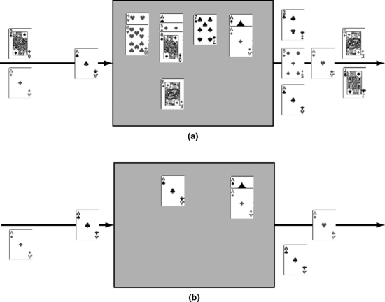
FIGURE 3.5 Illustration of Little’s law to compute AVF. (a) Flow of ACE and un-ACE instructions through a hardware structure, such as an instruction queue. (b) Flow of only ACE instructions through the structure.
This is a powerful equation that not only allows one to quickly do back-of-the-envelope calculations of AVF but also provides insight into the parameters AVF depends on.
To quickly compute the approximate AVF of a 32-entry instruction queue, let us categorize instructions into ACE and un-ACE and ignore the ACE bits in un-ACE instructions. Assume that the instruction per cycle (IPC) of ACE instructions is two and average delay of an instruction in the instruction queue is five cycles. What is the approximate AVF of the instruction queue?
SOLUTION BACE = 2 IPCs, LACE=5 cycles. Then, AVF=2×5/32=10/32=31%.
Compute the AVF of a branch commit table in a microprocessor. At the decode stage, every decoded branch and its associated information are entered into the branch commit table. When the branch commits and is deemed to have been mispredicted, then the information in the commit table is accessed to recover the state of the pipeline and restart the pipeline from the correct-path instruction after the branch. Assume an entire entry in the branch commit table is either ACE or un-ACE, the average IPC of the machine is two, the decode to commit delay (including queueing delay) is 30 cycles, one out of five instructions are branches, the branch misprediction rate is 3%, and the branch commit table has 64 entries.
SOLUTION At any instant, there are four types of entries in the branch commit table: ACE mispredicted branch entries that will be used for recovery, un-ACE branch instructions that are predicted correctly, wrong-path un-ACE branch entries, and idle un-ACE entries. There is one branch per five committed instructions. The branch misprediction rate is 3% so 3 out of 100 branches are mispredicted. In other words, 3 out of 500 instructions are mispredicted. The mispredicted branch IPC is then 2 × (3/500) = 0.012. Since the decode to commit delay (including queueing delay) is 30 cycles, the average number of mispredicted branch instructions in the commit table is 0.12 × 30 = 0.36. The total number of entries in the commit table is 64. Hence, the AVF = 0.36/64 = 0.56%.
Although Little’s law is useful to compute the AVF of hardware structures, it must be applied carefully. Little’s law cannot be applied if the ACE objects flowing through a structure change. For example, Little’s law cannot be directly applied to an adder, which takes two operands as inputs and produces one output. In this case, Little’s law can be applied separately to the input and output datapath latches.
3.9.1 Implications of Little’s Law for AVF Computation
Using Little’s law to compute the AVF gives one four important insights into the computation of AVF and the factors AVF depends on. First, AVF is a function of the architecturally sensitive area of exposure to radiation. This is expressed through Little’s law by multiplying the number of incoming ACE bits into a structure with the delay experienced in the structure. “Sensitive” area in this context refers to the fraction of area that on average is occupied by ACE objects.
Second, IPC alone may not determine the AVF of microprocessor pipeline structures. Let us consider the instruction queue in a processor pipeline. Let us define ACE IPC and ACE latency as the IPC of ACE instructions and latency of ACE instructions through the instruction queue, respectively. The instruction queue usually has the same IPC as the retire unit in a processor pipeline. A benchmark with high IPC can have high ACE IPC but low ACE latency because instructions may be flowing rapidly through the pipeline. Similarly, a benchmark with low IPC can have low ACE IPC, but instructions may be stalled behind cache misses, making ACE latency high. Consequently, both these benchmarks can have very similar AVF for the instruction queue in the pipeline.
Third, it is often not unusual to assume that a structure’s AVF decreases if objects move faster through the structure, thereby reducing the exposure time to radiation. However, the AVF may not actually decrease if there is a corresponding increase in the bandwidth of ACE objects flowing into the structure.
Fourth, one can relate AVF of different structures using Little’s law. If objects flow from a structure A to a structure B, then in the steady state, the average bandwidth of ACE objects through both A and B will usually be the same. To compute the AVF, however, one needs the average delay through objects A and B and the size of each structure, which may differ. However, in the degenerate case where a sequence of single-bit storage cells with unit delay is connected (e.g., sequence of flow-through latches in a datapath), the AVF of each of these storage cells is the same.
3.10 Computing AVF with a Performance Model
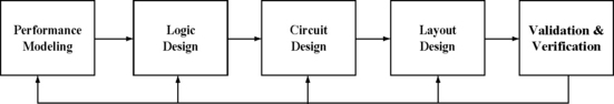
To study the trade-off between performance, power, and soft errors, and to design the appropriate machine, architects need an early AVF estimate for the chip they are designing. Figure 3.6 shows the different steps in the design of a high-performance microprocessor. Typically, this process starts with a performance model—typically written in C or C++. A performance model is an abstract representation of the machine’s timing behavior, which allows architects to predict the performance of the machine under design. This is followed by the actual architectural definition and logic design of the processor. This is often done in a Register Transfer Language (RTL), such as Verilog. Once the RTL is ready, circuit designers convert the logic blocks into circuit blocks using a variety of tools. This is followed by layout design, validation, and verification. The outputs from the validation and verification steps are fed back to the different stages of the design to fix bugs. High-performance chipsets usually follow the same flow. Nevertheless, some application-specific integrated circuits may skip some of the intermediate steps (e.g., they may need to model the performance of the chip).
The two obvious places to model the AVF are in the performance model and in the RTL model. The advantage of the RTL model is that it has the detailed state of microprocessor or chipset structures. Hence, one could use statistical fault injection into different RTL states (e.g., latches) and see if the fault shows up as a user-visible error and thereby compute the AVF. Chapter 4 discusses in detail the advantages and drawbacks of statistical fault injection. AVF evaluation with an RTL model, however, poses two problems for an architect. First, RTL may not be available long after the architecture specification has been defined. By the time RTL is created and the architects find out what the AVFs are, it may be too late to do any major changes to the design because of schedule pressures. It may, however, be possible to use an earlier version of the RTL (from a previous generation chip), but that may still be error prone.
Second, RTL simulations are orders of magnitude slower than performance models. RTL simulations can often only be realistically run for tens of thousands of instructions, but the effect of a fault in a microarchitectural structure may not show up till after tens of millions of instructions. Further, since soft errors are an average and statistical quantity, it is critical to do such simulations over a number of benchmarks, potentially spanning millions to billions of instructions. Further, statistical fault injection into a chip with billions of transistors necessitates an explosive number of simulations to reach a statistical significance.
Nevertheless, for many structures, such as flow-through pipeline latches, the fault-to-error latency is fairly small (e.g., less than 1000 cycles often). Furthermore, some of these structures may not be available in the performance model. For such structures, statistical fault injection into the RTL is a desirable way to measure the AVF. The section Computing AVFs Using Statistical Fault Injection into RTL, p. 146, Chapter 4, discusses these issues in greater detail.
3.10.1 Limitations of AVF Analysis with Performance Models
The AVF analysis technique using a performance model can provide early estimates of per-structure AVFs, but it also has four limitations that readers should be aware of.
What Is the Scope?
As discussed in Chapter 1 (see Faults, p. 6), the concept of MTTF is fundamentally tied to a “scope.” A scope is a domain with which an MTTF value is associated. Because MTTF is inversely proportional to the FIT rate and hence to the AVF, the concept of AVF is also related to the scope for which the AVF is defined. For example, if the scope is defined to be the full system, including I/O devices, then an object is ACE only if its effect shows up at the I/O interface. In contrast, if the scope is defined to be at the cache-to-main memory interface, then one can declare an object arriving at the cache-to-memory interface to be ACE if it shows up at this interface. But what is an ACE bit at the cache-to-memory interface may be un-ACE when the scope is expanded to the full system (e.g., a memory value with an error may never be written back to disk).
Further, the scope at which an error shows up depends on the user’s interaction with a program. Normally, a program’s outputs are just the values sent by the program via I/O operations. However, if a program is run under a debugger, then the program variables examined via the debugger become outputs and influence the determination of the ACE bits.
For AVF analysis in a performance model, one usually requires a precise definition of what constitutes the scope. It is assumed that the scope extends to an I/O device. In practice, it is hard to track values this far. However, performance models can track values well beyond the point that they are committed to architectural registers or stored to memory to determine whether they could potentially influence the output. Given such a definition of a scope, one can determine in a performance model the ACE and un-ACE bits.
What Is a Correct Output?
Besides the scope, one also needs a precise definition of what constitutes the correct output. This does not necessarily correspond to meeting the precise semantics of the architecture, which can allow multiple correct outputs for the same program. Similarly, in a multiprocessor system, multiple executions of the same parallel program may yield different outcomes due to race conditions. Whether a bit is ACE or un-ACE may depend on the outcome of a race.
To make the methodology precise, ACE analysis computes the AVF for a specific dynamic instance or execution of a program. Given a specific execution of a program, the ACE analysis assumes that the final system output is the correct one. Any bit flip that would have caused the program to generate an output different from the expected system output for that instance constitutes an error. In a multiprocessor system, ACE analysis would use the outcome of the race in the particular execution under study to determine the ACE and un-ACE.
Thus, this style of AVF estimation is a postanalysis method. That is, one runs the programs, collects statistics, and analyzes what the per-structure AVFs would have been. This is, however, not different from how performance simulators estimate performance and power.
ACE Analysis Provides an Upper Bound
As may be obvious by now, proving that a bit is un-ACE is easier than proving that the bit is ACE. For example, if one has two consecutive stores to the same register A without any intervening read, then register A’s bits are dynamically dead and hence un-ACE in the interval from the first store to the second store. However, this second store may not occur within the window of simulation or the first store may have been evicted from the AVF analysis window, in which case one cannot determine if register A’s bits were ACE or un-ACE, unless the program can be run to completion.
Nevertheless, since a conservative (upper bound) SER and hence AVF estimate are desired, the analysis first assumes that all bits are ACE bits unless it can be shown otherwise. Then it identifies as many sources of un-ACE bits as it can. The analysis does not need (nor claims) to have a complete categorization of un-ACE bits; however, the more comprehensive the analysis is, the tighter the bound will be.
Recently, a couple of studies have examined the preciseness with which AVFs can be computed. Wang et al. [14] computed AVFs using ACE analysis on a relatively less detailed performance model and found that the resulting AVF is two to three times higher than what SFI would predict from an RTL model. The authors argued that this is because it is difficult to add the necessary detail to a performance model to compute the appropriate AVFs. Biswas et al. [1] have shown, however, that such details are not hard to add to a performance simulation model to appropriately compute precise AVFs.
Similarly, Li et al. [8] argue that AVF analysis reaches its limit when one considers tens of thousands of computers or a very high intrinsic FIT rate (significantly higher than what a radiation-induced transient fault would cause). It is unclear what underlying phenomenon is forcing this limit. One possibility is that higher numbers of computers or higher intrinsic FIT rate may be introducing multi-bit faults. In such as case, the basic AVF analysis needs to be extended and the error rate computed differently. For an example of how to compute the SER from double bit errors, the reader is referred to the scrubbing analysis in Chapter 5.
The reader should also note that often a conservative upper bound on AVF is sufficient for what a designer is looking for. If the conservative upper-bound AVF estimates satisfy the soft error budget of a chip, then the designer may not care to further refine them. If not, the designers may continue to refine the AVF analysis for the most vulnerable structures until they are satisfied with the analysis.
Chapter 4 shows how one could extend this analysis to gather best estimate AVF numbers based on the properties of certain structures.
ACE Analysis Approximates Program Behavior in the Presence of Faults
One subtle issue that may not be immediately obvious is that ACE analysis attempts to approximate the behavior of a faulty instance of a program from an analysis of a fault-free execution of the same program. For example, Figure 3.7b shows the dynamic execution of a program in which the program takes the wrong branch direction because of a fault. Currently, ACE analysis assumes that any such control flow inducing instruction is ACE. Nevertheless, it is possible that even if the branch takes the incorrect path, it will eventually produce the correct result, thereby making the result of some branches un-ACE [13]. Such branches are called Y-branches. The impact of this phenomenon is expected to be limited. Nevertheless, this is yet another place where ACE analysis provides an upper-bound estimate. One way to make the analysis more precise for Y-branches is to simulate both paths of a branch during a program’s execution and determine if the paths eventually converge with the same architectural state.

FIGURE 3.7 Examples of fault-free (a) and faulty (b) flows of a program execution. ACE analysis attempts to approximate the behavior of (b) using (a).
CAM structures introduce a similar challenge. Chapter 4 shows how to compute the AVF of such CAM structures.
3.11 ACE Analysis Using the Point-of-Strike Fault Model
As it was discussed earlier, one can use the following equation—based directly on the point-of-strike fault model—to compute the per-structure AVFs:

Thus, the following three terms are needed:
![]() sum of residence cycles of all ACE bits of objects resident in the structure during program execution
sum of residence cycles of all ACE bits of objects resident in the structure during program execution
![]() total execution cycles for which the ACE bits’ residence time is observed
total execution cycles for which the ACE bits’ residence time is observed
Using a performance model, one can compute all the above. This chapter illustrates this technique using objects that carry instruction information along the pipeline (Figure 3.8). Chapter 4 discusses advanced techniques to compute AVF for structures that carry other types of objects, such as cache blocks.

The AVF algorithm can be divided into three parts. As an instruction flows through different structures in the pipeline, the residence time of the instruction in the structure is recorded. Then, before the instruction disappears from the machine, either via a commit or via a squash, the structures through which it flowed are updated with a variety of information, such as the residence cycles, whether the instruction committed, etc. (part 1). Also, if the instruction commits, the instruction is put in a postcommit analysis window to determine if the instruction is dynamically dead or if there are any bits that are logically masked (part 2). Finally, at the end of the simulation, using the information captured in parts 1 and 2, one can easily compute the AVF of a structure (part 3).
To compute whether an instruction is an FDD or a TDD instruction and whether any of the result bits has logical masking, one must know about the future use of an instruction’s result. The analysis window is used to capture this future use. When an instruction commits, it is entered into the analysis window, linking it with the instructions that produced its operands. At any time, one can analyze the future use of an instruction’s results by examining its successors in the analysis window. Of course, because the analysis window must be finite in size, one cannot always determine the future use precisely. An analysis window of a few thousand instructions usually covers most of the needed the future use information, but practitioners have used tens of thousands of instructions for this window.
The analysis window needs three subwindows that compute FDD, TDD, and logical masking information. Each subwindow can be implemented with two primary data structures: a linked list of instructions in commit order and a table indexed via architectural register number or memory address. The linked list maintains the relative age information necessary to compute future use. Each entry in the table maintains the list of producers and consumers for that register or memory location. The FDD, TDD, and logical masking information can all be computed using this list of producers and consumers. Thus, a list with two consecutive producers for a register R and no intervening consumer for the same register R can be used to mark the first producer of R as a dynamically dead instruction.
3.11.1 AVF Results from an Itanium®2 Performance Model
This section presents a case study of AVF evaluations for two structures: an instruction queue and execution units for an Itanium® 2 processor pipeline. This case study is based on the evaluations presented by Mukherjee et al. [10]. The evaluation methodology will be discussed first followed by AVF analyses for an instruction queue and latches in input and output datapaths in execution units. This case study demonstrates how ACE analysis can compute both SDC and DUE AVFs.
Evaluation Methodology
The evaluation uses an Itanium® 2-like IA64 processor scaled to 2003 technology. Itanium®2 is one of Intel® Corporation’s high-end processor architectures. This processor was modeled in detail in the Asim performance model framework [5] developed by a group in the Compaq Computer Corporation and was eventually licensed and developed further by architects in Intel Corporation. In Asim, Red Hat Linux 7.2 was modeled in detail via an OS simulation front end. For wrong paths, the simulator fetched the misspeculated instructions but did not have the correct memory addresses that a load or a store may have accessed. This processor model is augmented with an instrumentation to evaluate per-structure AVFs.
Figure 3.9 lists the skip intervals and input set selected for each of the SPEC 2000 programs used for this analysis. Because it is difficult, if not impossible, to simulate in detail an entire program, simulation models typically simulate only sections of programs or benchmarks to predict performance. The skip intervals shown here were computed using simpoint analysis of Sherwood et al. [12] modified for the IA64 ISA [11]. The numbers presented here are only for the first simpoint. Simpoints provide sections of the program that can best predict the performance of the whole program itself. Although simpoints do not necessarily provide sections that can best predict AVFs, it is probably a fair approximation for the AVFs as well. In this evaluation, each simpoint is simulated for 100 million instructions (including NOPs). The benchmarks were compiled with the Intel® electron compiler (version 7.0) with the highest level of optimization.
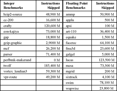
FIGURE 3.9 Benchmarks used for AVF studies of the instruction queue and execution unit of the Itanium®2 pipeline under study. M = million. Reprinted with permission from Mukherjee et al. [10]. Copyright ©2003 IEEE.
Program-Level Decomposition
Figure 3.10 shows a decomposition of the dynamic stream of instructions based on whether the instruction’s output affects the final output of the benchmark. An instruction whose result may affect the output is an ACE instruction, while an instruction that definitely does not affect the final output is un-ACE. As the figure shows, on average, about 46% of the instructions are ACE instructions. The rest are un-ACE instructions. Some of these un-ACE instructions still contain ACE bits, such as the opcode bits of prefetch instructions. Because this analysis is conservative, there may be other opportunities to move instructions from the ACE to un-ACE category.

FIGURE 3.10 ACE and un-ACE breakdown of the committed instruction stream in an Itanium®2 pipeline for the benchmarks shown in Figure 3.9.
NOPs, predicated false instructions, and performance-enhancing prefetch instructions account for 26%, 7%, and 1%, respectively. NOPs are introduced in the IA64 instruction stream to align instructions on three-instruction bundle boundaries. These NOPs are carried through the Itanium® 2 pipeline. Finally, dynamically dead instructions account for 20% of the total number of committed instructions.
AVF Analysis for the Itanium®2 Instruction Queue
Figure 3.10 shows the fraction of cycles a storage cell in the instruction queue contains ACE and un-ACE bits. An instruction queue is a structure into which the processor fetches instructions. A separate scheduler usually identifies and dispatches from this queue instructions that are ready to be executed. This calculation assumes each entry of the instruction queue is approximately 100 bits. An IA64 instruction is 41 bits, but the number of bits required in the entry is higher because a large number of bits are required to capture the in-flight state of an instruction in the machine. Out of these 100 bits, five bits are control bits and cannot be derated. Of the remaining 95 bits, seven opcode bits are not derated (i.e., considered ACE) for any instruction. Additionally, the six predicate specifier bits of falsely predicated instructions or the seven destination register specifier bits for FDD and TDD instructions are not derated.
Figure 3.11a shows that on average, a storage cell in the instruction queue contains an ACE bit about 29% of the time. Thus, the AVF of the instruction queue is 29%. On average, a cell is idle 38% of the cycles and contains a nonidle un-ACE bit about 33% of the cycles. This 33% includes 6% uncommitted, such as wrong-path instructions, 16% neutral, such as NOPs, and 11% dynamically dead. Across the simulated portions of the benchmark suite (Figure 3.12), the AVF number ranges between 14% and 47% for the instruction queue. The floating-point programs, in general, have higher AVFs than to integer programs (31% vs. 25%, respectively). This is because floating-point programs usually have many long-latency instructions and few branch mispredictions.

FIGURE 3.11 ACE and un-ACE breakdown of an instruction queue in an Itanium®2 pipeline. (a) The SDC AVF for the unprotected instruction queue is 29%. (b) The DUE AVF of the same instruction queue with parity protection, but no recovery, is 62% (29% true DUE AVF + 33% false DUE AVF).
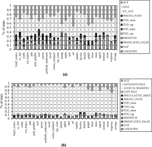
FIGURE 3.12 ACE and un-ACE breakdown for an instruction queue (a) and execution unit (b) for an Itanium®2 pipeline. Reprinted with permission from Mukherjee et al. [10]. Copyright ©2003 IEEE.
Figure 3.11b shows the false DUE AVF of the instruction queue, assuming that it is protected with parity. The parity bit is checked when an instruction is ready for issue. The entire nonidle un-ACE portion is now ascribed to the false DUE AVF. Hence, the false DUE AVF of the instruction queue protected with parity is 33%. The total DUE AVF is 29% + 33% = 62%.
Figure 3.13 shows how to approximate AVFs (at the instruction level) for the instruction queue using Little’s law. The AVF of the instruction queue can be approximated as the ratio of the average number of ACE instructions in the instruction queue to the total number of instruction entries in the instruction queue, which is 64 in the machine simulated. The number of ACE instructions in the instruction queue in an average cycle, as given by Little’s law, is the product of the bandwidth (ACE IPC) and the average number of cycles an instruction in the instruction queue can be considered to be in ACE state (ACE latency). It should be noted that an instruction can persist even after it is issued for the last time. Thus, after an ACE instruction is issued for the last time, the ACE bits holding the ACE instruction become un-ACE. The ACE IPC and ACE latency were obtained from the performance model.

FIGURE 3.13 AVF breakdown for an instruction queue with Little’s law. Number of ACE instructions = ACE IPC × ACE latency. AVF = number of ACE instructions/number of instruction queue entries. Reprinted with permission from Mukherjee et al. [10]. Copyright ©2003 IEEE.
Using the ACE IPC and ACE latency, the AVFs in Figure 3.13 can be computed. This method computes an average AVF of 19%, which is 10% lower than that of actual AVF for the instruction queue reported earlier. This difference can be attributed to the ACE bits of un-ACE instructions, such as prefetch and dynamically dead instructions, whose results do not affect the final output of a program. Figure 3.13 accounts for these as un-ACE bits, but ACE numbers in Figure 3.11 and Figure 3.12 include them. If the Little’s law analysis was done at the bit level, instead of instruction level as in Table 2, then the average AVF of 29% in Figure 3.11 would have matched.
Figure 3.13 also explains why lucas has an AVF similar to ammp although lucas has one of the highest ACE IPCs. This is because the AVF depends on both the ACE IPC and ACE latency. Although lucas has a high ACE IPC, it has relatively low ACE latency. Consequently, the product of these two terms results in an AVF similar to ammp’s, which has a low ACE IPC but a high ACE latency.
AVF for Execution Units
This section describes the AVF numbers of the execution units in the simulated machine model. In this six-issue machine, there are four integer pipes and two floating-point pipes. Integer multiplication is, however, processed in the floating-point pipeline. When integer programs execute the floating-point pipes lie idle. It is also assumed that the execution units overall have about 50% control latches and 50% datapath latches. First, how to derate the entire execution unit is discussed so that the results would apply to both the control and the datapath latches. Then, it will be shown how to further derate the datapath latches.
Figure 3.12b shows that the execution units on average spend 11% of the cycles processing ACE instructions (with a range of 4% to 27%). Thus, the average AVF of a latch in the execution units is 11%. Interestingly, the execution units’ AVF is significantly lower than that of the instruction queue. This is due to three effects. First, the instruction queue must hold the state of the instructions until they execute and retire. Thus, ACE instructions persist longer in the instruction queue than the time they take to execute in the execution units.
Second, speculatively issued instructions succeeding cache miss loads must replay through the instruction queue. However, only the last pass through the execution units matters for correct execution. The execution unit state for all prior executions is counted as un-ACE. It should be noted that this is possible in this processor model because a corrupted bit in one of the instructions designated for a replay does not affect the decision to replay. The information necessary to make this decision resides elsewhere in the instruction queue.
Third, the floating-point pipes are mostly idle while executing integer code, greatly reducing their AVFs.
This analysis computes a single AVF for both the control and the datapath latches in the execution units. However, the datapath latches can be further derated based on whether specific datapath bits are logically masked or are simply idle. Here logical masking is applied to data values (and hence datapaths) only; analyzing logical masking for control latches would be a complex task.
Logical masking functions were implemented only for a small but important subset of the roughly 2000 static internal instruction types in the processor model. This subset contains a variety of functions, including logical OR, AND. It was also estimated that another 20% of the instructions (including loads, stores, and branches) will not have any direct logical masking effect. The combination of these two categories covers the vast majority of dynamically executed instructions. Figure 3.12b shows that this logical masking analysis further reduces the AVF by 0.5% (averaged across both control and data latches, although this does not apply to control latches). It is expected that the incremental decrease in AVF due to the remaining unanalyzed instruction types will be small. Transitive logical masking, which would further reduce the AVF number for the datapath latches, was not considered in this analysis.
Datapath latches can be further derated by identifying the fraction of time they remain idle. For example, an IA64 compare instruction produces two predicate values—a predicate value and its complement. However, in the simulated implementation, these two result bits are sent over a 64-bit result bus, leaving 62 of the datapath lanes idle. This effect further reduces the AVF by 1.5%, as shown by DATAPATH_IDLE in Figure 3.12b Depending on the implementation, however, the DATATPATH_IDLE portion can also be viewed as bits that get logically masked at the implementation level. In contrast, UNIT_IDLE in Figure 3.12b refers to the whole execution unit being idle because of the lack of any instruction issued to that unit.
Overall, the average AVF for the execution units is reduced to 9% when logical masking and idle latches are accounted for. Across the simulated portions of our benchmark suite, the AVF for the execution units ranges from 4% to 27%.
It should be noted that Little’s law cannot be applied to the entire execution units because the objects flowing through the execution units change. Nevertheless, Little’s law can be applied to the input and output datapath latches.
3.12 ACE Analysis Using the Propagated Fault Model
Li et al. [9] developed a tool called SoftArch, which makes use of the propagated fault model in a performance simulator to compute the SER. Instead of computing the AVFs directly using the equations shown earlier (see AVF Equations for a Hardware Structure, p. 96), SoftArch evaluates the AVF indirectly by evaluating the derated and nonderated MTTF for a particular structure. The AVF can be obtained by dividing the nonderated MTTF by the derated MTTF. The reader should note that computing AVFs using either the point-of-strike model directly or the propagated fault model indirectly (like SoftArch does) suffers from the same limitations outlined in Limitations of AVF Analysis with Performance Models (p. 103).
Figure 3.14 shows a hypothetical example of how to compute the MTTF using the propagated fault model. Each of the four faults shown in the figure has a certain probability of occurrence and a corresponding nonderated error rate. The second fault gets masked, but the TTF for the first, third, and fourth errors are 1000, 10000, and 20000, respectively. If one assumes that these three errors are completely independent of each other and occur with equal probability (=1/3), then the MTTF would be [1000 × (1/3) + 10000 × (1/3) + 20000 × (1/3)] = 10230 cycles. In reality, however, a program may run for longer than 20000 cycles. One cannot assume that the distribution of errors is uniform, although the underlying faults from alpha particle or neutron strikes may occur uniformly.

FIGURE 3.14 Hypothetical example showing different TTFs. The first timeline shows the occurrence of four potential faults. Each has a certain probability of occurrence. Some of these will get masked. The second timeline shows when the faults show up as a user-visible error at some output.
To illustrate how SoftArch computes the MTTF, let us consider the following example. Let us assume that
![]() a chip has only one unit in which the probability of an intrinsic fault (p) is 0.1 in each cycle
a chip has only one unit in which the probability of an intrinsic fault (p) is 0.1 in each cycle
![]() the workload is an infinite loop
the workload is an infinite loop
![]() each iteration in the loop has four cycles
each iteration in the loop has four cycles
![]() the unit always has ACE values in the first two cycles of the loop and un-ACE values in the last two cycles of the same loop
the unit always has ACE values in the first two cycles of the loop and un-ACE values in the last two cycles of the same loop
![]() the program is fail-stop with respect to this unit, that is, as soon as an error is detected, the program stops
the program is fail-stop with respect to this unit, that is, as soon as an error is detected, the program stops
![]() T is a random variable that designates the TTF, T can assume the values 1, 2, 5, 6, 9, 10, …, T cannot be 3, 4, 7, or 8 because the unit has un-ACE values in the last two cycles of the loop and the MTTF is the expected value of T or E(T).
T is a random variable that designates the TTF, T can assume the values 1, 2, 5, 6, 9, 10, …, T cannot be 3, 4, 7, or 8 because the unit has un-ACE values in the last two cycles of the loop and the MTTF is the expected value of T or E(T).
Then, E(T) = 1 × p + 2 × (1 – p) × p + 3 × 0 + 4 × 0 + 5 × (1 – p)2 × p + … This is an infinite series. For this particular example, it sums to 18.53 cycles. For such a loop, Li et al. have created a closed form of the equation as
where LT is number of cycles in the loop. Using LT = 4, p = 0.1, we get MTTF=18.53 cycles as well.
The above example shows how to compute the MTTF when there is only one unit in a chip. To compute the MTTF in the presence of multiple units across a chip, SoftArch must keep track of how faults propagate through the units during a program’s execution. Figure 3.15 shows such an example of fault propagation. Let us assume v6 = NOT (v4), v4 = v1 + v2, v5 = v2 + v3, and f1, f2, and f3 are the faults generated in v1, v2, and v3, respectively, and v6 is an output of the computation. It should be noted that v5 is dynamically dead. In this case, only faults f1 and f2 affect whether output v6 has an error. Hence, v1, v2, v4, and v6 constitute the ACE path. SoftArch tracks propagation of such ACE values through the dataflow graph of the program to compute the probability of an error in an outcome.

Then, the MTTF of an indefinitely executing program can be expressed as

where ti is the time when fault i manifests itself as an error in the output and Prob(vi) is the probability that the value vi corresponding to the fault i has an error, but no prior value v1, v2, …, vi–1, has an error. As may be obvious, v1, v2, …, vN constitute an ordered set of values, errors in which show up at t1, t2, …, tN times, where t1 <t2 … <tN. SoftArch computes the MTTF by keeping track of the vis, fis, and tis. For finite programs, SoftArch proposes to run the same program repeatedly (and therefore indefinitely) and, thereby, compute the MTTF.
Figure 3.16 shows SoftArch’s evaluation of AVFs for several processor structures. As described earlier, the AVF for a processor structure can be evaluated as the ratio of the nonderated and derated MTTF for that particular structure. For this evaluation, SoftArch makes the simplifying assumption that any value stored to memory is an output. Nevertheless, this methodology still provides an upper-bound estimate of what the AVF is. Figure 3.16 shows that the AVFs vary from 0% to 49% for different structures and benchmarks.
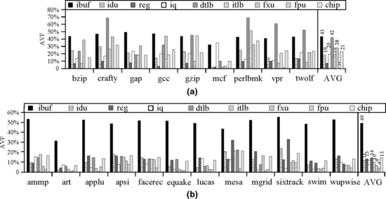
FIGURE 3.16 AVFs from SoftArch’s evaluation of a processor roughly resembling IBM’s Power4 architecture. (a) AVF for SPECint 2000. (b) AVF for SPECfp 2000. Reprinted with permission from Li et al. [9]. ibuf = instruction buffer, idu = instruction decode unit, reg = architectural register file, iq = instruction queue, dtlb = data TLB, itlb = instruction TLB, fxu = fixed point (integer) execution unit, fpu = floating point unit, and chip = entire chip. Copyright ©2005 IEEE.
Unlike ACE analysis that directly computes the AVF, SoftArch first computes the MTTF and then derives the AVFs from them. Theoretically, both are valid methods to compute AVFs. Both suffer from the same disadvantages arising out of using a performance model to compute the AVFs. Both may require significant amounts of memory in the software used to compute the AVFs. ACE analysis may require a significant amount of memory to keep track of dynamically dead instructions. This method attempts to limit the amount of memory needed by using a smaller window of analysis to track dynamically dead instructions, thereby incurring some inaccuracy. SoftArch may require a significant amount of memory to track propagation of ACE values through the dataflow graph. SoftArch reduces this memory requirement by tracking values only through registers but not through memory of the simulated benchmarks, which would also incur some inaccuracy. A systematic evaluation of the merits and demerits of each method, however, is a topic of future work.
3.13 Summary
AVF identifies the fraction of faults that result in a user-visible error for a transistor, bit, or structure. The circuit-level error rate needs to be derated (or multiplied) by the AVF to obtain the overall SER for the component in question. AVFs can vary widely—from 0% to 100%. To reduce the overall SER of the chip under design, designers can choose structures with relatively high bit count and high AVF as candidates for protection.
The SDC FIT of a bit can be expressed as the product of its SDC AVF and circuit-level SER. Similarly, the DUE FIT of a bit can be expressed as the product of its DUE AVF and circuit-level SER. The DUE AVF of a bit is the sum of the true and false DUE AVFs. The true DUE AVF of a bit is its SDC AVF without any error detection. The SDC FIT of a chip can be computed by summing the SDC FIT of all of its constituent transistors, bits, or structures. The same can be done for the DUE FIT.
This formulation of FIT rates and AVFs applies to a single-bit fault model, which is the dominant component of radiation-induced soft errors. Multibit faults can also be analyzed and their formulation will be discussed later in this book. It is also important to note that the AVF is assigned to the bit that was struck by an alpha particle or a neutron and not to a bit where the fault may have propagated.
AVFs can be computed based on ACE principles. A bit is ACE if it needs to be correct for the correct execution of a program. Otherwise, it is un-ACE. The fraction of cycles for which a bit is ACE is its AVF. A structure’s AVF is the average AVF of all its constituent bits. Alternatively, a structures’s AVF can be expressed as the ratio of the average number of ACE bits in a cycle and the total number of bits in the structure.
Often it is easy to identify the source of un-ACEness and hence AVF can be conservatively computed by analyzing the un-ACE bits during a program’s execution. Un-ACE bits can arise from both microarchitectural and architectural components. Examples of microarchitectural un-ACE bits are bits that are idle, bits containing misspeculated states. Examples of architectural un-ACE bits are nonopcode bits of a NOP instruction, nonopcode bits of prefetch and branch hint instructions, and nonopcode and nonregister specifier bits of dynamically dead instructions. Using such an analysis, the AVFs of different structures can be computed using a performance simulation model.
3.14 Historical Anecdote
Prior to the introduction of the term AVF, Intel had widely used the term “logic derating factor” to indicate the same. In 2001, we, a group of four engineers, tried to develop the AVF methodology and frequently talked about cross-purposes because of the term “derating factor.” The reason is because the two terms—“derating” and “derating factor”–go in different directions. When we reduce the derating, we increase the vulnerability of a bit to soft errors. However, when we reduce the derating factor, we reduce the vulnerability of the bit to soft errors. Quite often we would say one thing (e.g., this technique will reduce the derating) when we meant the other (e.g., this technique will reduce the derating factor). To avoid this confusion, we coined the term “vulnerability factor” to replace “derating factor.” If you derate more, we increase both the vulnerability and vulnerability factor. Since then, discussions on AVF were more meaningful than in the early days of development of the AVF ideas. Currently, the term AVF is widely used across Intel’s soft error groups and management circles.
References
Biswas A., Racunas P., Emer J., Mukherjee S.S. Computing Accurate AVFs using ACE Analysis on Performance Models: A Rebuttal. Computer Architecture Letters (CAL). December 2007.
Butts J.A., Sohi G. Dynamic Dead-Instruction Detection and Elimination. 10th International Conference on Architectural Support for Programming Languages and Operating Systems (ASPLOS). October 2002:199–210.
Fahs B., Bose S., Crum M., Slechta B., Spadini F., Tung T., Patel S.J., Lumetta S.S. Performance Characterization of a Hardware Mechanism for Dynamic Optimization. 34th Annual International Symposium on Microarchitecture (MICRO). December 2001:16–27.
Choi Y., Knies A., Gerke L., Ngai T.-F. The Impact of If-Conversion and Branch Prediction on Program Execution on the Intel Itanium Processor. 34th Annual International Symposium on Microarchitecture (MICRO). December 2001:182–191.
Emer J., Ahuja P., Binkert N., Borch E., Espasa R., Juan T., Klauser A., Luk C.K., Manne S., Mukherjee S.S., Patil H., Wallace S. Asim: A Performance Model Framework. IEEE Computer. February 2002;Vol. 35(No. 2):68–76.
Hennessy J.L., Patterson D.A. Computer Architecture: A Quantitative Approach. Elsevier Science, 2003.
Lazowska E.D., Zahorjan J., Graham G.S., Sevcik K.C. Quantitative System Performance. Englewood Cliffs, New Jersey: Prentice-Hall, 1984.
Li X., Adve S.V., Bose P., Rivers J.A. Architecture-Level Soft Error Analysis: Examining the Limits of Common Assumptions. International Conference on Dependable Systems and Networks (DSN). 2007:266–275.
Li X, Adve S.V., Bose P., Rivers J.A. SoftArch: An Architecture-Level Tool for Modeling and Analyzing Soft Errors. International Conference on Dependable Systems and Networks (DSN). 2005:496–505.
Mukherjee S.S., Weaver C.T., Emer J., Reinhardt S.K., Austin T. A Systematic Methodology to Compute the Architectural Vulnerability Factors for a High-Performance Microprocessor. 36th Annual International Symposium on Microarchitecture (MICRO). December 2003:29–40.
Patil H., Cohn R., Charney M., Kapoor R., Sun A., Karnunanidhi A. Pinpointing Representative Portions of Large Intel Itanium Programs with Dynamic Instrumentation. 37th Annual International Symposium on Microarchitecture (MICRO). 2004:81–92.
Sherwood T., Perelman E., Hamerly G., Calder B. Automatically Characterizing Large Scale Program Behavior. 10th International Conference on Architectural Support for Programming Languages and Operating Systems (ASPLOS). October 2002:45–57.
Wang N., Fertig M., Patel S. Y-Branches: When You Come to a Fork in the Road, Take It. 12th International Conference on Parallel Architectures and Compilation Techniques (PACT). 2003:56–67.
Wang N., Mahesri A., Patel S.J. Examining ACE Analysis Reliability Estimates Using Fault-Injection. 34th International Symposium on Computer Architecture (ISCA). 2007:460–469.
Weaver C., Emer J., Mukherjee S.S., Reinhardt S.K. Techniques to Reduce the Soft Error Rate of a High-Performance Microprocessor. 31st Annual International Symposium on Computer Architecture. June 2004:264–275.