
Hardware Error Recovery
7.1 Overview
As discussed in Chapter 1, soft errors can be classified into two categories: SDC and DUE. Some of the error coding techniques, such as parity, discussed in Chapter 5 and the fault detection techniques outlined in Chapter 6 convert SDC to DUE. In some cases, these techniques may result in additional DUE rates arising from the mechanics of the fault detection technique. This chapter discusses additional hardware recovery techniques that will reduce both SDC and DUE rates arising from transient faults. The same recovery techniques may not be as useful for permanent hardware faults because fixing the permanent fault typically would involve a part replacement, which is not discussed in this chapter.
This chapter uses the term error recovery instead of fault recovery, even though the process of detecting a malfunction was referred to as fault detection. This is because a hardware fault is a physical phenomenon involving a hardware malfunction. The effect of the fault will typically propagate to a boundary of a domain where the fault will be detected by a fault detection mechanism. Once a fault is detected, it becomes an error. Thus, a recovery mechanism will typically help a system recover from an error (and not a fault).
The reader should also note that an error recovery mechanism reduces the SDC and DUE rates of the domain it is associated with. For example, a domain could simply include the microprocessor chip. Alternatively, a domain could include an entire system. (For a detailed discussion on how faults and errors relate to the domain of fault detection and error recovery, the reader is referred to the section Faults, p. 6, Chapter 1.) To characterize the SDC or DUE rate of a domain, one can compute the domain’s MTBF as the sum of its MTTF and MTTR. At the system level, one often talks about availability, which is the ratio of system uptime (MTTF) divided by total system time (MTBF). Availability is often expressed in number of 9s. For example, five 9s would mean that the system availability is 99.999%. This would mean a system downtime of 5.26 minutes per year. Similarly, six 9s would mean a system downtime of 31.56 seconds.
Recovery schemes can be broadly categorized into forward and backward recovery schemes. In forward error recovery, the system continues fault free execution from its current state even after it detects a fault. This is possible because forward recovery schemes maintain concurrent and replicated state information, which allows them to execute forward from a fault free state. In contrast, in a backward error recovery, usually the state of the machine is rewound backward to a known good state from where the machine begins execution again.
This chapter discusses various forms of forward and backward error recovery schemes. Forward recovery schemes discussed in this chapter include fail-over systems that fail over to a standby spare, DMR systems that run two copies of the same program to detect faults, TMR systems that run triplicate versions of the same program, and pair-and-spare systems that run a pair of DMR systems with one being the primary and the other secondary standby.
The design of a backward error recovery scheme depends on where the fault is detected. If a fault is detected before an instruction’s result register values are committed, for example, then the existing branch misprediction recovery mechanism can be used to recover from an error. This chapter examines backward recovery schemes in various systems: systems that detect faults before register values are committed, systems that detect faults before memory values are committed, and systems that detect faults before I/O outputs are committed.
7.2 Classification of Hardware Error Recovery Schemes
Fundamental to any error recovery mechanism is the “state” to which the system is taken when the error recovery mechanism is triggered. For example, Figure 7.1 shows state transition of a system consisting of two bits. The initial state of the system is 00. It goes through two intermediate states—01 and 10. Eventually, it reaches the state 11 when it gets a particle strike. This changes the state incorrectly to 01. If this incorrect state transition can be detected, then the error can be flagged. Also, it is assumed that the identity of the bit that was struck is unknown, so the state cannot be reconstructed. Then, to recover from the error, there are several choices that are described below.

FIGURE 7.1 State to recover to on a particle strike. The system can revert to the initial state (reboot) or the intermediate state (backward error recovery) or continue forward from its current state (forward error recovery).
7.2.1 Reboot
The system can be reverted to its initial state, and execution can be restarted. This may require rebooting a system. In Figure 7.1, this would correspond to reverting to the initial state 00. This is a valid recovery mechanism for transient faults, if the latency of reexecution is not critical. For hard errors, however, this mechanism may not work as well since on reexecution the system may get the same error again.
7.2.2 Forward Error Recovery
The second option would be to continue the system from its current state after a fault is detected. In Figure 7.1, this would correspond to the current state 11 when the fault is encountered. This style of error recovery is usually known as forward error recovery. The key in forward error recovery is to maintain redundant information that allows one to reconstruct an up-to-date error-free state. ECC is a form of forward error recovery in which the state of the bits protected by the ECC code is reconstructed, thereby allowing the system to make forward progress.
Forward error recovery of full computing systems, including logic and ALU components, however, can be much more hardware intensive since this may use redundant copies of the entire computing state. An output comparator would identify the faulty component among the redundant copies. The correct state can be copied from one of the correct components to the faulty one. Then the entire system can be restarted.
This could be possible, for example, if there are triply redundant copies of the execution system and state. Before committing any state outside the redundant copies, the copies can vote on the state. If one of them disagrees, then the other two are potentially correct. The faulty copy can be disabled, and the correct ones could proceed. For transient faults, the faulty copy can be scrubbed of any faults and reintegrated into the triply redundant system. For permanent faults, the faulty component may have to be replaced with a fault free component.
7.2.3 Backward Error Recovery
Backward error recovery is an alternate recovery scheme in which the system can be restored to and restarted from an intermediate state. For example, in Figure 7.1, the system could revert to the state 01 or 10. Backward recovery often requires less hardware than forward error recovery mechanisms. Backward error recovery does, however, require saving an intermediate state to which one can take the system back to when the fault is detected. This intermediate saved state is usually called a checkpoint. How checkpoint creation relates to fault detection, when outputs can be committed, when external inputs can be consumed, and how the granularity of fault detection relates to recovery are discussed below.
How Fault Detection Relates to Checkpoint Content
Broadly, there are three kinds of states in a computer system: architectural register files, memory, and I/O state. A checkpoint can comprise one or more of these states. Typically, in a computer system and particularly in a microprocessor, a register file is small and frequently written to. Memory is significantly bigger and committed to either when a store instruction executes and commits its value to memory or an I/O device transfers data to a pre-allocated portion of memory. Finally, the I/O state (e.g., disks) is usually the biggest state in a computer system and usually committed to less frequently than register files or main memory.
What constitutes a checkpoint in a system also depends on where the fault detection point is with respect to when these states are committed. This chapter describes four styles of backward error recovery depending on where the fault detection occurs. These include system where
Output and Input Commit Problems
A system with backward error recovery must also be careful about the output and input commit problems. A recovery scheme can only recover the state of a system within a certain boundary ora sphere of recovery. For example, assume that a sphere of recovery consists only of a processor chip where the fault detection occurs before memory or I/O is committed to. The checkpoint in such a recovery scheme may consist only of processor registers. On detecting an error, the processor reloads its entire state from the checkpoint and resumes execution.
The output commit problem arises if a system allows any output, which it cannot recover from, to exit the sphere of recovery. In the example just described, the processor cannot recover from memory writes it propagates to main memory or I/O operations it propagates to disks because the checkpoint it maintains does not comprehend memory or I/O state. Consequently, to avoid the output commit problem, this system cannot allow any corrupted store or I/O operation to exit the sphere of recovery until it has certified that all prior operations leading to the store or I/O operation are fault free.
Similarly, the input commit problem arises if a system restarts execution from a previous checkpoint but cannot replay inputs that had arrived from outside the sphere of recovery. During the course of normal operation in the example that was just described, a processor will receive inputs, such as load values from the memory system and external I/O interrupts. When the processor rolls back to a previous checkpoint and restarts execution, it must replay all these events since these events may not arrive again. How the backward recovery schemes solve the output and input commit problems is described in this chapter.
Granularity of Fault Detection
To only detect faults in a given domain and reduce the SDC rate, it is often sufficient to do output comparison at a coarser granularity. For example, to prevent corrupted data to exit a processor, one can compare selected instructions, such as stores, that update memory or I/O instructions, such as uncached loads and stores. Once one detects such a fault, one can halt the system and prevent any SDC from propagating to memory or disks. The same granularity of comparison may work for forward error recovery. In a triply redundant system, the component that produces the faulty store output can be identified by the output comparator, isolated, and then restarted using correct state from one of the other two components.
In contrast, the same granularity of fault detection may not work for backward error recovery. If a store output mismatch from two redundant copies is detected, it is not known which one is the faulty copy. Further, checkpoint may not be fault free since the checkpoint may consist of the architectural registers in a processor. A faulty instruction can update the architectural registers, but its effect may show up much later through a store at the output comparator. If the processor is rolled back to a previous architectural checkpoint, it cannot be guaranteed that the checkpoint itself is fault free (Figure 7.2). Hence, backward error recovery to reduce DUE necessitates fault detection at a finer granularity than what is simply needed to prevent SDC.
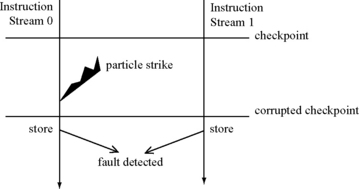
FIGURE 7.2 Granularity of fault detection in a backward error recovery executing redundant instruction streams. If only store instructions are compared, then the fault can be eventually detected. But the checkpoint prior to where the fault is detected may already have been corrupted. If the instruction stream reverts to the last checkpoint after the fault is detected, then it may not be able to correct the error.
This chapter discusses several examples of backward error recovery schemes that will highlight different aspects of the relationship between fault detection and checkpoint creation, output and input commit problems, and granularity of fault detection.
7.3 Forward Error Recovery
Forward error recovery schemes allow a system to proceed from its current state once the system detects a fault. Four styles of forward error recovery schemes are discussed in this section: fail-over systems, DMR systems, TMR systems, and pair-and-spare systems.
7.3.1 Fail-Over Systems
Fail-over systems typically consist of a mirrored pair of computing slices: a primary slice and a standby slice. The primary executes applications until it detects a fault. If the system can determine that the fault has not corrupted any architectural state, then it can copy the state of the primary slice to the standby. The standby then takes over and continues execution. This is often possible if the effect of a fault is limited to a single process. The entire system can continue execution from the point the fault is detected, but the failed process may need to restart from the beginning. The early fault-tolerant computing systems built in the 1960s and 1970s by IBM, Stratus, and Tandem were primarily fail-over systems. Marathon’s recent Endurance server used fail-over principles to recover from hardware errors (see RMT in the Marathon Endurance Server, p. 223, Chapter 6).
Figure 7.3 shows an example of an early fail-over system from Tandem Computer systems. Such a configuration had replicated processors or CPUs, power supplies, interprocessor links, etc. in each slice of the fail-over system. A bus switch monitored the primary slice for faults. If it found a fault, then it would copy the state to the standby and resume execution.

FIGURE 7.3 An example of an early fail-over, fault-tolerant computer system from Tandem [2].
Fail-over systems are often good at recovering from software bugs or system hangs but may have trouble recovering from a transient fault that corrupts the architectural state of the machine. In such cases, the standby can take over but may not be able to guarantee forward error recovery because the state of the primary slice has already been corrupted. Hence, the system will have to be rebooted, and all applications will be restarted. The next three mechanisms described in forward error recovery try to address this problem and provide better forward error recovery guarantees.
7.3.2 DMR with Recovery
DMR systems can be designed to recover from transient faults. Typically, DMR systems can detect faults using Lockstepping or RMT (see Chapter 6). An output comparator will compare the outputs of two redundantly executing instruction streams. An output mismatch will indicate the presence of a fault (Figure 7.4a). In some cases, an output mismatch can also occur due to the two slices taking correct but divergent paths. Stratus ftServer and Marathon Endurance machines both support a DMR mode with recovery.

FIGURE 7.4 Flow of operations in a DMR machine. (a) Normal operation with dual systems whose outputs are checked by an output comparator. (b) An internal error checker in System 0 fires, and the signal propagates to the output comparator. (c) The entire system is frozen. The entire system state is copied from System 1 to System 0. (d) Normal operation is resumed.
Once an output mismatch is caught, the output comparators can wait for the arrival of an internal error signal (Figure 7.4b). For example, when a bit in Slice 0 flips in a structure protected with parity, Slice 0 can propagate the parity error signal to the output comparator. Without this signal, the output comparator cannot determine the slice is in error, although it detects the existence of a fault. After determining the slice is in error, the output comparator can initiate a copy of the internal machine state from Slice 1 to Slice 0 (Figure 7.4c). This ensures that both slices have the same state. Then it can resume execution (Figure 7.4d).
Such a scheme cannot recover from all errors. How much this scheme reduces the DUE depends on how much internal error checking one has in each slice. Also, in Lockstepped DMR systems, the false DUE can be particularly high because of timing mismatches. In such a case, a recovery mechanism, such as this one, can be beneficial.
7.3.3 Triple Modular Redundancy
A TMR system provides much lower levels of DUE than a DMR system. As the name suggests, a TMR system runs three copies of the same program (Figure 7.5) and compares outputs from these programs. The fault detection technique itself could be either cycle-by-cycle Lockstepping or RMT (see Chapter 6). If the output comparison logic (often called a voter for a TMR system) determines that outputs from the three slices executing the same program redundantly are the same, then there is no fault and the output comparison succeeds.
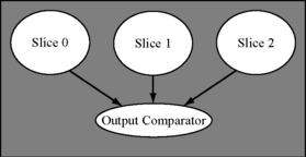
FIGURE 7.5 A TMR system. The output comparator compares outputs from three copies of the same program.
If the output comparison logic finds that only two of the three outputs match, then it will signal that the slice producing the mismatched output has experienced a fault. Typically, the TMR system will disable the slice in error but let the other two slices continue execution in a degraded DMR mode. The TMR system now has a couple of choices to bring online the slice in error. One possibility would be for the TMR system to log a service call for a technician to arrive at the site to debug the problem and restart the system.
Alternatively, it can try to fix the error and bring the slice in error into the TMR domain again. For transient faults, this would be the ideal solution. To achieve this, the degraded DMR system will be halted at an appropriate point, and the entire state of the correct slices would be copied to the one in error. Then, the TMR system can resume execution. The system will come back up automatically, but during this state copy, the entire TMR system may be unavailable to the user. This would add to the downtime of a TMR system and may reduce its availability.
The time to copy state from a correct slice of the TMR machine to the incorrect slice can be prohibitive, particularly if the TMR system copies main memory, as in Stratus’ ftServer or Hewlett-Packard’s NSAA (see Chapter 6). To reduce this time, the NSAA provides two special hooks for this reintegration. First, it provides a direct ring-based link between the memories used in the three slices of the TMR system. This allows fast copying during reintegration. Figure 7.6 shows a picture of this direct connection. The LSUs (described in Chapter 6) serve as the output comparators and input replicators for the TMR system. Memory in any slice can receive updates to it either from its local processor or from another slice coming from reintegration link.

FIGURE 7.6 Reintegration in the Hewlett-Packard NSAA design. Reprinted with permission from Bernick et al. [4]. Copyright © 2005 IEEE.
Second, the NSAA allows execution to proceed while the underlying system copies memory state from the correct to the faulty slice, thereby reducing downtime. The degraded DMR system–consisting of the correct pair of working slices—can continue to generate writes to main memory while this copy is in progress. Because the reintegration links connect to the path between the chipset and main memory, all writes to the main memory from a slice are forwarded on the reintegration links and copied to the slice being reintegrated. Eventually, the processors in the DMR system will flush their caches. Write-backs from the caches will again be forwarded to the reintegration links and copied over. Finally, the processors will be paused, and their internal state copied over to a predefined region in memory. The reintegrated processor will receive these updates and copy the state from memory to the appropriate internal registers. Thereafter, the TMR system can resume execution.
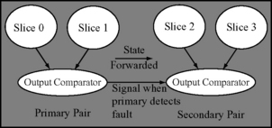
7.3.4 Pair-and-Spare
Like TMR, pair-and-spare is a classical fault-tolerance technique, which maintains a primary pair of slices and a spare pair as standby (Figure 7.7). The pairs themselves are used for fault detection with a technique such as Lockstepping or RMT. The spare pair receives continuous updates from the primary pair to ensure that the spare pair can resume execution from the point before the primary failed. This is termed forward error recovery because the spare pair does not roll back to any previous state. This saves downtime by avoiding any processor freeze to facilitate reintegration of the faulty slice. But it requires more hardware than TMR.
In the Tandem (and now Hewlett-Packard) systems, a software abstraction in its OS–called the NonStop kernel—called process pair facilitated the implementation of pair-and-spare systems [3]. A process pair refers to a pair of logically communicating processes. Each process in turn runs on a pair of redundantly executing Lockstepped processors. The process pair abstraction allows the two communicating logical processes of the pair to collectively represent a named resource, such as a processor. One process functions as the primary unit at any point in time and sends necessary state to the other logical process. If the primary process detects a fault, the spare process would take over. The NonStop kernel would transparently redirect requests to the spare without the application seeing an error. The NonStop kernel takes special care to ensure that the named resource table that provides this redirection transparency is fault free.
7.4 Backward Error Recovery with Fault Detection before Register Commit
Backward error recovery often requires less hardware than forward error recovery schemes described in the previous section. This is because in a backward error recovery, as each instruction executes, the system does not have to maintain an up-to-date fault free state. Maintaining this state—beyond what is required for fault detection only–can be quite hardware intensive (e.g., as in TMR). Instead, in a backward error recovery, the system keeps checkpoints to which it can roll back in the event of an error. A checkpoint can be more compact and less hardware intensive than maintaining a full-blown slice of the machine (e.g., as done in TMR).
This section discusses recovery and checkpointing techniques when the fault detection happens before register values are committed by a processor. Subsequent chapters examine how the sphere of recovery can be expanded by doing the fault detection before memory values or I/O values are committed. If fault detection occurs prior to committing register values, then a backward error recovery scheme can make use of the state that a modern processor already keeps to recover from a misspeculation, such as branch misprediction.
Broadly, such backward error recovery techniques can be classified into two categories: one that requires precise fault detection and one that detects faults probabilistically. Four techniques that require precise detection are discussed: Fujitsu SPARC64 V’s parity with retry, the IBM Z-series Lockstepping with retry, simultaneous and redundantly threaded processor with recovery (SRTR), and chip-level redundantly threaded processor with recovery (CRTR). For probabilistic techniques, two proposals are discussed: exposure reduction with pipeline squash and fault screening with pipeline squash and reexecution. SRTR, CRTR, and the probabilistic mechanisms are still under investigation and have not been implemented in any commercial system.
The output commit problem is solved relatively easily in these systems, but the input commit problem requires careful attention. The processor does not commit any value before the values are certified to be fault free. Hence, there is no danger of exposing a fault free state that cannot be recovered from. This solves the output commit problem. The input commit problem can arise from four sources: architectural register values, memory values, I/O devices accessed through uncached accesses (e.g., uncached loads), and external interrupts. Architectural registers are idempotent and cannot be directly changed by another processor or I/O device, so they can be reread a second time after the processor recovers. Memory values can be changed by an I/O device or by another processor, but they can be reread without loss of correctness (even if the value changes). Uncached loads must be handled carefully because an uncached load may return a value that cannot be replayed a second time. Hence, uncached loads are handled carefully by these systems. The addresses are typically compared and certified fault free before the uncached load is issued into the system. Finally, interrupts are only delivered at a committed instruction boundary, so that interrupts do not have to be replayed.
7.4.1 Fujitsu SPARC64 V: Parity with Retry
Perhaps the simplest way to implement backward error recovery is to reuse the checkpoint information that a processor already maintains. Typically, to keep a modern processor pipeline full, the processor will predict the direction a branch instruction will take before the branch is executed. For example, in Figure 7.8, the SPARC64 V processor [1] will predict the direction of the branch in the Fetch stage of the pipeline, but the actual outcome of the branch will not be known until the Execute stage.

FIGURE 7.8 Error checkers in the Fujitsu SPARC64 V pipeline. Instructions are fetched from the L1 instruction cache with the help of the branch predictor. Then they are sent to the I-Buf. Thereafter, they are decoded and sent to the reservations stations (RSA, RSE, RSF, and RSBR) for dispatch. Registers GUB, GPR, FPR, and FUB are read in the Reg-Read stage. Instructions are executed in the Execute stage. EAGA, EAGB, FXA, FXB, FPA, and FPB represent different execution units. The memory stage has a number of usual components, such as store buffer, L1 data cache, L2 cache. Reprinted with permission from Ando et al. [1]. Copyright © 2003 IEEE.
Because these branch predictions can sometimes be incorrect, these processors have the ability to discard instructions executed speculatively (in the shadow of the mispredicted branch) and restart the execution of the pipeline right after the last instruction that retired from the pipeline. To allow restart, a pipeline would checkpoint the architectural state of the pipeline every time a branch is predicted. Then, when a branch misprediction is detected, the transient microarchitectural state of the pipeline can be discarded and execution restarted from the checkpoint associated with the branch that was mispredicted. More aggressively, speculative microprocessors, such as the SPARC64 V, checkpoint the state every cycle, thereby having the ability to recover from any instruction—whether it is a branch or not.
Every time a SPARC64 V instruction is executed speculatively, its result is written to the reorder buffer for use in other instructions. The reorder buffer acts as a buffer that maintains the program order in which instructions retire, as well as the values generated speculatively by each instruction. Once an instruction retires, it is removed from the reorder buffer, and its register value is committed to the register files GPR (for integer operations) and FPR (for floating-point operations). Thus, the architecture register file automatically contains checkpointed states up to the last committed instruction. This way when a misspeculation is detected, the pipeline flushes intermediate states in the reorder buffers (as well as other more obscure states) and returns to correct state in one cycle.
The same mechanism can be used to recover from transient faults. The Fujitsu SPARC64 V processor (Figure 7.8) uses such a mechanism. It protects microarchitectural structures, address paths, and datapaths with parity codes, and ALUs and shifter with parity prediction circuits. Parity codes and parity prediction circuits can detect faults but not correct errors. When a parity error is detected, this pipeline prevents the offending instruction from retiring, throws away any transient pipeline state, and restarts execution from the instruction after the last correctly retired instruction.
7.4.2 IBM Z-Series: Lockstepping with Retry
Compared to the Fujitsu SPARC64 V, the IBM Z-series processors are more aggressive in their DUE reduction through the use of Lockstepping with retry. The Z-series processors (until the z990) implement Lockstepped pipelines that detect transient faults before any instruction’s result is committed to the architectural register file (see Lockstepping in the IBM Z-series Processors, p. 220 in Chapter 6).
The Z-series uses three copies of the register file. One copy each is associated with each of the Lockstepped pipelines. As instructions retire, speculative register state is written into these register files, so that subsequent instructions can read their source operands and make progress. The third copy is the architectural register file to which results are committed if and only if the Lockstep comparison indicates no error. This third copy is protected with ECC because its state is used to recover the pipeline when a fault is detected.
If the Lockstepped output comparator indicates an error, then the pipeline state is flushed and architectural register file state is loaded back in both the pipelines. Execution restarts from the instruction after the last correctly retired instruction. The Z-series also has other mechanisms to diagnose errors and decide if the error was a permanent or a soft error. The Z-series processors are used in IBM’s S/390 systems that have both system-level error recovery and process migration capabilities.
7.4.3 Simultaneous and Redundantly Threaded Processor with Recovery
An SRTR processor [21] is an enhancement of an SRT processor that was discussed in Chapter 6 (see RMT Within a Single-Processor Core, p. 227). Instead of using Lockstepping as its fault detection mechanism, like the IBM Z-series machines, an SRTR processor uses an RMT implementation called SRT as its fault detection mechanism. An SRT processor was designed to prevent SDC but not recover from errors and reduce DUE. Hence, an SRT processor need not compare the output of every instruction. An SRT processor only needed to do its output comparison for selected instructions, such as stores, uncached loads and stores, and I/O instructions, to prevent any data corruption to propagate to memory or disks.
The SRTR mechanism enhances an SRT processor with the ability to recover from detected errors using the checkpointing mechanism that already exists in a modern processor today. This requires two key changes to an SRT processor. First, to have an error-free checkpoint, the granularity of fault checking must reduce to every instruction, unlike the SRT version that checks for faults on selected instructions (see Figure 7.2). Second, the fault check must be performed before an instruction commits its destination register value to the architectural register file.
Using the above two changes, an SRTR processor—like an IBM Z-series processor that uses Lockstepping for fault detection–can recover from errors. However, detecting the faults before register commit makes it difficult for an SRTR processor to obtain the performance advantage offered by an SRT processor. Recall that an SRT processor’s performance advantage came from skewing the two redundant threads by some number of committed instructions. Because the leading thread would run several tens to hundreds of instructions ahead of the trailing thread, it would resolve branch mispredictions and cache misses for the trailing thread. Consequently, when the trailing thread probes the branch predictor, it would get the correct branch direction. Similarly, the trailing thread would rarely get cache misses because the leading thread would have already resolved them.
Achieving the same effect in an SRTR processor is difficult because of two reasons. First, in an SRT processor, the leading thread’s execution may not slow down significantly, even with the skewed execution of the redundant threads. This is because the leading thread is allowed to commit instructions, thereby freeing up internal pipeline resources. In an SRTR processor, however, instructions from the leading thread cannot be committed until they are checked for faults. This makes it difficult to prevent performance degradation in an SRTR processor.
Second, in an SRT processor, the leading thread forwards only committed load or register values to the trailing thread. In contrast, an SRTR processor must forward uncommitted results to the trailing thread. This may not, however, skew the redundant threads far enough to cover the branch misprediction and cache miss latencies. Hence, Vijaykumar et al. [21] suggest forwarding results of instructions speculatively from the leading to the trailing thread before the leading thread knows if its instructions are on the wrong path or not.
Forwarding results speculatively leads to additional complexity of having to roll back the state of the thread in the event of a misspeculation. To manage this increased complexity, the SRTR implementation forces the trailing thread to follow the same path—whether correct path or incorrectly speculated path—as the leading thread. In contrast, in an SRT processor, the trailing thread only follows the same correct path as the leading thread but is not required to follow the same misspeculated path.
The rest of this section describes how an SRTR processor augments an SRT processor to enable transparent hardware recovery. Specifically, the key structures necessary are a prediction queue, an active list (AL), a shadow active list (SAL), a modified LVQ, a register value queue (RVQ), and the commit vectors (CV). These are described below. Figure 7.9 shows where these structures can be added to an SMT pipeline. Vijaykumar et al. have shown through simulations that SRTR degrades the performance of an SRT pipeline by only 1% for SPEC 1995 integer benchmarks and by 7% for SPEC 1995 floating benchmarks.

FIGURE 7.9 The SRTR pipeline. Reprinted with permission from Vijaykumar et al. [21]. Copyright © 2002 IEEE.
Prediction Queue (predQ)
To force both threads to follow the same path, SRTR uses a structure called the prediction queue (predQ) to forward predicted PCs–correct or incorrect—from the leading to the trailing thread (Figure 7.9). The trailing thread uses these predicted PCs, instead of its branch predictor, to guide its instruction fetch. The leading thread must clean up predQ on a misprediction and roll back both its state and the trailing thread’s state. After instructions are fetched, they proceed to the issue queue and the AL.
Active List and Shadow Active List
The AL is a per-thread structure that holds instructions in predicted order. When an instruction is issued and removed from the issue queue, the instruction stays in its AL to allow fault checking. Because SRTR forces leading and trailing threads to follow the same path, corresponding instructions from the redundant threads occupy the same positions in their respective ALs. When the leading thread detects a misprediction, it removes wrong-path instructions from its AL and sends a signal to the trailing thread to do the same. Eventually, instructions commit from the AL in program order.
The SRTR pipeline maintains an additional structure called the SAL. The SAL entries correspond to the ones in the AL. The SAL holds pointers to the LVQ and RVQ entries.
Load Value Queue
The SRTR pipeline maintains the LVQ in the same way the SRT does, except it introduces a level of indirection through the SAL. The SAL maintains pointers to both LVQ and RVQ entries, thereby allowing ease of checking. Further, to facilitate the rollback of the LVQ, branches place the LVQ tail pointer in the SAL at the time they enter the AL. Because the LVQ is in (speculative) program order, the LVQ tail pointer points to the LVQ entry to which the LVQ needs to be rolled back, if the branch mispredicts. A mispredicted branch’s AL pointer locates the LVQ tail pointer in the SAL, and the LVQ is rolled back to the pointer.
Register Value Queue
The SRTR pipeline uses the RVQ to check for faults in nonmemory instructions. After the leading instruction writes its result back into its own copy of the register file, it enters the fault-check stage. In the fault-check stage, a leading thread’s instruction puts its result value in the RVQ using the pointer from the SAL. The instruction then waits in the AL to commit or squash due to faults or mispredictions. Because the fault-check stage is after write-back, the stage does not affect branch misprediction penalty or the number of bypass paths.
The trailing thread’s instructions also use the SAL to obtain their RVQ pointers and find their leading counterparts’ values. Because either the leading or trailing thread—in theory—can reach the RVQ first, the SRTR uses a full/empty bit to indicate the thread that stored its value first in an RVQ entry. When the corresponding instruction from the redundant thread reaches the fault-check stage, it is compared for mismatch with the existing entry. An RVQ entry is relinquished in queue order after the checking is done. To avoid the bandwidth pressure to compare every instruction, Vijaykumar et al. introduced a scheme called DBCE, which was discussed in Chapter 6 (see RMT Enhancements, p. 244).
Recovery in SRTR
Register values, store addresses and values, and load addresses are checked in the RVQ (store buffer) and LVQ, respectively. To facilitate the check, SRTR introduced a structure called the CV. Each entry in the CV corresponds to an entry in the AL. As instructions are placed in the AL, their CV entries are set to a not-checked-yet state. As instructions retire, they are stalled at commit until they are checked. If the check succeeds, the CV entries corresponding to the leading and trailing instructions are set to the checked-ok state. Corresponding instructions from the leading and trailing threads commit only if its CV entry and its trailing counterpart’s CV entry are in the checked-ok state.
If a check fails, the CV entries of the leading and trailing instructions are set to the failed-check state. When a failed-check entry reaches the head of the leading AL, all later instructions are squashed. The leading thread waits until the trailing thread’s corresponding entry reaches the head of the trailing AL before restarting both threads at the offending instruction. Because there is a time gap between the setting and the reading of the CV and between the committing of leading and trailing counterparts, the CV is protected by ECC to prevent faults from corrupting it in the time gap.
There are errors from which SRTR cannot recover: if a fault corrupts a register after the register value is written back (committed), then the fact that leading and trailing instructions use different physical registers allows SRTR to detect the fault on the next use of the register value. However, SRTR cannot recover from this fault. To avoid this loss of recovery, one solution is to provide ECC on the register file.
7.4.4 Chip-Level Redundantly Threaded Processor with Recovery (CRTR)
Gomaa et al. [9] extended the SRTR concept to a CMP or what is more popularly known as multicore processors today. Instead of running the redundant RMT threads within a single core, CRTR runs the redundant threads on two separate cores in a multicore processor, similar to what CRT does for fault detection (see RMT in a Multicore Architecture, p. 240, Chapter 6).
CRTR differs from SRTR in one fundamental way. A leading thread’s instructions are allowed to commit their values to the leading thread’s own register file before the instructions are checked for faults. Before a trailing thread’s instruction commits, it compares its output with the corresponding instruction from the leading thread. This scheme allows the leading thread to march ahead and introduce the slack needed to resolve the cache misses and branch mispredictions before the corresponding instruction from the trailing thread catches up. This is necessary in CRTR because the latency of communication between cores is longer than that observed by SRTR.
Recovering the leading thread is, however, more complex because the leading thread can commit the corrupted state to its own register file. The trailing thread flushes its speculative state when it detects a fault, and it copies its state to the leading thread, thereby recovering the leading thread as well. Then it can restart the pipeline from the offending instruction. Also, a CRTR processor does not need an AL or an SAL since instructions are compared for faults in a program’s commit order.
7.4.5 Exposure Reduction via Pipeline Squash
In this section on backward error recovery with fault detection before register commit, four techniques were described, all of which precisely detect the presence of a fault prior to triggering an error recovery operation. This subsection and the next one examine two techniques that do not precisely detect the presence of a fault and may trigger the error recovery speculatively.
This subsection describes an eager scheme that will squash the pipeline state on specific pipeline events, such as a long-latency cache miss. The next subsection reviews a lazier mechanism. The basic idea in the eager scheme is to remove pipeline objects from vulnerable storage, thereby reducing their exposure to radiation. Because these pipeline events are usually more common than soft errors, this scheme squashes the speculative pipeline state only when the pipeline may be stalled, thereby minimizing the performance degradation from this scheme.
For example, microprocessors often aggressively fetch instructions from protected memory, such as the main memory protected with ECC or a read-only instruction cache protected with parity (but recoverable because instructions can be refetched from the main memory on a parity error). However, these instructions may stall in the instruction queue due to pipeline hazards, such as lack of functional units or cache misses. The longer such instructions reside in the instruction queue, the higher the likelihood that they will get struck by an alpha particle or a neutron.
In such cases, one could squash (or remove) instructions from the instruction queue and bring them back when the pipeline resumes execution. No architectural state is committed to the register file because the state squashed is purely in flight and speculative. This reduces an instruction’s exposure to radiation, thereby lowering the instruction queue’s SDC and/or DUE rate. Weaver et al. [23] introduced this scheme and evaluated it for an instruction queue. Gomaa and Vijaykumar [8] later evaluated such squashing for a full pipeline.
Triggers and Actions
Mechanisms to reduce exposure to radiation can be characterized in two dimensions: triggers and actions. A trigger is an event that initiates an action to reduce exposure. The goal is to avoid having instructions sit needlessly in processor structures, such as the instruction queue, for long periods of time. Hence, the trigger must be an event that indicates that queued instructions will face a long delay. Cache misses provide such a trigger. Instructions following a load that misses in the cache may not make progress while the miss is outstanding, particularly in an in-order machine. The situation is similar, though not as pronounced, for out-of-order machines in which instructions dependent on a load miss cannot make progress until the load returns data. Hence, it is fair to expect that removing instructions from the pipeline during the miss interval should not degrade performance significantly.
Once the processor incurs a cache miss, one possible action could be to remove existing instructions from the processor pipeline. These instructions can be refetched later when the cache miss returns the data. Such instruction squashing attempts to keep instructions from sitting needlessly in the pipeline for extended periods. To avoid removing instructions that could be executed before the miss completes, the pipeline should squash only those instructions that are younger than the load that missed in the cache. Fetch throttling can also be another action. Fetch throttling prevents new instructions from being added to the pipeline by stalling the front end of the machine.
This section illustrates how to reduce the AVF by squashing instructions in a pipeline (the action) based on a load miss in the processor caches (the trigger). The AVF reduction techniques are illustrated using an instruction queue–a structure that holds instructions before they are issued to the execution units in a dynamically scheduled processor pipeline.
Analyzing Impact on Performance
Traditionally, the terms MTBF and MTTF have been used to reason about error rates in processors and systems (see Metrics, p. 9, Chapter 1). Although MTTF provides a metric for error rates, it does not allow one to reason about the trade-off between error rates and the performance of a processor. Weaver et al. [23] introduced the concept of MITF as one approach to reason about this trade-off. MITF tells us how many instructions a processor will commit, on average, between two errors. MITF is related to MTTF as follows:

As with SDC and DUE MTTFs, one has corresponding SDC and DUE MITFs. Hence, for example, a processor running at 2 GHz with an average IPC of 2 and DUE MTTF of 10 years would have a DUE MITF of 1.3 × 10¹⁸ instructions.
A higher MITF implies a greater amount of work done between errors. Assuming that, within certain bounds, increasing MITF is desirable, then one can use MITF to reason about the trade-off between performance and reliability. Since MITF = 1/(raw error rate × AVF), one has
Thus, at a fixed frequency and raw error rate, MITF is proportional to the ratio of IPC to AVF. More specifically, SDC MITF is proportional to IPC/(SDC AVF), and DUE MITF is proportional to IPC/(DUE AVF). It can be argued that mechanisms that reduce both the AVF and the IPC, such as the one proposed in the previous section, may be worthwhile only if they increase the MITF, that is, if they increase the IPC-to-AVF ratio by reducing AVF relative to the base case to a greater degree than reducing IPC.
Although one can use MITF to reason about performance versus AVF for incremental changes, one needs to be cautious not to misuse it. For example, it could be argued that doubling processor performance while reducing the MTTF by 50% is a reasonable trade-off as the MITF would remain constant. However, this explanation may be inadequate for customers who see their equipment fail twice as often.
Benefits of Pipeline Squash for an Instruction Queue
Table 7.1 shows how the average IPC and average AVFs change when all instructions in the instruction queue are squashed after a load miss in the L1 and the L0 caches [23]. The simulated machine configuration is the same as used in ACE Analysis Using the Point-of-Strike Fault Model, p. 106, Chapter 3. The L0 cache is the smallest data cache closest to the processor pipeline. The L1 cache is larger than L0 but is accessed only on an L0 miss. The SDC arises when the instruction queue is not protected, whereas the DUE arises if the instruction queue is protected with parity.

In this machine, when instructions are squashed on load misses in the L1 cache, the IPC decreases only by 1.7% (from 1.21 to 1.19) for a reduction in SDC and DUE AVFs by 26% (from 29% to 22%) and 18% (from 29% to 1.09%), respectively. However, when instructions are squashed on L0 misses, the IPC decreases by 10% for a reduction in SDC and DUE AVFs of only 35% and 23%, respectively. Squashing based on L0 misses provides a greater reduction in AVF for a correspondingly higher reduction in performance. Nevertheless, squashing on L1 misses appears more profitable because the SDC MITF (proportional to IPC/SDC AVF) and DUE MITF (proportional to IPC/DUE AVF) go up 37% and 15%, respectively.
Gomaa and Vijaykumar [8] studied squashing instructions on an L1 miss for an out-of-order processor. They found that the SDC AVF of the instruction queue of their simulated machine decreases by 21%, which is close to what Weaver et al. [23] reported for an in-order pipeline, shown in Table 7.1. However, Gomaa et al. [9] found that the IPC decreases by 3.5%, which is almost two times higher than that reported by Weaver et al. [23]. This is probably because an out-of-order pipeline can more effectively hide some of the cache miss latency by continuing to issue instructions following the load that missed in the cache. Squashing these instructions that could be issued out of order in the shadow of the load miss would degrade performance. In contrast, an in-order pipeline may not be able to issue instructions in the shadow of a load miss. Therefore, squashing such instructions would not cause significant performance degradation.
7.4.6 Fault Screening with Pipeline Squash and Re-execution
Fault screening is a mechanism that–like exposure reduction via pipeline squash—speculatively squashes pipeline state to recover from errors. Unlike exposure reduction that eagerly squashes pipeline state on long-latency pipeline events, fault screening is a lazier mechanism that tries to predict the presence of a fault in the system based on the current state of the microarchitecture and a program’s behavior. Then they will trigger a recovery operation through pipeline squash.
Basic Idea
Fault screening is a mechanism that classifies program, architectural, or microarchitectural state into fault free state and faulty state. This is much like screening cancerous cells as benign or malignant. Because fault screening is much like diagnosing diseases from a patient’s symptoms, the mechanism has also been referred to as symptomatic fault detection.
Fault screeners differ from a traditional fault detection mechanism, such as a parity code, in three ways. First, typically traditional fault detectors can precisely detect faults a detector is designed to catch (e.g., single-bit faults). In contrast, fault screeners can only probabilistically identify whether a given state is faulty or fault free at a given point of time.
Second, often a fault detection mechanism is assumed to be fail-stop—that is, on detecting a fault, the detection mechanism works with the processor or OS to halt further progress of a program to avoid any SDC. The probabilistic nature of fault screeners makes it difficult for fault screeners to be fail-stop.
Third, a fault screener can identify propagated faults, whereas often a fault detection mechanism cannot do the same. For example, if a fault occurs in an unprotected structure and then propagates to a parity-protected structure, the parity code cannot detect the fault. This is because the parity is computed on the already faulty bits. A fault screener screens faults based on program behavior and does not rely on computing a code based on incoming values. Hence, fault screeners are adept at identifying faults that propagate from structure to structure.
A fault screener identifies faulty state by detecting departure of program state from expected or established behavior. Racunas et al. [16] refer to such a departure as a perturbation. A perturbation may be natural, resulting from variations in program input or current phase of the application. A perturbation may also be induced by a fault. One can consider a static instruction in an algorithm that generates a result value between 0 and 16 the first thousand times it is executed. Its execution history suggests that the next value it generates will also be within this range. If the next instance of the instruction instead generates a value of 50, this value is a deviation from the established behavior and can be considered a perturbation. The new value of 50 could be a natural perturbation resulting from the program having moved to process a new set of data or it could be an induced perturbation resulting from a fault.
Interestingly, perturbations induced by a fault resulting from a neutron or an alpha particle strike far exceed the natural perturbation in a program. For example, a strike to a higher order bit of an instruction address is highly likely to crash a program, causing an induced perturbation. In the absence of software bugs, such extreme situations are unlikely during the normal execution of a program. The next subsection illustrates this phenomenon.
Natural versus Induced Perturbations
To illustrate how induced perturbations may far exceed natural perturbations, Racunas et al. [16] used departure from a static instruction’s established result value space as an operational definition of a perturbation. Astatic instruction is an instruction that appears in a program binary at a fixed address when loaded into program memory but can have numerous dynamic instances as it is executed throughout a program. For example, incrementing the loop counter in a program loop can be a static instruction, but when it is executed multiple times for each iteration of the loop, it becomes a dynamic instantiation of the instruction. A static instruction’s result value space is the set of values generated by the dynamic instances of that static instruction. Racunas et al. [16] classify this value space into three classes. The first class consists of static instructions each of whose working set of results is fewer than 256 unique values 99.9% of the time. For a static instruction falling into this class, a perturbation is defined as any new result that cannot be found in this array of 256 recently generated unique values.
The second class consists of static instructions whose result values have an identifiable stride between consecutive instances of the instruction 99.9% of the time. Racunas et al. [16] maintain an array of 256 most recent unique strides for each static instruction. Each stride is computed by subtracting the most recent result value generated by the instruction from its current result value. For static instructions falling into this class, a perturbation is defined as any new result that produces a stride that cannot be found in the array of 256 unique strides.
The third class consists of any static instruction not falling into either of the first two classes. For these instructions, the first result value they generate is recorded. Each time a new result value is generated, it is compared to this first result, and any bits in the new result that differ from the first result are identified. A bitmask is maintained that represents the set of all bits that have never changed from the first result value through the entire course of program execution. For this class of static instructions, a perturbation is defined as any new result value that differs from the first result value in a bit location that has previously been invariant. After each perturbation occurs, the bitmask is changed to mark the new bit as a variant. Hence, a static instruction with a 32-bit result can be responsible for a maximum of 32 perturbations in the course of the entire benchmark run. The method of detecting invariant bits in this class is similar to the method of software bug detection proposed by Hangal and Lam [11].
Figure 7.10 compares natural and induced perturbations caught by the fault screening mechanism described. For this graph, Racunas et al. [16] ran each benchmark 10 000 times. On each program run, they picked a random segment of dynamic execution 64 instructions in length. The black bar in the graph represents the number of the 10 000 segments that contain a natural perturbation during the normal run of the benchmark. For example, for SQL, it can be seen that 386 of these 10 000 random segments contain a natural perturbation. Next, they ran the benchmark again, with injecting a fault into the program just before each of the same random segments of execution. The gray bar represents the number of these segments that contain a perturbation after the fault is injected. The graph shows that the number of instances of program perturbations increases more than 30-fold on average in the presence of a fault. This is the fundamental phenomenon that underlies fault screening.
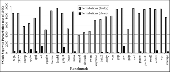
FIGURE 7.10 Perturbation in program segments. “Perturbations (clean)” are natural perturbations in a program. “Perturbations (faulty)” are induced perturbations. Reprinted with permission from Racunas et al. [16]. Copyright © 2007 IEEE.
As may be obvious by now, fault screeners are often incapable of distinguishing between natural and induced perturbations. Consequently, the use of such screeners most likely will require an accompanying recovery mechanism to avoid crashing a program in the presence of natural perturbations. Fault screeners are also incapable of catching faults that do not cause program perturbations, unless the fault coincides with an unrelated natural perturbation.
Research in Fault Screeners
Wang and Patel [22] and Racunas et al. [16] have studied several fault screeners and have shown that their screening accuracy may vary between 30% and 75%, as shown in Figure 7.11. Different fault screeners use different history and microarchitecture state to screen faults. For example, the ext-history screener tracks the history of past values seen by a static instruction, the dyn-range tracks the dynamic range of values seen by a static instruction, invar tries to identify bits that are invariant and seen by a static instruction, tlb screens faults based on tlb misses, and bloom uses a bloom filter [5] to screen for errors.

FIGURE 7.11 Accuracy of the fault screeners. Reprinted with permission from Racunas et al. [16]. db_avg is the average of database benchmarks SQL and TPCC. int_avg is the average of SPEC integer benchmarks shown to the right of db_avg. Copyright © 2007 IEEE.
Much research remains in the design and use of fault screeners to make them practical and useful in commodity microprocessors. Wang and Patel [22] studied other screeners, such as cache misses. However, screener design needs refinement and will remain an area of active research. The use of such screeners also needs further investigation. Wang and Patel [22] describe a design called RESTORE, which recovers a processor pipeline from an earlier checkpoint once it screens an error. Racunas et al. [16] propose recovering the pipeline state by flushing the pipeline and restarting it on screening an error.
Also, researchers are yet to evaluate the SER reduction from fault screening. Prior investigation has only evaluated the accuracy of fault screeners using fault injection into committed instruction state. This needs to be translated into an SER for bits in a chip. The difficulty is that the ACE analysis described in Chapter 3 cannot be used directly to evaluate the SER from fault screeners. This is because ACE analysis tries to abstract the SER from a single fault free execution. In contrast, fault screeners are only activated in the presence of a faulty symptom. Hence, without fault injection, it may be difficult to model the SER of a chip using a fault screener.
7.5 Backward Error Recovery with Fault Detection before Memory Commit
This section discusses design trade-offs for backward error recovery schemes that allow a processor to commit values to its architectural registers, but not to memory, prior to the fault detection point. In the schemes described in the last section in which the register commit was after the fault check, a processor could flush speculative pipeline state and restart execution from the existing architectural register file. In contrast, any backward error recovery scheme that allows values to be committed to the register file must provide a mechanism to roll back the register state.
The constraint of fault detection after the register commit point may often be imposed by the constraints of a specific design or implementation. For example, if the processor pipeline makes it difficult to add an extra pipe stage before the write-back stage where register values are committed, then the designer may be forced to do the fault detection after the register commit.
Once a fault is detected in such a backward error recovery scheme, a processor or a computing system needs a checkpoint to roll back the register state to. The method of generating this checkpoint can have a significant impact on how the system performs. There are typically two ways of generating such a checkpoint: incremental and periodic. In the incremental checkpointing, a system keeps a log of new values as and when they are generated. When these new values are committed to the register file, they are not checked for faults. However, they are checked for faults before they are committed to the log. On detecting a fault, this log is traversed in reverse order to regenerate the state of the system at the point where the fault was detected. In such a case, overhead to create the checkpoint is minimal, but the time to recover depends on how fast the error log can be traversed. This section describes a backward error recovery scheme that uses a history buffer as the log for incremental checkpointing.
In the periodic checkpointing, the processor periodically takes a snapshot of its state, which in this case is the processor register state. Before committing its state to a checkpoint, the processor or the system will typically ensure that the snapshot is fault free. Then, on detecting a fault, the processor reverts to the previous checkpoint and restarts execution. Periodically checkpointing the processor state reduces the need to do fault detection on every instruction execution (to guarantee that the checkpoint is fault free). However, it creates two new challenges. First, a large amount of state may need to be copied to create the checkpoint. Second, a large amount of state may be necessary to be compared to ensure that the newly created checkpoint is fault free. This section describes a scheme called fingerprinting that reduces the amount of state necessary to be compared to ensure a fault free checkpoint.
Because neither system—incremental nor periodic checkpointing—described in this section commits memory or I/O values outside the sphere of recovery, the output and input commit problems are solved relatively easily. No store or I/O operation is allowed until the corresponding operation is certified fault free, which solves the output commit problem. This also makes it easier to solve the input commit problem. Because stores are not committed till they pass their fault detection point and loads are idempotent, these systems can allow loads to be reissued by the processor after they roll back and recover from a previous checkpoint. Any uncached load must, however, be delayed until the load address is certified fault free.
Although incremental checkpointing and periodic checkpointing are discussed in the context of backward error recovery before memory commit, these techniques can also be extended to backward error recovery schemes that allow memory or I/O to commit before doing the fault check. Neither of these techniques, to the best of my knowledge, has been implemented in any commercial system.
7.5.1 Incremental Checkpointing Using a History Buffer
The key requirement to move the fault detection point of an instruction beyond its register commit point is to preserve the checkpointed state corresponding to an instruction. In SRTR, the processor frees up this state as soon as an instruction retires. Instead, an instruction could be retired, but its state must be preserved until the instruction passes its fault detection point. This state can be preserved via the use of a history buffer [12]. Smith and Pleszkun [18] first proposed a history buffer to support precise interrupts, but this section shows how it can be used for backward error recovery as well.
Structure of the History Buffer
The history buffer consists of a table with a number of entries. Each entry contains information pertinent to a retired instruction, such as the instruction pointer, the old destination register value, and the physical register to which the destination architecture register was mapped. The instruction pointer can be either the program counter or an implementation-dependent instruction number. The old destination value records the value of the register before this instruction rewrote it with its destination register value. Finally, the register mapping is also needed to identify the physical register that was updated. The number of entries in the history buffer is dependent on the implementation and must be chosen carefully to avoid stalls in the pipeline. The history buffer mechanism can work with many fault detection mechanisms, such as Lockstepping and SRT, which detect faults after register values have been committed.
Adding Entries to the History Buffer
When an instruction retires, but before it writes its destination register to the register file, an entry is created in the history buffer, and the entry’s contents are updated with the instruction pointer, old register value, and register map. Reading the old register value may require an additional read port in the register file. An additional read port may increase the size of the register file and/or increase its access time. Nevertheless, there are known techniques to avoid this performance loss (e.g., by replicating the register file). In effect, by updating the history buffer when an instruction retires, an incremental checkpoint of the processor state is created.
Freeing up Entries in the History Buffer
When a retired instruction passes its fault detection point, the corresponding entry in the history buffer is freed up. This is because the checkpoint corresponding to an instruction that has been certified to be fault free is no longer needed.
Recovery Using the History Buffer
If the fault detection mechanism detects a fault in a retired instruction, then the recovery mechanism kicks in. The following are the steps involved in recovering a processor that uses SRT as its fault detection mechanism:
![]() For both redundant threads, flush all speculative instructions that have not retired.
For both redundant threads, flush all speculative instructions that have not retired.
![]() For the trailing thread, flush its architectural state, including the architectural register file.
For the trailing thread, flush its architectural state, including the architectural register file.
![]() Reconstruct the correct state of the architectural register file of the leading thread using the existing contents of the register file and the history buffer. The architectural register file contains values up to the last retired instruction, which can be older than the instruction experiencing the fault. Hence, the values have to be rolled back to the state prior to the instruction with the fault. This can be accomplished by finding the oldest update to that register from the history buffer. This procedure is repeated for every register value that exists in the history buffer.
Reconstruct the correct state of the architectural register file of the leading thread using the existing contents of the register file and the history buffer. The architectural register file contains values up to the last retired instruction, which can be older than the instruction experiencing the fault. Hence, the values have to be rolled back to the state prior to the instruction with the fault. This can be accomplished by finding the oldest update to that register from the history buffer. This procedure is repeated for every register value that exists in the history buffer.
![]() Then the history buffer is flushed.
Then the history buffer is flushed.
![]() The contents of the leading thread’s register file are loaded into the trailing thread’s register file.
The contents of the leading thread’s register file are loaded into the trailing thread’s register file.
![]() Both threads are restarted from the instruction that experienced the fault.
Both threads are restarted from the instruction that experienced the fault.
7.5.2 Periodic Checkpointing with Fingerprinting
Unlike incremental checkpointing that incrementally builds a checkpoint, periodic checkpointing takes a snapshot of the processor state periodically. Although this reduces the necessity to do a fault detection on every instruction to ensure a fault free checkpoint, it does require copying a large amount of state to create the checkpoint and to ensure that the checkpoint is fault free.
Smolens et al. [19] introduced the concept of fingerprinting to reduce the amount of state that may be necessary to be compared for fault detection prior to checkpoint creation. In some ways, fingerprinting is a data compression mechanism. As and when each value is generated, it merges the generated value into a global running value or the fingerprint. Then, instead of comparing each and every value, the fingerprint can be compared prior to generating a checkpoint to ensure that the checkpoint is fault free.
Fingerprinting may be appropriate for a system that uses Lockstepping or RMT as its fault detection mechanism and where the communication bandwidth between the redundant cores, threads, or nodes is severely constrained. For example, if there are two processor chips or sockets forming the redundant pair, then the bandwidth between the chips may be limited. Copying state to create a checkpoint within a processor chip, however, may not incur a significant performance penalty since the communication for this copy operation may be limited to within a processor chip. But the state comparison requires off-chip communication, and off-chip bandwidth is often severely limited. Fingerprinting can help reduce the performance degradation from comparing large amounts of off-chip state. The rest of this subsection discusses fingerprinting and how it can help reduce the bandwidth requirements in the context of chip-external detection.
Fingerprint Mechanism
A fingerprint provides a concise view of the past and present program states. It contains a summary of the outputs of any new register values created by each executing instruction, the new memory values (for stores), and the effective addresses (for both loads and stores). By capturing all updates to architectural state, a fingerprint can ensure that it can help create a fault free checkpoint. It should be noted that this implementation of fingerprinting allows not only register values to be committed to the register file but also memory values to be committed to the processor caches. Nevertheless, the caches are not allowed to write back their modified data to main memory till the fault check has been done.
For fault detection with RMT processors, the fingerprint implementation must monitor only committed register values. However, for fault detection with Lockstepped processors, the fingerprint implementation can monitor both speculative and committed updates to the physical register file since both Lockstepped processors are cycle synchronized.
To create the fingerprint, Smolens et al. [19] propose hashing the generated values into a cyclic code. There are two key requirements for the code. First, the code must have a low probability of undetected faults. Second, the code should be small for both easy computation and low bandwidth comparison. For a p-bit CRC code, the probability of an undetected error is at most 2−p. Smolens et al. [19] used a 16-bit (p = 16) CRC code for their evaluation. A 16-bit CRC code has a 0.000015 probability that an error will go undetected. The reader is referred to Cyclic Redundancy Check, p. 178, Chapter 5, for a discussion on CRC codes.
Evaluation Methodology
To evaluate chip-external fault detection using fingerprinting for full-state comparison, Smolens et al. [19] simulated the execution of all 26 SPEC CPU 2000 benchmarks using SimpleScalar sim-cache [6] and two commercial workloads—TPC-C and SPECWeb—using Virtutech Simics. The simulated processor executed one IPC at a clock frequency of 1 GHz. The only microarchitecture parameter relevant to this evaluation was the level 2 (L2) cache configuration. The simulated processor has an inclusive 1-megabyte four-way set-associative cache with 64-byte lines.
The benchmarks used for evaluation can be classified into three categories: SPEC integer, SPEC floating point, and commercial workloads. Using the prescribed procedure from SimPoint [14], the authors simulated up to eight predetermined 100 million instruction regions from each SPEC benchmark’s complete execution trace. Using Simics, the authors ran two commercial workloads on Solaris 8: a TPC-C-like online transaction processing (OLTP) workload with IBM DB2 and a SPECWeb. The 100-client OLTP workload consisted of a 40-warehouse database striped across five raw disks and one dedicated log disk. The SPECWeb workload serviced 100 connections with Apache 2.0. The authors warmed both commercial workloads until the CPU utilization reached 100% and the transaction rate reached steady state. Once warmed, the commercial workloads executed for 500 million instructions.
Bandwidth Required for Full-State Comparison Using Lockstepped Processors
Smolens et al. [19] evaluated fault detection mechanisms based on their state-comparison bandwidth demand between mirrored processors. The bandwidth required for off-chip comparison is calculated as the sum of the address and databus traffic from off-chip memory requests. The average chip-external bandwidths generated by the three simulated application classes—SPEC CPU 2000 integer (SPEC CINT), SPEC CPU 2000 floating-point (SPEC CFP), and commercial—were
Whether Lockstepped or RMT systems can handle these full-state comparison bandwidths will depend on the exact system configuration.
Full-state comparison without fingerprinting uses the entire register file contents and all cache lines modified since the last checkpoint. The number of updated cache lines, however, grows slowly as the checkpoint interval is increased because of spatial locality. Assuming that the full-state comparison bandwidth amortizes over the entire checkpoint interval, the required bandwidth decreases as the checkpoint interval increases. In Figure 7.12, the average bandwidth requirement decreases sharply as the checkpoint interval increases. However, for the range of intervals compatible with I/O interarrival times of commercial workloads (hundred to thousands of instructions), the required bandwidth remains above several hundred megabytes per second.

FIGURE 7.12 Required bandwidth for full-state comparison (without fingerprinting) as a function of the checkpoint interval. Reprinted with permission from Smolens et al. [19]. Copyright © 2004 IEEE.
Fingerprinting provides a compressed view of the architectural state changes and significantly reduces this bandwidth pressure. Instead of comparing every instruction result, fingerprinting compares only two bytes per checkpoint interval. The bandwidth overhead for fingerprint comparison is thus orders of magnitude less than full-state comparison. Assuming a 1000-instruction checkpoint interval on a 1000-MIPS processor, fingerprinting consumes just 2 megabytes per second.
7.6 Backward Error Recovery with Fault Detection before I/O Commit
Until now this chapter discussed backward error recovery mechanisms that either do not commit any values outside the processor pipeline or commits values only to the architectural register files and processor caches. This subsection discusses backward recovery techniques that allow processor pipelines to commit values to main memory. By letting values to be committed to main memory, a system typically decreases the frequency, and the necessary bandwidth needed, with which the fault detection mechanism must be invoked. However, because the total amount of state held by main memory is several orders of magnitude greater than that of a processor register file, one needs recovery techniques that are different from those that rely on fault detection before memory commit.
This subsection discusses three such techniques. None of these has been implemented in a commercial system. The first is a log-based recovery mechanism. Specifically, an implementation that relies on an SRT processor’s LVQ mechanism to recover from errors is discussed. This implementation will commit newly generated memory values to main memory. On detecting a fault, it will roll back to a previous checkpoint maintained by the processor. Then it replays the execution from the checkpoint using load values already recorded in the LVQ but without committing memory values regenerated by stores. This implementation protects against faults within the processor pipeline as covered by the sphere of replication.
Two other techniques that are discussed are ReVive [15] and SafetyNet [20], which can recover from errors not only in the processor but also in the system itself, such as ones in the coherence protocol. Both these techniques generate and maintain system-wide checkpoints. On detecting a fault, both systems roll back to a previous checkpoint and restart execution. These techniques may provide more complete system-wide fault coverage than error coding techniques, such as ECC, since they can recover from errors in logic blocks, such as coherence controllers.
Generating system-wide checkpoints, however, can be tricky. If a processor or a node generates its own checkpoint independent of other processors or nodes, then it may lead to the “checkpoint inconsistency” problem. Given a fault, the system has to roll back the system—include all processor or nodes–to a consistent global state. A set of uncoordinated checkpoints may not provide a single consistent global state. For example, in Figure 7.13, node 0 sends a request for ownership for a memory block. Node 1 sends a transfer of ownership response back to node 0. At this point, both nodes 0 and node 1 take their local checkpoints. Then, node 0 receives the transfer of ownership response. The two local checkpoints shown in the figure are, however, inconsistent and cannot portray a single consistent global state. This is because node 1 thinks node 0 is the owner of the block, and node 0 thinks node 1 is the owner. Hence, checkpoint generation must be coordinated to generate a single global consistent state.

FIGURE 7.13 Demonstration of how local uncoordinated checkpoint can lead to inconsistent global state.
ReVive generates a single consistent global state by stopping all processing nodes and coordinating the generation of their individual checkpoints. In contrast, SafetyNet generates local checkpoints within a node but has enough intelligence built into the system to roll back to the appropriate local checkpoints that together make up a single global state.
The three systems solve the output and input commit problems slightly differently. For LVQ-based recovery, memory is outside the sphere of recovery. It only allows fault free stores to propagate to memory. However, because it allows multiple stores to commit to main memory since it created the checkpoint, it must record and replay all load values issued so far to ensure that on reexecution all the stores already committed are seen again. In contrast, for ReVive and SafetyNet memory is inside the sphere of recovery but I/O is not. They solve the output commit problem by not allowing I/O operations to commit until they can take a checkpoint. They solve the input commit problem by recording all external events, such as I/O interrupts, and by replaying them during reexecution after a rollback and recovery.
7.6.1 LVQ-Based Recovery in an SRT Processor
Log-based recovery is a well-established technique in the fault-tolerant systems area [7]. The concept applies to any system that is piecewise deterministic, i.e., in which execution consists of deterministic intervals separated by nondeterministic events (Figure 7.14). In this context, an event is considered nondeterministic if its execution is not determined entirely by the state inside the system. The state of a piecewise deterministic system at any point can be recreated, given an initial condition and a complete description of all nondeterministic events up to the desired point.

In the context of a processor’s transparent hardware recovery, the initial condition is the checkpointed architectural state, which includes any architecturally visible state, such as the architectural register file. The nondeterministic events are the following:
![]() Load values, since memory contents may be modified external to the sphere of replication by other processors or I/O devices
Load values, since memory contents may be modified external to the sphere of replication by other processors or I/O devices
![]() Timing-dependent operations, such as ones that read on-chip cycle counters.
Timing-dependent operations, such as ones that read on-chip cycle counters.
Interestingly, these events are identical to those required to maintain determinism between the leading and trailing threads in an SRT processor. As long as execution is deterministic, one can rely on both threads to follow the same execution path. Thus, it is exactly these same nondeterministic events that must be captured to keep the two threads consistent. This is the key insight behind log-based recovery in an SRT processor [17].
A designer may want to keep the checkpoint and the log fault free at creation and protected against transient faults (e.g., by ECC) to increase the fault coverage. After the completion and fault free validation of a checkpoint, both the previous checkpoint and all log entries prior to the new checkpoint can be discarded. The minimum checkpoint frequency is determined by the maximum available log storage and the maximum tolerable recovery latency.
The rest of this subsection describes the relationship between fault detection, checkpointing, and logging in SRT; how it can handle faults during regular execution (i.e., nonrecovery mode), during checkpoint creation, and in recovery mode; and how it can log load values and asynchronous interrupts.
Fault Detection, Checkpointing, and Logging
As discussed earlier (RMT within a Single-Processor Core, p. 227, Chapter 6), an SRT processor’s performance advantage over Lockstepping comes from doing the fault detection in the larger SRT-Memory sphere. Nevertheless, when checkpoints are created, it may also be necessary to check them for faults. That is, all new register values from the two redundant threads must be compared for mismatch. In the absence of a mismatch, they can be sent to the ECC-protected checkpoint storage. Because the checkpoint includes the state of the architectural register file, fault detection during checkpoint creation is similar to the checking required for the smaller SRT-Register’s sphere used in SRTR. However, the logging mechanism may avoid the performance problems suffered by SRTR due to limited slack. The log of external events, such as loads and asynchronous interrupts, ensures that the internal state of the machine at the point of a detected fault can be reproduced starting from the last checkpoint. This capability decouples the fault detection in SRT-Memory (used to verify data sent out externally) from the fault detection in SRT-Register (used to validate checkpoints).
This decoupling has two effects. First, checkpoint validation is not in the critical path of the program execution and thus can be done at leisure and in the background. Second, the log-based method does not have to create checkpoints corresponding to every output point. Rather, checkpoints can be created at any desired frequency. As discussed above, decreases in checkpoint frequency come at the cost of increased log storage and increased recovery latency.
Handling Faults in Nonrecovery Mode
In such a design, during normal execution (i.e., in a nonrecovery mode), an output mismatch for data exiting the SRT-Memory sphere (e.g., in a store address or in a value) indicates the presence of a fault. Then, both the leading- and the trailing-thread contexts are flushed because one cannot tell the thread that contains the fault. Both thread contexts are reloaded from the latest complete checkpoint. Then execution is resumed in recovery mode in which both the threads are driven by the saved event log.
This recovery mode is indistinguishable from the normal operation for the trailing thread but is distinct for the leading thread. Thus, for example, leading thread loads will be satisfied from the log rather than from the data cache, as in a normal operation. These recovery operations continue until all outputs generated since the checkpoint have been regenerated. This point is detected by maintaining a counter that tracks the number of outputs generated since the previous checkpoint, decrementing this counter for each regenerated output and exiting recovery mode when the counter reaches zero. The regenerated outputs, such as stores, are discarded because they have already been exposed outside the SRT-Memory.
Handling Faults during Checkpoint Creation
Checkpoint creation may occur either continuously in the background or at periodic intervals. Register values from both threads are compared for mismatch. In the absence of any mismatch, the outputs are committed to the external checkpoint storage. However, on a mismatch, both threads are flushed and restored to the previous complete checkpoint. Then the same procedure is followed as outlined earlier. It should be noted that external checkpoint storage must be capable of storing a full valid checkpoint until a subsequent checkpoint can be fully validated, potentially requiring twice the capacity of the architectural register file.
Handling Faults during Recovery Mode
Faults could occur during the recovery procedure itself. To detect these faults, one can run both the leading and trailing threads and compare both threads’ outputs that leave the SRT-Memory sphere. A detected fault during recovery mode could imply the presence of a permanent fault, when one could flag this to the OS to let it decide future action. Alternatively, if system designers believe that transient faults could be likely in such a situation, then they could simply restart both the redundant threads from the last checkpoint and run them off the saved event log.
Logging Loads Using the LVQ
As discussed earlier, the log required for recovery is a simple extension of the input replication mechanism already needed by an SRT processor to provide fault detection. Hence, one can leverage the input replication mechanisms, which recreate nondeterministic events from the leading thread in the trailing thread, to handle these same events for recovery. RMT replicates load values from the leading to the trailing thread using an LVQ. The LVQ is a queue of load values as seen by the leading thread. Loads from the trailing thread obtain their values from the LVQ instead of the data cache.
Extending the LVQ for recovery consists of maintaining LVQ entries after the trailing thread has consumed them until a checkpoint is completed. If checkpoints are frequent, entries may be kept in the same physical LVQ structure used for input replication. Otherwise, a larger log may be required, when LVQ entries may be copied from the primary LVQ to a separate recovery-only LVQ structure. Because the performance of recovery may not be critical, the recovery LVQ may be larger, slower, and farther from the core than the replication LVQ. Even if a single physical structure is used, it is useful to logically distinguish replication LVQ entries (which have not been consumed by the trailing thread) from recovery LVQ entries (which have been consumed by the trailing thread but are not yet incorporated in the latest checkpoint).
Logging Asynchronous Interrupts
Asynchronous interrupts are replicated in an SRT processor by logging the point in the dynamic instruction stream at which the interrupt is taken in the leading thread and by generating the interrupt at the same point in the trailing thread, or by forcing the thread copies to synchronize to the same execution point and delivering the interrupt simultaneously. In the former scenario, asynchronous interrupts could be logged and replayed in the same manner as loads. The mechanism for generating interrupts from the log can leverage the logic used to generate interrupts in the trailing thread in a normal operation. In the latter scenario, interrupts are not stored and transferred between threads, so there is no mechanism to leverage. In this case, a more direct approach would be to force a check point after the threads synchronize, eliminating the need to log interrupt events. Other nondeterministic events should be addressed on a case-by-case basis, though this framework of leveraging the replication mechanism for logging (or forcing checkpoints) should apply in general.
7.6.2 ReVive: Backward Error Recovery Using Global Checkpoints
ReVive is a backward error recovery technique targeted for cache-coherent shared-memory multiprocessors [15]. Such a shared-memory multiprocessor is composed of multiple nodes. Each node consists of a processor, caches, and its local main memory. The caches are kept coherent using a cache coherence protocol. Unlike the LVQ-based recovery in SRT, ReVive maintains system-wide global checkpoints that can help the system recover from errors in either the memory system or the coherence protocol logic.
ReVive has three basic components: distributed parity to detect faults in memory, an undo log that tracks the first writes to memory locations after a consistent checkpoint is established, and a method to create a globally consistent checkpoint. In the LVQ-based recovery just described, the SRT processor periodically copies its architectural state to a separate checkpoint memory. This maybe feasible since the architectural state is typically small, consisting of architectural registers and processor state. Then it logs nondeterministic events and input load values to replay them later during recovery.
In contrast, ReVive uses the entire memory itself as its checkpoint since copying it may be infeasible. First, ReVive ensures that the entire memory across the system is in a consistent state. This may require flushing the processor caches, so that individual processors do not have a more recent up-to-date copy of modified blocks. ReVive’s log keeps track of the first memory write to any memory location since the consistent global state was created. On detecting a fault, ReVive uses the combination of the current memory state and the undo log to roll back the entire memory state of the system to a globally consistent state.
Distributed Parity
ReVive implements distributed parity to both detect faults and recover from errors in its distributed memory, which serves both as the main memory and as a part of the checkpoint. The scheme is similar to what is used in RAID (Redundant Array of Inexpensive Disks) systems. As Figure 7.15 shows, in ReVive, memory is organized as parity groups, where a memory block in one node contains the parity bits corresponding to the data bits for the other nodes. Thus, a parity bit P in the memory block holding parity can be computed as P = A XOR B XOR C, where A, B, and C are the corresponding data bits in each of the other memories.

FIGURE 7.15 Parity groups in ReVive’s distributed memory protected with parity. Shaded boxes represent parity bits, whereas boxes not shaded represent data bits. Each bit in the shaded parity box is an XOR of the corresponding data bits in the same parity group.
When a memory write occurs in a specific memory block, the corresponding controller sends the XOR of the original parity bits and the newly created parity bits for the memory block that was just written to the memory that holds its parity bits. Assume the new parity bit is C′. Then the controller holding C sends an update U = C XOR C′ to the controller with the parity bit. The reader can easily verify that the controller with the parity bits can compute the new parity bit simply as P′ = P XOR U. Using this distributed parity scheme, ReVive can completely recover from single-bit transient faults in its memory system and from the complete loss of a node’s entire memory.
Logging Writes
ReVive must keep track of the first write to any memory block since the last checkpoint was created. When it detects a write, it copies the old value into a log and writes the new value to memory. Then, on detecting a fault, it can simply use the log to reset the values of all blocks to recreate the checkpoint and restart execution.
Typically, cache-coherent, shared-memory multiprocessors implement a single-writer invalidation protocol, which allows multiple readable copies of a memory block, but only one node can write the block at any time. To write a block, a node must have the only copy of the block and must be its exclusive owner. Before a block transitions from readable to exclusive, the corresponding node must request an exclusive write access to this block. This makes it easy for a memory controller to detect a node’s intention to write a memory block. At that point, the memory controller can save the old value of the memory block in the log.
To only log the first write to block after a checkpoint, ReVive augments its blocks with an additional bit—called the log bit–beyond what may be needed by the coherence protocol. The log bit tracks first writes to a block after a checkpoint. If the log bit is set, then ReVive will not copy the block’s old value to the log when a write request comes. The log bits are reset when a checkpoint is created.
Global Checkpoint Creation
To create the global checkpoint, ReVive follows a simple two-phase protocol. First, all processors and nodes synchronize and flush all their caches to write all modified data back to memory. Then the processors synchronize again to ensure that all processors have completed writing all their data back to memory. All the log bits are also cleared at this time. The checkpoint is now established, and all processors can resume execution. Because an error may occur during the creation of a checkpoint, ReVive does not discard the old log till all processors complete the two-phase protocol.
7.6.3 SafetyNet: Backward Error Recovery Using Local Checkpoints
Like ReVive, SafetyNet is a backward error recovery scheme targeted to recover from errors in a cache-coherent, shared-memory multiprocessor [20]. SafetyNet’s logging scheme is similar to ReVive’s. Unlike ReVive, however, SafetyNet generates local checkpoints in a way that allows it to create a globally consistent state, if a roll-back is necessary. In the background, SafetyNet coordinates different local checkpoints to ensure that there always exists a globally consistent checkpointed state that the entire system can roll back to. Once it establishes such a recovery point, it frees up any prior local checkpoints. Because SafetyNet takes local checkpoints, it can create checkpoints much faster than ReVive. The SafetyNet scheme is, however, more complex to implement than ReVive.
Creating Consistent Checkpoints
In SafetyNet, all nodes periodically take local checkpoints at a globally synchronous logical time. The local checkpoint is a combination of the processor’s architectural state and a log of first memory writes since the last checkpoint was initiated. To ensure that the local checkpoints reflect a consistent system state, SafetyNet exploits the key insight that, in retrospect, a coherence transaction appears logically atomic once the entire coherence transaction has completed. A transaction’s point of atomicity can be established when the previous owner of the requested block processes the request. For example, in Figure 7.16, the point of atomicity could be T1. Node 0 sends a request to the previous owner (Node 1). Node 1 establishes the point of atomicity at T1 and forwards its last checkpoint number (checkpoint #2) to Node 0 as its checkpoint number for the point of atomicity. Node 0, the requestor, does not learn the location of the atomicity point until it receives the response that completes the transaction. To ensure that the system never recovers to the “middle” of a transaction, the requestor does not advance the recovery point until all its outstanding transactions complete successfully. After completion, the transaction appears atomic.

FIGURE 7.16 Example of checkpoint coordination in SafetyNet. Reprinted with permission from Sorin et al. [20]. Copyright © 2002 IEEE.
Advancing the Global Recovery Point
At any point of time, SafetyNet maintains a combination of local checkpoints that constitute a consistent global state, which is referred to as the global recovery point. As each node creates local checkpoints, one must advance the global recovery point, so that each node can free up the storage for its prior local checkpoints. Further, any I/O operation can be performed only after a global recovery point is established.
For a checkpoint interval to be fault free, no fault detector in the system should signal an error and every transfer of ownership in that interval must complete successfully. This ensures that the data were transferred fault free to the requestor. Once every component has independently declared that it has received fault free data in response to all its requests in the interval before the checkpoint, the global recovery point can be advanced. At this point, all transactions prior to this checkpoint have had their points of atomicity determined. Then the state for the prior recovery point can be deallocated lazily. One can establish this global recovery point in the background to avoid slowing down the main computation.
The latency to establish the global recovery point depends on the fault detection latency. Some faults that manifest themselves as corrupted messages can be caught immediately through CRC codes, which are often used to protect network messages. Other faults, such as dropped messages, may have to rely on timeout latency that can be many traversals of the interconnect.
7.7 Backward Error Recovery with Fault Detection after I/O Commit
Including I/O devices in the sphere of recovery is a difficult problem and is hard to tackle in hardware. This is because I/O operations can have side effects, which may be hard to control and recover from. For example, an uncached store to an I/O device may trigger the device to send an incorrect message to a terminal, which cannot be recovered from. It is often difficult for a computing system to recover from such an operation.
There are, however, scenarios in which an application can recover even after it commits to an I/O device. For example, databases routinely maintain recovery logs that can be used to recover from incorrect disk operation. These recovery operations are, however, often handled on a per-application basis and in software. Nakamo et al. [13] discuss how disk operations can be rolled back since disk reads are idempotent.
Networking stacks, such as TCP/IP, are allowed to send duplicate messages into the network. This is because if the sender does not receive an acknowledgement, it can send a duplicate copy of the message to the receiver. The same mechanism can be used to send a duplicate message after any operation has been rolled back. Chapter 8 discusses such software-controlled backward error recovery techniques.
7.8 Summary
Fault detection mechanisms either remove any SDC from a system or convert them to DUE. Error recovery mechanisms can reduce or eliminate both the SDC and DUE rates of a system. Broadly, error recovery mechanisms can be classified into forward and backward error recovery mechanisms.
In a forward error recovery, a system can continue executing from its current state after a fault is detected. The forward error recovery schemes usually maintain a redundant, up-to-date error-free state from which the system can continue execution. In contrast, a backward error recovery scheme usually rolls back to a previous error-free state of a system. Such states are referred to as checkpoints and can be generated incrementally or periodically by a system.
There are four options for implementing forward error recovery in hardware: fail-over systems, DMR, TMR, and pair-and-spare. Each of these systems has incrementally smaller downtime compared with the previous one. Fail-over systems typically consist of a mirrored pair of computing slices denoted as the primary and secondary. When the primary slice detects a fault, the secondary slice takes over execution with some state correction (e.g., restarting the failed process).
A DMR system detects faults by comparing outputs from two redundant slices of execution. Further, if an internal error checker, such as a parity checker, fires within one of the slices, then the output comparator can precisely determine the slice that is in error. Then, by copying the correct state from the fault free slice to the faulty slice, the DMR system can recover from the error.
A TMR system extends the concept of DMR by running three redundant slices of execution. The output comparator votes on the output that is correct. If outputs from one of the redundant slices are faulty, then the TMR system freezes that slice but can continue execution in degraded DMR mode with the other two fault free slices. Eventually, the correct state must be copied from the fault free slices to the faulty slice to reintegrate the faulty slice into the TMR system.
Finally, pair-and-spare extends the TMR concept by running four redundant slices. The primary pair is the one that commits to system state. The secondary pair keeps its state up-to-date with the primary pair. When the primary pair detects a fault, it transfers execution to the secondary pair.
Unlike forward error recovery schemes, a backward error recovery scheme rolls back execution to a prior fault free state referred to as a checkpoint. What constitutes a checkpoint depends on the fault detection scheme. Four options are possible: fault detection before register commit, fault detection before memory commit, fault detection before I/O commit, and fault detection after I/O commit. Fault detection after I/O commit is typically achieved in software (not discussed in this chapter). If the fault is detected before registers are committed, then existing techniques that a processor uses to recover from a misspeculation, such as a branch misprediction, can be used to recover from a transient fault.
If the fault is detected after registers are committed, but before memory is committed, then the recovery scheme needs a mechanism to checkpoint the register state. This can be done incrementally through the use of a history buffer that logs all register updates. Alternatively, this can be done periodically by taking snapshots of the register state. Periodic checkpointing may require significant output comparison bandwidth to ensure that the checkpoint is fault free. This can be reduced through a state-compression technique known as fingerprinting.
If the fault is detected after memory is committed, then the system must support a mechanism to roll back memory state. Memory state is typically much larger than register state, so it may be difficult to take a checkpoint of memory state. Instead, systems typically maintain a log of memory values received from the system since the prior register checkpoint. During recovery, the system can then replay execution, starting at the register checkpoint and using the log of memory values as inputs to the execution stream. Distributed memory machines impose an additional problem in which checkpoints must be globally consistent across an entire system. This can be achieved by coordinating checkpoint generation across the individual nodes of a distributed system.
7.9 Historical Anecdote
One of Stratus Technologies’ customers had requested an automatic reboot capability in the event of a system hang. This is because the customer had many unattended sites that would benefit from such an automatic reboot. Stratus did implement such a facility through something called a dead man timer [10]. The computer automatically rebooted if the dead man timer was not periodically reset by the software running on it. Many of Stratus’ customers who were not aware of this dead man timer were not running the appropriate software to reset it. They experienced many mysterious crashes for months. Thus, a capability that Stratus implemented to recover a system from a system hang ended up crashing the system itself.
Stratus did not notice this problem due to a number of issues. The dead man timer was not well documented and was designed in a somewhat ad hoc fashion. It did not record a log and therefore operators had no way of telling if the dead man timer had reset the system. The signal to drive the timer was only 1 bit wide, nonredundant, and unchecked. Consequently, a 1-bit error in the transmission of the signal could also activate the timer mechanism. The timer design was not also subject to usual design reviews that engineering companies normally implement. Once Stratus was notified of the problem, its engineers fixed the problem in a week. Since then, Stratus has imposed strict review and controls to ensure that new features do not cause similar problems.
References
Ando H., Yoshida Y., Inoue A., Sugiyama I., Asakawa T., Morita K., Muta T., Motokurumada T., Okada S., Yamashita H., Satsukawa Y., Konmoto A., Yamashita R., Sugiyama H. A 1.3 GHz Fifth Generation SPARC Microprocessor. 2003 IEEE Solid State Circuits Conference (ISSCC). 2003:1896–1905.
Barlett J., Bartlett W., Carr R., Garcia D., Gray J., Horst R., Jardine R., Lenoski D., Mcguire D. Fault Tolerance in Tandem Computer Systems. In: Technical Report 90.5, Part Number 40666. Hewlett-Packard; May 1990.
Bartlett W., Spainhower L. Commercial Fault Tolerance: A Tale of Two Systems. IEEE Transactions on Dependable and Secure Computing. January–March 2004;Vol. 1(No. 1):87–96.
Bernick D., Bruckert B., Vigna P.D., Garcia D., Jardine R., Klecka J., Smullen J. NonStop® Advanced Architecture. Proceedings of the International Conference on Dependable Systems and Networks (DSN). 2005:12–21.
Bloom B. Space/Time Trade-offs in Hash Coding with Allowable Errors. Communications of the ACM. July 1970;Vol. 13(No. 7):422–426.
Burger D., Austin T.M. The Simplescalar Tool Set, Version 2.0. In: Technical Report 1342. Computer Sciences Department, University of Wisconsin-Madison; June 1997.
Elnozahy M., Alvisi L., Wang Y.-M., Johnson D.B. A Survey of Rollback-Recovery Protocols in Message-Passing Systems. In: Technical Report CMU-CS-99-148. School of Computer Science, Carnegie Mellon University; June 1999.
Gomaa M.A., Vijaykumar T.N. Opportunistic Fault Detection. 32nd Annual International Symposium on Computer Architecture. 2005:172–183.
Gomaa M.A., Scarbrough C., Vijaykumar T.N., Pomeranz I. Transient Fault-Recovery for Chip Multiprocessors. 30th Annual International Symposium on Computer Architecture. June 2003:96–109.
Green P.A., Jr. Observations From 16 Years at a Fault-Tolerant Computer Company. 15th Symposium on Reliable Distributed Systems. 1996:162–164.
Hangal S., Lam M. Tracking Down Software Bugs Using Automatic Anomaly Detection. International Conference on Software Engineering, ICSE′02. May 2002:291–301.
Mukherjee S.S., Reinhardt S.K., Emer J.S. Incremental Checkpointing in a Multi-Threaded Architecture, August 29, 2003. United States Patent Application, Filed
Nakamo J., Montesinos P., Gharachorloo K., Torrellas J. ReVive I/O: Efficient Handling of I/O in Highly-Available Rollback-Recovery Servers. 12th Annual International Symposium on High-Performance Computer Architecture (HPCA). 2006:200–211.
Perelman E., Hamerly G., Van Biesbrouck M., Sherwood T., Calder B. Using SimPoint for Accurate and Efficient Simulation. ACM SIGMETRICS, the International Conference on Measurement and Modeling of Computer Systems. June 2003:318–319.
Prvulovic M., Zhang Z., Torrellas J. ReVive: Cost-EffectiveArchitectural Support for Rollback RecoveryinShared-Memory Multiprocessors. 29th Annual International Symposiumon Computer Architecture (ISCA). 2002:111–122.
Racunas P., Constantinides K., Manne S., Mukherjee S.S. Perturbation-Based Fault Screening. 13th Annual International High-Performance Computer Architecture (HPCA). February 2007:169–180.
Reinhardt S.K., Mukherjee S.S., Emer J.S. Periodic Checkpointing in a Redundantly MultiThreaded Architecture, August 29, 2003. United States Patent Application, Filed
Smith J.E., Pleszkun A.R. Implementation of Precise Interrupts in Pipelined Processors. 12th International Symposium on Computer Architecture. 1985:291–299.
Smolens J.C., Gold B.T., Kim J., Falsafi B., Hoe J.C., Nowatzyk A.G. Fingerprinting: Bounding Soft-Error Detection Latency and Bandwidth. IEEE Micro. November 2004;Vol. 24(No. 6):22–29.
Sorin D.J., Martin M.M.K., Hill M.D., Wood D.A. SafetyNet: Improving the Availability of Shared Memory Multiprocessors with Global Checkpoint/Recovery. International Symposium on Computer Architecture (ISCA). May 2002:123–134.
Vijaykumar T.N., Pomeranz I., Cheng K. Transient Fault Recovery Using Simultaneous Multithreading. 29th Annual International Symposium on Computer Architecture. May 2002:87–98.
Wang N.J., Patel S.J. ReStore: Symptom-Based Soft Error Detection in Microprocessors. IEEE Transactions on Dependable and Secure Computing. July–September 2006;Vol. 3(No. 3):188–201.
Weaver C., Emer J., Mukherjee S.S., Reinhardt S.K. Techniques to Reduce the Soft Error Rate of a High-Performance Microprocessor. 31st Annual International Symposium on Computer Architecture (ISCA). 2004:264–275.