
Chapter 12. Applications of Discrete-Time Signals and Systems
Nullius in verba (Take nobody's word for it).
Motto of the Royal Society, Britain's 350-year-old science fraternity
12.1. Introduction
In this chapter we will present applications of the theory of discrete-time signals and systems to three important areas: digital signal processing, digital control, and digital communications. The material in this chapter is meant to be a more motivational than detailed presentation. We encourage our readers to look for the details in excellent textbooks in these three areas 54, 22 and 16.
Given the advances in digital technologies and computers, processing of signals is being done mostly digitally. Early results in sampling, analog-to-digital conversion, and the fast computation of the output of linear systems using the Fast Fourier Transform (FFT) made it possible for digital signal processing to become a technical area on its own. (The first books in this area 63 and 54 come from the mid-1970s.) Although the origins of the FFT have been traced back to the German mathematician Gauss in the early 1800s, the modern theory of the algorithm comes from the 1960s. It should be understood that the FFT is not yet another transform, but an efficient algorithm to compute the discrete Fourier transform (DFT), which we covered in Chapter 10.
Analog classic control systems can be implemented digitally using analog-to-digital and digital-to-analog converters and computers to implement the control laws. The theory of sampled data shows the connection between the Laplace and the Z-transform. The difficulty in the analysis of these systems is the mixing of continuous- and discrete-time signals.
Digital communication systems provide a more efficient way to communicate information than analog communication systems, but they are more demanding in terms of bandwidth. As indicated before, digital communications began with the introduction of pulse code modulation (PCM). Telephony and radio using baseband and band-pass signals have converged into wireless communications. Many of the principles of analog communications have remained, but its implementation has changed from analog to digital with slightly different objectives. Efficient use of the radio spectrum and efficient processing have become the objectives of modern wireless communication systems such as spread spectrum and orthogonal frequency-division multiplexing, which we introduce here.
12.2. Application to Digital Signal Processing
In many applications, such as speech processing or acoustics, one would like to digitally process analog signals. In practice, this is possible by converting the analog signals into binary signals using an analog-to-digital converter (ADC), and if the output is desired in analog form a digital-to-analog converter (DAC) is used to convert the binary signal into a continuous-time signal. Ideally, if no quantization is considered and if the discrete-time signal is converted into an analog signal by sinc interpolation the system can be visualized as in Figure 12.1.
 |
| Figure 12.1 |
Viewing the whole system as a black box with an analog signal x(t) as input, and giving as output also an analog signal y(t), the processing can be seen as a continuous-time system with a transfer function G(s). Under the assumption of no quantization, the discrete-time signal x[n] is obtained by sampling x(t) using a sampling period determined by the Nyquist sampling condition. Likewise, considering the transformation of a discrete-time (or sampled signal) y[n] into a continuous-time signal y(t) by means of the sinc interpolation, the ideal DAC is an analog low-pass filter that interpolates the discrete-timesamples to obtain an analog signal. Finally, the discrete-time signal x[n] is processed by a discrete-time system with transfer function H(z), which depends on the desired transfer function G(s).
Thus, one can process discrete- or continuous-time signals using discrete systems. A great deal of the computational cost of this processing is due to the convolution sum used to obtain the output of the discrete system. That is where the significance of the FFT algorithm lies. Although the DFT allows us to simplify the convolution to a multiplication, it is the FFT that as an algorithm provides a very efficient implementation of this process. In the next section, we will introduce you to the FFT and provide some of the basics of this algorithm for you to understand its efficiency.
12.2.1. Fast Fourier Transform
Comparing the equations for the DFT and the inverse DFT, or IDFT
(12.1)

(12.2)

Two issues used to assess the complexity of an algorithm are:
■ Total number of additions and multiplications: Typically, the complexity of a computational algorithm is assessed by determining the number of additions and multiplications it requires. The direct calculation of X[k] using Equation (12.1) for k = 0, …, N − 1 requires N × N complex multiplications, and N × (N − 1) complex additions. Computing the number of real multiplications and real divisions needed, it is found that the total number of these operations is of the order of N2.
■ Storage: Besides the number of computations, the required storage is an issue of interest.
Radix 2 FFT Algorithm
In the following, we consider the basic algorithm for the FFT. We assume that the FFT length is N = 2γ for an integer γ > 1. Excellent references on the DFT and the FFT are Briggs and Henson [10] and Brigham [11]
The FFT algorithm:
■ Uses the fundamental principle of “divide and conquer”: Dividing a problem into smaller problems with similar structure, the original problem can be successfully solved by solving each of the smaller problems.
■ Takes advantage of periodicity and symmetry properties of  :
:
(a) Periodicity: is periodic of period N with respect to n, and with respect to k—that is,

(b) Symmetry: The conjugate of  is such that
Decimation-in-Time Algorithm
Applying the divide-and-conquer principle, we express X[k] as

From the definition of  we have that

(12.3)
Although it is clear how to compute the values of X[k] for k = 0, …, (N/2) − 1 as
(12.4)
(12.5)
(12.6)

Repeating the above computation for Y[k] and Z[k] we can express it in a similar matrix form until we reduce the process to 2 × 2 matrices. While performing these computations, the ordering of x[n] is changed. This scrambling of x[n] is obtained by a permutation matrix PN (with 1 and 0 entries indicating the resulting ordering of the x[n] samples). If N = 2γ, the XN vector, containing the DFT terms X[k], is obtained as the product of γ matrices Ai and the permutation matrix. That is,
(12.7)

Consider the decimation-in-time FFT algorithm for N = 4. Give the equations to compute the four DFT values X[k], k = 0, …, 3 in matrix form.
Solution
If we compute the DFT of x[n] directly we have that


Separating the even- and the odd-numbered entries of x[n], we have


Now we have that


Reordering the x[n] entries we have


12.2.2. Computation of the Inverse DFT
The FFT algorithm can be used to compute the inverse DFT without any changes in the algorithm. Assuming the input x[n] is complex (x[n] being real is a special case), the complex conjugate of the inverse DFT equation, multiplied by N, is
(12.8)

Remark
In the FFT algorithm the 2N memory allocations for the complex input (one allocation for the real part and another for the imaginary part of the input) are the same ones used for the output. Each step usesthe same locations. Since X[k] is typically complex, to have identical allocation with the output, the input sequence x[n] is assumed to be complex. If x[n] is real, it is possible to transform it into a complex sequence and use properties of the DFT to obtain X[k].
12.2.3. General Approach of FFT Algorithms
Although there are many algorithmic approaches to the FFT, the initial idea was to represent the finite one-dimensional signal x[n] as a two-dimensional array. This can be done by representing the length N of x[n] as the product of smaller integers, provided N is not prime. If N is prime, the DFT computation is done with the conventional formula, as the FFT does not provide any simplification. However, in that case we could attach zeros to the signal (if the signal is not periodic) to increase its length to a nonprime number. This factorization approach has historic significance as it was the technique used by Cooley and Tukey, the authors of the FFT.
Suppose N can be factored as N = pq; then the frequency and time indices k and n in the direct DFT can be written as

(12.9)

The decimation-in-time FFT presented before may be viewed in this framework by letting q = 2 and p = N/2, where as before N = 2γ is even. We then have using  ,
,
(12.10)

Factoring N = 2 × N/2 corresponds to one step of the decimation-in-time method. If we factor N/2 as N/2 = (2)(N/4), we would obtain the second step in the decimation-in-time algorithm. If N = 2γ, this process is repeated γ times or until the length is 2.
Remark
A dual of the decimation-in-time FFT algorithm is the decimation-in-frequency method.
The Modern FFT
A paper by James Cooley, an IBM researcher, and Professor John Tukey from Princeton University [15] describing an algorithm for the machine calculation of complex Fourier series appeared in Mathematics of Computation in 1965. Cooley, a mathematician, and Tukey, a statistician, had in fact developed an efficient algorithm to compute the discrete Fourier transform (DFT), which will be called the FFT. Their result was a turning point in digital signal processing: The proposed algorithm was able to compute the DFT of a sequence of length N using N log N arithmetic operations, much smaller than the N2 operations that had blocked the practical use of the DFT. As Cooley indicated in his paper “How the FFT Gained Acceptance”[14], his interest in the problem came from a suggestion from Tukey on letting N be a composite number, which would allow a reduction in the number of operations of the DFT computation.
The FFT algorithm was a great achievement for which the authors received deserved recognition, but also benefited the new digital signal processing area, and motivated further research on the FFT. But as in many areas of research, Cooley and Tukey were not the only ones who had developed an algorithm of this class. Many other researchers before them had developed similar procedures. In particular, Danielson and Lanczos, in a paper published in the Journal of the Franklin Institute in 1942 [19], proposed an algorithm that came very close to Cooley and Tukey's results. Danielson and Lanczos showed that a DFT of length N could be represented as a sum of two N/2 DFTs proceeding recursively with the condition that N = 2γ. Interestingly, they mention that (remember this was in 1942!):
Adopting these improvements the approximation time for Fourier analysis are: 10 minutes for 8 coefficients, 25 minutes for 16 coefficients, 60 minutes for 32 coefficients, and 140 minutes for 64 coefficients.
Consider computing the FFT of a signal of length N = 23 = 8 using the decimation-in-time algorithm.
Solution
Letting N = qp = 2 × 4, we then have that


 |
| Figure 12.2 |
If we let y[n] = x[2n] and z[n] = x[2n + 1], n = 0, …, 3, we can then repeat the above procedure by factoring 4 = pq = 2 × 2 and expressing Y[k] and Z[k] as we did for X[k]. Thus, we have


In this example we wish to compare the efficiency of the FFT algorithm with that of our algorithm dft.m that computes the DFT using its definition. Consider the computation of the FFT and the DFT of a signal consisting of ones of increasing lengths N = 2r, r = 8, …, 11, or 256 to 2048.
Solution
To compare the algorithms we use the following script. The MATLAB function cputime measures the time it takes for each of the algorithms to compute the DFT of the sequence of ones.
%%%%%%%%%%%%%%
% example 12.3
% fft vs dft
%%%%%%%%%%%%%%
clf; clear all
time = zeros(1,4); time1 = time;
for r = 8:11,$$
N(r) = 2 ^ r;
i = r - 7;
t = cputime;
fft(ones(1,N(r)),N(r));
time(i) = cputime - t;
t = cputime;
dft(ones(N(r),1),N(r));
time1(i) = cputime - t;
end
%%%%%%%%%%%
% function dft
%%%%%%%%%%%
function X = dft(x,N)
n = 0:N - 1;
for k = 1:N - 1,
W = [W; exp(-j ∗ 2 ∗ pi ∗ n ∗ k/N)];
end
X = W ∗ x;
The results of the comparison are shown in Figure 12.3. Notice that to make the Computer Processing Unit (CPU) time for the FFT comparable with that of the dft algorithm, it is multiplied by 104, illustrating how much faster the FFT is compared to the computation of the DFT from its definition.

The convolution sum is computationally very expensive. Compare the CPU time used by the MATLAB function conv, which is used to compute the convolution sum in the time domain, with the CPU time used by an implementation of the convolution sum in frequency using the FFT. Recall that the frequency implementation requires computing the DFT of the signals being convolved, their multiplication, and finally the computation of the IDFT to the final convolution result.
Solution
To illustrate the efficiency in computation provided by the FFT in computing the convolution sum we compare the CPU times used by the conv function and the implementation of the convolution sum using the FFT. As indicated before, the convolution of two signals x[n], and y[n] of lengths N and M is obtained in the frequency domain by following these three steps:
■ Compute the DFTs X[k], Y[k] of x[n], and y[n] of length M + N − 1.
■ Multiply these complex DFTs to get X[k]Y[k] = U[k].
■ Compute the IDFT of U[k] corresponding to the convolution x[n] ∗ y[n].
Implementing the DFT and the IDFT with the FFT algorithm it can be shown that the computational complexity of the above three steps is much smaller than that of computing the convolution sum directly using the conv function.
To demonstrate the efficiency of the FFT implementation we consider the convolution of a signal, for increasing lengths, with itself. The signal is a sequence of ones of increasing length of 1000 to 10,000 samples. The CPU times used by the functions conv and the FFT three-step procedure are measured and compared for each of the lengths. The CPU time used by conv is divided by 10 to be able to plot it with the CPU of the FFT-based procedure shown in the following script. The results are shown in Figure 12.4.
 |
| Figure 12.4 |
%%%%%%%%%%%%%
% example 12.4
% conv vs fft
%%%%%%%%%%%%%
time1 = zeros(1,10);time2 = time1;
for i = 1:10,
NN = 1000 ∗ i;
x = ones(1,NN);
t0 = cputime;
y = conv(x,x); % convolution using conv
time1(i) = cputime-t0;
t1 = cputime;
X = fft(x,M); X = fft(x,M); Y = X. ∗ X; y1 = ifft(Y); % convolution using fft
time2(i) = cputime-t1
sum(y-y1) % check conv and fft results coincide
pause % check for small difference
end
Gauss and the FFT
Going back to the sources used by the FFT researchers it was discovered that many well-known mathematicians had developed similar algorithms for different values of N. But that an algorithm similar to the modern FFT had been developed and used by Carl Gauss, the German mathematician, probably in 1805, predating even Fourier's work on harmonic analysis in 1807, was an interesting discovery—although not surprising [31]. Gauss has been called the “prince of mathematicians” for his prodigious work in so many areas of mathematics, and for the dedication to his work. His motto was Pauca sed matura (few, but ripe); he would not disclose any of his work until he was very satisfied with it. Moreover, as it was customary in his time, his treatises were written in Latin using a difficult mathematical notation, which made his results not known or understood by modern researchers. Gauss's treatise describing the algorithm was not published in his lifetime, but appeared later in his collected works. He, however, deserves the paternity of the FFT algorithm.
The developments leading to the FFT, as indicated by Cooley [14], point out two important concepts in numerical analysis (the first of which applies to research in other areas): (1) the divide-and-conquer approach—that is, it pays to break a problem into smaller pieces of the same structure; and (2) the asymptotic behavior of the number of operations. Cooley's final recommendations in his paper are worth serious consideration by researchers in technical areas:
■ Prompt publication of significant achievements is essential.
■ Review of old literature can be rewarding.
■ Communication among mathematicians, numerical analysts, and workers in a wide range of applications can be fruitful.
■ Do not publish papers in neoclassic Latin.
12.3. Application to Sampled-Data and Digital Control Systems
Most control systems being used today use computers and ADCs and DACs. Control systems where continuous- and discrete-time signals appear are called sample-data systems. The analysis of these systems is more complicated than that of either continuous- or discrete-time systems, given the mixed signals in the system. In the following analysis we will ignore the effect of the quantizer and the coder, so that we are not considering digital control systems, but rather sampled-data or discrete control systems. Understanding the effects of sampling and the conversion of signals from continuous to discrete and back from discrete to continuous is very important in obtaining a discrete-time system from a sampled-data control system.
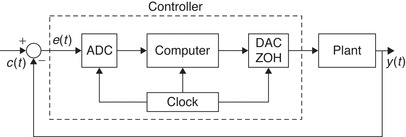
Consider the relation between a continuous control system and its implementation using a computer as shown in Figure 12.5. In the continuous-feedback system, the controller responds to an error signal e(t), which is the difference between a reference input signal c(t) and the system output y(t), attempting to change the dynamics of an analog plant. A digital realization of this continuous-feedback system typically requires that the error signal be converted into a digital signal by means of an ADC before being fed to a computer implementing the controller (e.g., a PID controller). A DAC with a zero-order hold that is synchronously connected and has the same sampling period as the previous ADC is used to generate a signal that will act on the plant. The output of the plant y(t) is fed back and compared with the command signal c(t) to obtain the error e(t). The digital controller is composed of the ADC, the computer, and the DAC with the zero-order hold, all of which are synchronized by a common clock.
Why are sampled-data and digital control systems needed? In part, because many systems are inherently discrete—for example, a radar tracking system scans to convert azimuth and elevation into sampled data. But in general we have that:
■ A continuous control system operates in real time, and the amplitude of its signals are allowed to take any possible value, but its elements are susceptible to degradation with time, and the system is sensitive to noise and difficult to change since it is hardwired.
■ Digital components are less susceptible to aging, environmental variations, and noise. A digital controller can be modified easily by changing software without changing the hardware. However, computational speed and resolution (word length) are limitations of digital controllers that can cause instabilities.
Remarks
■ In the following development you need to remember:
■ Recall that the ideal sampler is a time-varying system and that the quantizer is a nonlinear system; thus sampled-data and digital control systems are time varying and time-varying nonlinear, respectively. Therefore, the complexity of their analyses.
12.3.1. Open-Loop Sampled-Data System
Consider the system shown in Figure 12.6. Assume the discrete-time signal x(nTs) coming from a computer is used to drive an analog plant with a transfer function G(s). To change the state of the plant, x(nTs) is converted into a continuous signal that holds the value of the sample for the duration of the sample period Ts. This can be implemented using a DAC with a zero-order hold (ZOH), which holds the value of x(nTs) until the next sample arrives at (n + 1)Ts. Furthermore, to allow the output signal to be possibly processed by a computer, assume the output of the plant y(t) is also sampled to get y(nTs). We are interested in the transfer function that relates the discrete input x(nTs) to the discrete output y(nTs) where Ts is the sampling period chosen according to the maximum frequency present in the analog input x(t).
 |
| Figure 12.6 |
As we saw in Chapter 7, the transfer function of a zero-order hold is
(12.11)
(12.12)
(12.13)
(12.14)
If we let  , then the output of the plant is given by the convolution integral as
The transfer function of the discrete system is
(12.15)
Consider the open-loop sampled-data system shown in Figure 12.6, where the DAC with ZOH is synchronized with an ADC, which is just an ideal sampler. Let Ts = 1 sec/sample be the sampling period. If the transfer function of the plant is
Solution
The combined transfer function of the ZOH and the plant is

12.3.2. Closed-Loop Sampled-Data System
Consider the feedback system shown in Figure 12.8 where for simplicity we assume H(s) = 1 (i.e., no feedback sensor). An equivalent block diagram is obtained by moving back the sampler at the input. Consider finding the transfer function of the sampled input command cs(t) and the sampled output of the system ys(t). The above open-loop development can be used to find the transfer function of the feedback system.

The sampled error signal is
(12.16)
(12.17)
(12.18)
(12.19)
Letting  in Equation (12.16), we obtain E(z) = C(z) − Y(z), and replacing it in Equation (12.17) gives

(12.20)
Remarks
■ In the equivalent discrete-time system obtained above, the information of the output of the open-loop or the closed-loop systems in between the sampling instants is not available; only the samples y(nTs) are. This is also indicated by the use of the Z-transform.
■ Depending on the location of the sampler, there are some sampled-data control systems for which we cannot find a transfer function. This is due to the time-variant nature of the system.
Suppose we wish to have a data-sampled system like the one shown in Figure 12.8 that simulates the effects of an integral analog controller. Let the plant be a first-order system,
Solution
If e(t) is the input of an integrator and v(t) its output, letting t = nTs and approximating the integral by a sum we have that


12.4. Application to Digital Communications
Although over the years the principles of communications have remained the same, their implementation has changed considerably. Analog communications transitioned into digital communications, while telephony and radio have coalesced into wireless communications. The scarcity of radio spectrum changed the original focus on bandwidth and energy efficiency into more efficient utilization of the available spectrum by sharing it, and by transmitting different types of data together. Wireless communications has allowed the growth of cellular telephony, personal communication systems, and wireless local area networks.
Modern digital communications was initiated with the concept of pulse code modulation, which allowed the transmission of binary signals. PCM is a practical implementation of sampling, quantization, and coding, or analog-to-digital conversion, of an analog message into a digital message. Using the sample representation of a message, the idea of mixing several messages—possibly of different types—developed into time-division multiplexing (TDM), which is the dual of frequency-division multiplexing (FDM). In TDM, samples from different messages are interspersed into one message that can be quantized, coded, and transmitted and then separated into the different messages at the receiver.
As multiplexing techniques, FDM and TDM became the basis for similar techniques used in wireless communications. Typically, three forms of sharing the available radio spectrum are: frequency-division multiple access (FDMA) where each user is assigned a band of frequencies all of the time; time-division multiple access (TDMA) where a user is given access to the available bandwidth for a limited time; and code-division multiple axis (CDMA) where users share the available spectrum without interfering with each other thanks to a unique code given to each user.
In this section we will introduce some of these techniques avoiding technical details, which we leave to excellent books in communications, telecommunications, and wireless communications. As you will learn, digital communications has a number of advantages over analog communications:
■ The cost of digital circuits decreases as digital technology becomes more prevalent.
■ Data from voice and video can be merged with computer data and transmitted over a common transmission system.
■ Digital signals can be denoised easier than analog signals, and errors in digital communications can be corrected using special coding.
However, digital communication systems require a much larger bandwidth than analog communication systems, and quantization noise is introduced when transforming an analog signal into a digital signal.
12.4.1. Pulse Code Modulation
PCM can be seen as an implementation of analog-to-digital conversion of analog signals providing a serial bit stream. This means that sampling applied to a continuous-time message gives a pulse amplitude–modulated (PAM) signal that is then quantized and assigned a binary code to differentiate the different quantization levels. If each of the digital words has b binary digits, there are 2b levels, and to each a different code word is assigned. An example of a code commonly used is the Gray code where only one bit changes from one quantization level to another. The most significant bit can be thought to correspond to the sign of the signal (1 for positive values, and 0 for negative values) and the others differentiate each level.
PCM is widely used in digital communications given that:
■ It is realized with inexpensive digital circuitry.
■ It allows merging and transmission of data from different sources (audio, video, computers, etc.) by means of time-division multiplexing, which we will see next.
■ PCM signals can be easily regenerated by repeaters in long-distance digital telephony.
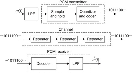
Despite all of these advantages, you need to remember that because of the sampling and the quantization the process used to obtain PCM signals is neither linear nor time invariant, and as such its analysis is complicated. Figure 12.9 shows a transmitter, a channel, and a receiver of a PCM system.
The main disadvantage of PCM is that its bandwidth is wider than that of the analog message it represents. This is due to the rectangular pulses in the signal. If we represent the PCM signal s(t) as

Suppose that the function is a sinc function having an infinite time support so that s(t) also has an infinite time support. If
Suppose you have a binary signal 01001001, with a duration of 8 units of time, and wish to represent it using rectangular pulses and sinc functions. Consider the bandwidth of each of the representations.
Solution
Using pulses φ(t), the digital signal can be expressed as

If the pulses are rectangular,
If this digital signal is transmitted and received without any distortion, at the receiver we can use the orthogonality of the φ(t) signals or sample the received signal at nTs to obtain the bn. Clearly, each of these pulses has disadvantages—the advantage of having a finite support in the time or in the frequency becomes a disadvantage in the other domain.
Baseband and Band-Pass Communication Systems
A baseband signal can be transmitted over a pair of wires (like in a telephone), coaxial cables, or optical fibers. But a baseband signal cannot be transmitted over a radio link or a satellite because this would require a large antenna to radiate the low-frequency spectrum of the signal. Thus, the signal spectrum must be shifted to a higher frequency by modulating a carrier by the baseband signal. This can be done by amplitude and by angle modulation (frequency and phase). Several forms are possible.
Suppose the binary signal 01001101 is to be transmitted over a radio link using AM and FM modulation. Discuss the different band-pass signals obtained.
Solution
The binary message can be represented as a sequence of pulses with different amplitudes. For instance, we could represent the binary digit 1 by a pulse of constant amplitude, and the binary 0 is represented by switching off the pulse (see the corresponding modulating signal m1(t) in Figures 12.10(a) and 12.10(b)). Another possible representation would be to represent the binary digit 1 with a positive pulse of constant amplitude, and 0 with the negative of the pulse used for 1 (see the corresponding modulating signal m2(t) in Figures 12.10(c) and 12.10(d)).

In AM modulation, if we use m1(t) to modulate a sinusoidal carrier cos(Ω0t) we obtain the amplitude-shift keying (ASK) signal shown in Figure 12.10(a). On the other hand, when using m2(t) to modulate the same carrier we obtain a phase-shift keying (PSK) signal shown in Figure 12.10(c). In this case, the phase of the carrier is shifted 180o as the pulse changes from positive to negative.
Using FM modulation, the symbol 0 is transmitted using a windowed cosine of some frequency Ωc0 and the symbol 1 is transmitted with a windowed cosine of frequency Ωc1 resulting in frequency-shift keying (FSK). The data are transmitted by varying the frequency. In this case it is possible to get the same modulated signals for both m1(t) and m2(t). The modulated signals are shown in Figure 12.10(b and d).
The ASK, PSK, and FSK are also known as BASK, BPSK, and BFSK, respectively, by adding the word “binary” (B) to the corresponding amplitude-, phase-, and frequency-shift keying.
12.4.2. Time-Division Multiplexing
In a telephone system, multiplexing enables multiple conversations to be carried across a single shared circuit. The first multiplexing system used was frequency-division multiplexing (FDM), which we covered in Chapter 6. In FDM an available bandwidth is divided among different users. In the case of voice communications, each user is allocated a bandwidth of 4 KHz, which provides good fidelity. In FDM, a user could use the allocated frequencies all of the time, but the user could not go outside the allocated band of frequencies.
Pulse-modulated signals have large bandwidths, and as such, when transmitted together they overlap in frequency, interfering with each other. However, these signals only provide information at each of the sampling times, so that one could insert in between these times other samples that will be separated at the receiver. This is the principle of time-division multiplexing (TDM), where pulses from different signals are interspersed into one signal and converted into a PCM signal and transmitted. See Figure 12.11. At the receiver, the signal is changed back into the pulse-modulated signal and separated into the number of signals interspersed at the input. Repeaters placed between the transmitter and the receiver regenerate a clean binary signal from a noisy binary signal along the way. The noisy signal coming into the repeater is thresholded to known binary levels and resent. A large part of the cost of a transmission facility is due to these repeaters that are placed about every mile along the line.

TDM allows the transmission of different types of data, and mixture of analog and digital using different multiplexing techniques. Not to lose information, the switch at the receiver needs to be synchronized with the switch at the transmitter. Frame synchronization consists in sending a synchronizing signal for each frame. An additional channel is allocated for this purpose. To accommodate more users, the width of the pulses used for each user needs to become narrower, which increases the overall bandwidth of the multiplexed signal.
12.4.3. Spread Spectrum and Orthogonal Frequency-Division Multiplexing
The objective of TDM is to put several users or different types of data together sharing the same bandwidth at different times. Likewise, FDM users share part of the available bandwidth all the time. TDM and FDM are examples of how to use bandwidth in an efficient way. In other situations, like in quadrature-amplitude modulation (QAM), the objective is to send two messages over the same bandwidth using the orthogonality of the carriers to recover them. In spread spectrum, the objective is to use the orthogonality of the carriers associated with different users to share the available spectrum, while spreading the message in frequency so that it occupies a bandwidth much larger than that of the message. On the other hand, orthogonal frequency-division multiplexing (OFDM) is a multicarrier system where the carriers are orthogonal.
Sharing the radio spectrum among users, or multiple access, is a basic strategy of wireless communication systems. Basic modalities are derived from FDM, TDM, and spread spectrum. In FDMA the spectrum is shared by assigning specific channels to users, permanently or temporarily. TDMA allows access to all of the available spectrum, but each user is assigned a time interval in which to access it. CDMA uses spread spectrum, where a user's message is spread or encrypted over the available spectrum using a code to differentiate the different users. The objective of these three techniques is to maximize the radio spectrum utilization.
Spread Spectrum—A Famous Actress Idea
Not surprisingly, the first mention of the use of frequency hopping, a form of spread spectrum, for secure communications came from a patent by Nikolas Tesla in 1903. As you recall, Tesla is the world-renowned Serbian-American inventor, and physicist, and mechanical and electrical engineer who pioneered amplitude modulation.
The most celebrated invention of frequency-hopping was, however, that of Hedy Lamarr and George Antheil, who in 1942 received a U.S. patent for their “secret communications system,” in which they used a piano-roll for frequency-hopping. This was during World War II, and their idea was to stop the enemy from detecting or jamming radio-guided torpedoes. To avoid the jammer, in frequency-hopping spread spectrum the transmitter changes in a quasi-random way the center frequency of the transmitted signal. Hedy Lamarr (1913–2000) was an Austrian-American actress and communications technology innovator, while George Antheil (1900–1959) was an American composer and pianist. Their patent was never applied, and it would be many years before the technology was actually deployed. Ms. Lamarr conceived the idea of hopping from frequency to frequency just as a piano player plays the same notes, but in different octaves. Their concept eventually provided the basis for the CDMA airlink, which Qualcomm commercialized in 1995. Today, CDMA and its core principles provide the backbone for wireless communications, thanks to the creative vision of an extraordinary woman 70, 74 and 62.
Spread Spectrum
A spread-spectrum system is one in which the transmitted signal is spread over a wide frequency band, much wider than the bandwidth required to transmit the message. Such a system would take a baseband voice signal with a bandwidth of a few kilohertz and spread it to a band of many megahertz. Two types of spread-spectrum systems are:
■ Direct-sequence system: A digital code sequence with a bit rate higher than the message is used to obtain the modulated signal.
■ Frequency-hopping system: The carrier frequency is shifted in discrete increments in a pattern dictated by a code sequence. We will not consider this here.
Direct-Sequence Spread-Spectrum
Suppose the message m(t) we wish to transmit is a polar binary signal, and that a spreading code c(t), also in polar binary form, is modulated by the message to obtain the modulated baseband signal
(12.21)
When transmitting over a radio link the baseband signal x(t) modulates an analog carrier to obtain the transmitting signal s(t). At the receiver, if no interference occurred in the transmission, the received signal r(t) = s(t), and after demodulation using the analog carrier frequency, the spread signal x(t) is obtained. If we multiply it by c(t) we get
(12.22)

Two significant advantages of direct-sequence spread spectrum are:
■ Robustness to noise and jammers: The above detection or despreading is idealized. The received signal will have interferences due to channel noise, interference from other users, and even, in military applications, intentional jamming. Jamming attempts to corrupt the sent message by adding to it either a narrowband or a wideband signal. If at the receiver, the spread signal contains additive noise η(t) and a jammer j(t), it is demodulated by the BPSK system. The received baseband signal is
(12.23)
Multiplying it by c(t) gives
(12.24)
■ Robustness to interference from other users: Assuming no noise or jammer, if the received baseband signal comes from two users—that is,
(12.25)
(12.26)
Simulation of direct sequence spread spectrum.
In this simulation we consider that the message is randomly generated and that the spreading code is also randomly generated (our code does not have the same characteristics as the one used to generate the code for spread-spectrum systems). To generate the train of pulses for the message and the code we use filters of different length (recall the spreading code changes more frequently than the message). The spreading makes the transmitting signal have a wider spectrum than that of the message (see Figure 12.13).

The binary transmitting signal modulates a sinusoidal carrier of frequency 100 Hz. Assuming the communication channel does not change the transmitted signal and perfect synchronization at the analog receiver is possible, the despread signal coincides with the sent message. In practice, the effects of multipath in the channel, noise, and possible jamming would not make this possible.
%%%%%%%%%%%%%%%%
% Simulation of
% spread spectrum
%%%%%%%%%%%%%%%%
clear all; clf
% message
m1 = rand(1,12)>0.9;m1 = (m1-0.5) ∗ 2;
m = zeros(1,00);
m(1:9:100) = m1
h = ones(1,9);
m = filter(h,1,m);
% spreading code
c1 = rand(1,25)>0.5;c1 = (c1-0.5) ∗ 2;
c = zeros(1,100);
c(1:4:100) = c1;
h1 = ones(1,4);
c = filter(h1,1,c);
Ts = 0.0001; t = [0:99] ∗ Ts;
s = m. ∗ c;
figure(1)
bar(t,m); axis([0 max(t) -1.2 1.2]);grid; ylabel(‘m(t)’)
subplot(312)
bar(t,c); axis([0 max(t) -1.2 1.2]);grid; ylabel(‘c(t)’)
subplot(313)
bar(t,s); axis([0 max(t) -1.2 1.2]);grid; ylabel(‘s(t)’); xlabel(‘t (sec)’)
% spectrum of message and spread signal
M = fftshift(abs(fft(m)));
S = fftshift(abs(fft(s)));
N = length(M);K = [0:N-1];w = 2 ∗ K ∗ pi/N-pi; f = w/(2 ∗ pi ∗ Ts);
figure(2)
subplot(211)
subplot(212)
plot(f,S); grid; axis([min(f) max(f) 0 1.1 ∗ max(S)]);ylabel(‘—S(f)—’); xlabel(‘f (Hz)’)
% analog modulation and demodulation
s = s. ∗ cos(200 ∗ pi ∗ t);
r = s. ∗ cos(200 ∗ pi ∗ t);
% despreading
mm = r. ∗ c;
for k = 1:length(mm);
if mm(k) > 0
m2(k) = 1;
else
m2(k) = -1;
end
end
figure(3)
subplot(411)
plot(t,s); axis([0 max(t) 1.1 ∗ min(s) 1.1 ∗ max(s)]);grid; ylabel(‘s_a(t)’)
subplot(412)
plot(t,r); axis([0 max(t) 1.1 ∗ min(r) 1.1 ∗ max(r)]);grid; ylabel(‘r(t)’)
subplot(413)
plot(t,mm); axis([0 max(t) 1.1 ∗ min(mm) 1.1 ∗ max(mm)]);grid; ylabel(‘m_a(t)’)
subplot(414)
bar(t,m2); axis([0 max(t) -1.2 1.2]);axis([0 max(t) 1.1 ∗ min(mm) 1.1 ∗ max(mm)])
grid;ylabel(‘m(t)’); xlabel(‘t (sec)’)
Orthogonal Frequency-Division Multiplexing
OFDM is a multicarrier modulation technique where the available bandwidth is divided into narrowband subchannels. It is used for high data-rate transmission over mobile wireless channels 27, 60 and 4.
If {dk, k = 0, …, N − 1} are symbols to be transmitted, the OFDM-modulated signal is
(12.27)


OFDM Implementation with FFT
If the modulated signal s(t), 0 ≤ t ≤ T, in Equation (12.27) is sampled at t = nT/N, we obtain for a frame the inverse DFT
(12.28)

Figure 12.14 gives a general description of the transmitter and receiver in an OFDM system: The high-speed data in binary form coming into the system are transformed from serial to parallel and fed into an IFFT block giving as output the transmitting signal that is sent to the channel. The received signal is then fed into an FFT block providing estimates of the sent symbols that are finally put in serial form.

12.5. What Have We Accomplished? Where Do We Go from Here?
In this chapter we have seen how the theoretical results presented in the third part of the book relate to digital signal processing, digital control, and digital communications. The Fast Fourier Transform made possible the establishment and significant growth of digital signal processing as a technical area. The next step for you could be to get into more depth in the theory and applications of digital signal processing, preferably including some theory of random variables and processes, toward statistical signal processing, speech, and image processing. We have shown you also the connection of the discrete-time signals and systems with digital control and communications. Deeper understanding of these areas would be an interesting next step. You have come a long way, but there is more to learn.
..................Content has been hidden....................
You can't read the all page of ebook, please click here login for view all page.