
12
Frequency Domain Representation
Chapter Outline
In this chapter we are going to examine the DFT (Discrete Fourier Transform) and its more popular cousin, the FFT (Fast Fourier Transform). The FFT is used in many applications, and we will see its uses in broadcast modulation and distribution systems. It also lays the basis for the DCT (Discrete Cosine Transform), commonly used in image compression, which is also covered.
This chapter has more mathematics than most of the others in this book. It requires some familiarity with basic trigonometry, complex numbers and the complex exponential. A refresher on these topics is provided as an appendix for those who haven’t used these in a long time.
The DFT is simply a transform. It takes a sequence of sampled data (a signal), and computes the frequency content of that sampled data sequence. This will give the representation of the signal in the frequency domain, as opposed to the familiar time domain representation. This can be done in both the vertical and horizontal dimensions, although for now we will assume a one-dimensional signal. The result is a frequency-domain representation of the signal, providing the spectral content of a given signal. All of the signal information is preserved, but in a different form.
The IDFT (Inverse Discrete Fourier Transform) computes the time-domain representation of the signal from the frequency-domain information. Using these transforms, it is possible to switch between the time domain signal and the frequency domain spectral representation. The DFT takes a complex signal and decomposes it into a sum of different frequency cosine and sine waves.
In order to appreciate what is happening, we are going to examine a few simple examples. This will involve multiplying and summing up complex numbers, which, while not difficult, can be tedious. We will minimize the tedium by using a short transform length, but it cannot really be avoided in order to understand the DFT.
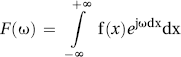
We will start with the definition of the Fourier transform. The basic Fourier theory tells us that any signal can be represented at a sum of various frequency components, with a particular gain and phase for each component. The signal, f(x), is multiplied and integrated by each possible frequency. Each frequency is represented by the complex exponential, which is just a complex sinusoid. This is also known as the Euler equation:
![]()
The Fourier transform is defined as:
Let’s see if we can start simplifying: we will decide to perform the calculation over a finite length of sampled data signal “x”, which contains N samples, rather than continuous signal f(x) Ci. This gets rid of the infinity, and makes this something we can actually build.
![]()
Note that ω is a continuous variable, which we evaluated over a 2π interval, usually from −π to π. Now we will be transforming a sampled time-domain signal to a sampled frequency-domain spectral plot. So rather than computing ω continuously from −π to π, we will instead compute ω at M equally spaced points over an interval of 2π. To avoid aliasing in the frequency domain, we must make M ≥ N. The reverse transform is the IDFT (or IFFT), which reconstructs the sampled time-domain signal of length N and does not require more than N points in the frequency domain. Therefore we will set N = M, and the frequency domain representation will have the same number of points as the time domain representation. We will use the convention “xi” to represent the time-domain version of the signal, and “Xk” to represent the frequency-domain representation of the signal. Both indexes i and k will run from 0 to N−1.
12.1 DFT and IDFT Equations
DFT (time → frequency)
![]()
IDFT (frequency → time)
![]()
These equations do appear very similar. The differences are the negative sign on the exponent on the DFT equation, and the factor of 1 / N on the IDFT equation. The DFT equation requires that every single sample in the frequency domain has a contribution from each and every one of the time domain samples. And the IDFT equation requires that every single sample in the time domain has a contribution from each and every one of the frequency domain samples. To compute a single sample of either transform requires N complex multiplies and additions. To compute the entire transform will require computing N samples, for a total of N2 multiplies and additions. This can become a computational problem when N becomes large. As we will see later, this is the reason the FFT and IFFT were developed.
The values of Xk represent the amount of signal energy at each frequency point. Imagine taking a spectrum of 1 MHz which we divide into N bins. If N = 20, then we will have 20 frequency bins, each 50 kHz wide. The DFT output, Xk, will represent the signal energy in each of these bins. For example, X0 will represent the signal energy at 0 kHz, or the DC component of the signal. X1 will represent the frequency content of the signal at 50 kHz. X2 will represent the frequency content of the signal at 100 kHz. X19 will represent the frequency content of the signal at 950 kHz.
A few comments on these transforms might prove helpful. Firstly, they are reversible. We can take a signal represented by N samples, and perform the DFT on it. We will get N outputs representing the frequency response or spectrum on the signal. If we take this frequency response and perform the IDFT on it, we will get back our original signal of N samples back. Secondly, when the DFT output gives the frequency content of the input signal, it is assuming that the input signal is periodic in N. To put it another way, the frequency response is actually the frequency response of an infinite long periodic signal, where the N long sequence of xi samples repeat over and over. Lastly, the input signal xi is usually assumed to be a complex (real and quadrature) signal. The frequency response samples Xk are also complex. Often we are more interested in only the magnitude of the frequency response Xk, which can be more easily displayed. But in order to get back the original complex input xi using the IDFT, we would need the complex sequence Xk.
At this point, we will do a few examples, selecting N = 8.
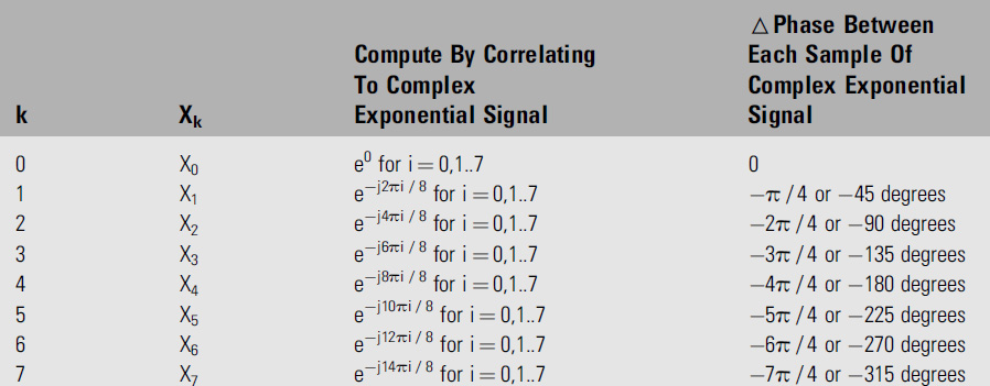
For our N = 8 point DFT, the output gives us the distribution of input signal energy into eight frequency bins, corresponding to the frequencies in Table 12.1 below. By computing the DFT coefficients Xk, we are performing a correlation, or trying to match, our input signal to each of these frequencies. The magnitude DFT output coefficients Xk represent the degree of match of the time-domain signal xi to each frequency component.
Table 12.1
12.1.1 First DFT Example
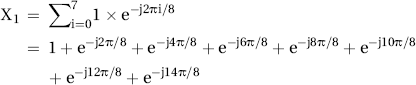
Let’s start with a simple time domain signal consisting of {1,1,1,1,1,1,1,1}. Remember, the DFT assumes this signal keeps repeating, so the frequency output will actually be that of an indefinite string of 1s. As this signal is unchanging, then by intuition, we will expect that zero frequency component (DC of signal) is going to be the only non-zero component of the DFT output Xk.
Starting with ![]() and setting N = 8 and all xi = 1:
and setting N = 8 and all xi = 1:
![]() , and setting k=0 (recall that e0=1)
, and setting k=0 (recall that e0=1)
![]()
Next, evaluate for k = 1:
![]()
X1 = 0
The eight terms of the summation for X1 cancel out. This makes sense because it’s a sum of eight equally spaced points about the origin on the unit circle of the complex plane. The summation of these points must equal the center, in this case zero.
Next, evaluate for k = 2:

![]()
We will find out similarly that X3, X4, X5, X6, X7 are also zero. Each of these will represent eight points equally spaced about the unit circle. X1 has its points spaced at −45° increments, X2 has its points spaced at −90° increments, X3 has its points spaced at −135° increments, and so forth (the points may wrap multiple times around the unit circle in the frequency domain). So, as we expected, the only non-zero term is X0, which is the DC term. There is no other frequency content of the signal.
Now, let us use the IDFT to get the original sequence back:

![]()
Since X0 = 8 and the rest are zero, we only need to evaluate the summation for k = 0:
![]()
This is true for all values of i (the 0 in the exponent means the value of “i” is irrelevant). So we get an infinite sequence of 1s.
In general however, we would evaluate for i from 0 to N−1. Due to the periodicity of the transform, there is no point in evaluating when i = N or greater. If we evaluate for i = N, we will find we get the same value as i = 0, and for i = N + 1, we will get the same value as i = 1.
12.1.2 Second DFT Example
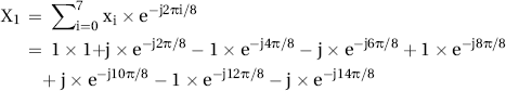
Let’s consider another simple example, with a time domain signal {1,j,−1,−j,1,j,−1,−j}. This is actually the complex exponential ![]() . This signal consists of a single frequency, and corresponds to one of the frequency “bins” that the DFT will measure. So we can expect a non-zero DFT output in this frequency bin, but zero elsewhere. Let’s see how this works out.
. This signal consists of a single frequency, and corresponds to one of the frequency “bins” that the DFT will measure. So we can expect a non-zero DFT output in this frequency bin, but zero elsewhere. Let’s see how this works out.
Starting with ![]() and setting N = 8 and xi = {1,j,−1,−j,1,j,−1,−j}:
and setting N = 8 and xi = {1,j,−1,−j,1,j,−1,−j}:
![]()
![]() , so the signal has no DC content, as expected. Notice that to calculate X0 – which is the DC content of xI – the DFT just sums (essentially averaging) the input samples.
, so the signal has no DC content, as expected. Notice that to calculate X0 – which is the DC content of xI – the DFT just sums (essentially averaging) the input samples.
Next, evaluate for k = 1:
![]()
![]()
If you take the time to work this out, you will see that all eight terms of the summation cancel out. This also happens for X3, X4, X5, X6, and X7. Let’s look at X2 now. We will also express xi using complex exponential format of ![]() .
.
![]()

Remember that when exponentials are multiplied the exponents are added (x2 × x3 = x5). Here the exponents are identical, except of opposite sign, so they add to zero.
![]()
The sole frequency component of the input signal is X2 because our input is a complex exponential frequency at the exact frequency that X2 represents.
12.1.3 Third DFT Example
Next, we can try modifying xi such that we introduce a phase shift, or delay (like substituting a sine wave for a cosine wave). If we introduce a delay, so xi starts at j instead of 1, but is still the same frequency, the input xi is still rotating around the complex plane at the same rate, but starts at j (angle of π / 2) rather than 1 (angle of 0). Now the sequence xi = {j,−1,−j,1,j,−1,−j,1} or ![]() .
.
The DFT output will result in X0, X1, X3, X4, X5, X6, and X7 = 0, as before. Changing the phase cannot cause any new frequency to appear in the other bins.
Next, evaluate for k = 2:
![]()
![]()
We need to sum the two values of the two exponents:
![]()
Substituting back this exponent value:
![]()
So we get exactly the same magnitude at the frequency component X2. The difference is the phase of X2. Therefore we can see that the DFT does not just pick out the frequency components of a signal, but is sensitive to the phase of those components. The phase, as well as amplitude of the frequency components Xk, can be represented because the DFT output is complex.
The process of the DFT is to correlate the N sample input data stream xi against N equally spaced complex frequencies. If the input data stream is one of these N complex frequencies, then we will get a perfect match, and get zero in the other N−1 frequencies which don’t match. But what happens if we have an input data stream with a frequency in between one of the N frequencies?
To review, we have looked at three simple examples. The first was a constant level signal, so the DFT output was just the zero frequency or DC component. The second example was a complex frequency which matched exactly to one of the frequency bins, Xk, of the DFT. The third was the same complex frequency, but with a phase offset. The fourth will be a complex frequency not matched to one of the N frequencies used by the DFT.
12.1.4 Fourth DFT Example
We will look at an input signal of frequency e+j2.1πi / 8. This is rather close to e+j2πi / 8, so we would expect a rather strong output at X1. Let’s see what the N = 8 DFT result is – hopefully the arithmetic is all correct. Slogging through this arithmetic is purely optional – the details are shown to provide a complete example.
Generic DFT equation for N = 8:![]()


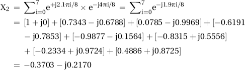
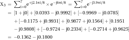
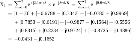

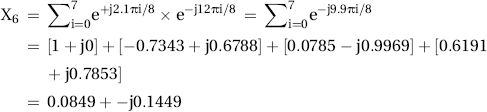

That was a bit tedious, but there is some insight to be gained from the results of these simple examples.
Table 12.2 shows how the DFT is able to represent the signal energy in each frequency bin. The first example has all the energy at DC. The second and third examples are complex exponentials at frequency ω = π / 2 radians/sample, which corresponds to DFT output X2. The magnitude of the DFT outputs is the same for both examples, since the only difference of the inputs is the phase. The fourth example is the most interesting. In this case, the input frequency is close to π / 4 radians/sample, which corresponds to DFT output X1. So X1 does capture most of the energy of the signal. But small amounts of energy spill into other frequency bins, particularly the adjacent bins.
Table 12.2

We can increase the frequency sorting ability of the DFT by increasing the value of N. This will narrow each frequency bin because the frequency spectrum is divided into N sections in the DFT. This will result in a given frequency component being more selectively represented by a particular frequency bin. For example, the frequency response plots of the filters contained in the FIR chapter are computed with a value of N equal to 1024. This means the spectrum was divided into 1024 sections, and the response computed for each particular frequency. When plotted together, this gives a very good representation of the complete frequency spectrum.
Please note this also requires taking a longer input sample stream xi , equal to N. This, in turn, will require a much greater number of operations to compute.
12.2 Fast Fourier Transform
At some point, some smart people searched for a way to compute the DFT in a more efficient way. The result is the FFT, or Fast Fourier Transform. Rather than requiring N2 complex multiplies and additions, the FFT requires N × log2N complex multiplies and additions. This may not sound like a big deal, but look at the comparison in Table 12.3 below.
Table 12.3

So by using the FFT algorithm on a 1024 point (or sample) input, we are able to reduce the computational requirements to less than 1%, or by two orders of magnitude.
The FFT achieves this by reusing previously calculated interim products. We can see this through a simple example.
Let’s start with the calculation of the simplest DFT : N = 2 DFT.
Generic DFT equation for ![]()
![]()
![]()
As e0 = 1, we can simplify to find:
![]()
![]()
Next, we will do the four point (N = 4) DFT.
![]()
![]()
![]()
![]()
The term ![]() repeats itself with a period of k = 4, as the complex exponential makes a complete circle and begins another. This periodicity means that
repeats itself with a period of k = 4, as the complex exponential makes a complete circle and begins another. This periodicity means that ![]() is equal when evaluated for k = 0, 4, 8, 12… It is again equal for k = 1, 5, 9, 13… Because of this, we can simplify the last two terms of expressions for X2 and X3 (shown in bold below). We can also remove the exponential when it is to the power of zero.
is equal when evaluated for k = 0, 4, 8, 12… It is again equal for k = 1, 5, 9, 13… Because of this, we can simplify the last two terms of expressions for X2 and X3 (shown in bold below). We can also remove the exponential when it is to the power of zero.
![]()
![]()
![]()
![]()
Now we are going to rearrange the terms of the four point (N = 4) DFT, grouping the even and odd terms together.
![]()
![]()
![]()
![]()
Next we will factor x1 and x3 to get this particular form:
![]()


Here is the result:
![]()
![]()
![]()
![]()
Now comes the insightful part. Comparing the four equations above, you can see that the bracketed terms used for X0 and X1 are also present in X2 and X3. So we don’t need to recompute these terms during the calculation of X2 and X3. We can simply multiply them by the additional exponential outside the brackets. This reusing of partial products in multiple calculations is the key to understanding the FFT efficiency, so at the risk of being repetitive, this is shown again more explicitly below.
→ define ![]()
![]()
→ define ![]()
![]()
![]()
![]()
This process quickly gets out of hand for anything larger than a four point (N = 4) FFT. So we are going to use a type of representation called a flow graph, shown in Figure 12.1 below.

Figure 12.1 FFT flow graph.
The flow graph is an equivalent way of representing the equations, and moreover, represents the actual organization of the computations. You can check the simple example above to see the flow graph gives the same results as the DFT equations. For example, X0 = x0 + x1 + x2 + x3, and by examining the flow graph, it is apparent that X0 = A + B = [x0 + x2] + [x1 + x3], which is the same result. The order of computations would be to compute pairs {A, C} and {B, D} in the first stage. The next stage would be to compute {X0, X2} and {X1, X3}.
These stages (our example above has two stages) are composed of “butterflies”. Each butterfly has two complex inputs and two complex outputs. The butterfly involves one or two complex multiplications and two complex additions. In the first stage, there are two butterflies to compute the two pairs {A, C} and {B, D}. In the second stage, there are two butterflies to compute the two pairs {X0, X2} and {X1, X3}. The complex exponentials multiplying the data path are known as “twiddle factors”. In higher N count FFTs, they are simply sine and cosine values that are usually stored in a table.
Now we can see why the FFT is effective in reducing the number of computations. Each time the FFT doubles in size (N increases by a factor of two), we need to add one more stage. Thus, a four-point FFT requires two stages; an eight point FFT requires three stages and a 16 point FFT requires four stages, and so on. The amount of computations required for each stage is proportional to N. The required number of stages is equal to log2 N. Therefore, the FFT computational load increases by N × log2 N. The DFT computational load increases as N2.
This is also the reason why FFT sizes are almost always in powers of 2 (2, 4, 8, 16, 32, 64..). This is sometimes called a “radix 2” FFT. So rather than a 1000 point FFT, one will see a 1024 point FFT. In practice, this common restriction to powers of two is not a problem.
12.3 Discrete Cosine Transform
Next, we will discuss the Discrete Cosine Transform, or DCT. Until now we have been talking about the DFT or FFT operating on one-dimensional signals, which are often complex (may have real and quadrature components). The DCT is usually used for two-dimensional signals, such as an image presented by a rectangular array of pixels, and which is a real signal only. When we discuss frequency, it will be in the context of how rapidly the sample values change. We will be sampling spatially across the image in either the vertical or horizontal direction with the DCT.
The DCT is usually applied across an N by N array of pixel data. For example, if we take a region composed of eight by eight pixels, or 64 pixels total, we can transform this into a set of 64 DCT coefficients, which is the spatial frequency representation of the eight by eight region of the image. This is very similar to the DCT. However, instead of expressing the signal as a combination of the complex exponentials of various frequencies, we will be expressing the image data as a combination of cosines of various frequencies, in both vertical and horizontal dimensions.
DFT representation is for a periodic signal, or one that is assumed to be periodic. Imagine connecting a series of identical signals together, end to end. Where the end of the sequence connects to the beginning of the next, there will be a discontinuity, or a step function. This will represent high frequency.
For the DCT, we make an assumption that the signal is folded over on itself. So an eight-long signal depicted becomes 16-long when appended as flipped. This 16-long signal is then symmetric about the midpoint. This is the same property of cosine waves. A cosine is symmetric about the midpoint, which is at π (since the period is from 0 to 2π). This property is preserved for higher frequency cosines, as shown by the figures below, showing the sampled cosine waves. The waveform is eight samples long, and if folded over will create a 16-long sampled waveform which will be symmetric, start and end with the same value and has “u” cycles across the 16 samples.
To continue requires explanation of some terminology. The value of a pixel at row x and column y is designated as f(x, y), as shown in Figure 12.3. We will compute the DCT coefficients, F(u, v) using equations which will correlate the pixels to the vertical and horizontal cosine frequencies. In the equations, “u” and “v” correspond to both the indices in the DCT array, and the cosine frequencies as shown in Figure 12.3.
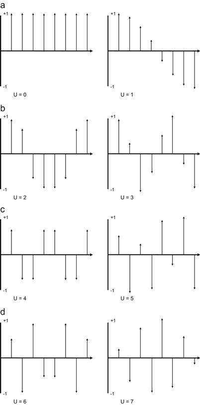
Figure 12.2a–12.2d Sample cosine frequencies used in DCT.
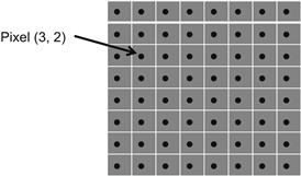
Figure 12.3 Block of pixels used to compute DCT.
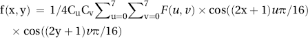
The relationship is given in the DCT equation, shown below for the eight by eight size.

where
![]()
![]()
f(x,y) = the pixel value at that location
This represents 64 different equations, for each combination of u, v. For example:
![]()
Simply put, the summation of all 64 pixel values divided by eight. F(0, 0) is the DC level of the pixel block.

The nested summations indicate that for each of the 64 DCT coefficients, we need to perform 64 summations. This requires 64 × 64 = 4096 calculations, which is very process intensive.
The DCT is a reversible transform (provided enough numerical precision is used), and the pixels can be recovered from the DCT coefficients as shown below:
![]()
![]()
Another way to look at the DCT is through the concept of basis functions.
The tiles represent the video pixel block for each DCT coefficient. If F(0, 0) is non-zero, and the rest of the DCT coefficients equal zero, the video will appear as the {0, 0} tile in Figure 12.4. This particular tile is a constant value in all 64 pixel locations, which is what is expected since all the DCT coefficients with some cosine frequency content are zero.

Figure 12.4 DCT basis functions.
If F(7, 7) is non-zero, and the rest of the DCT coefficients equal zero, the video will appear as the {7, 7} tile in Figure 12.4, which shows high frequency content in both vertical and horizontal direction. The idea is that any block of eight by eight pixels, no matter what the image, can be represented as the weighted sum of these 64 tiles in Figure 12.4.
The DCT coefficients, and the video tiles they represent, form a set of basis functions. From linear algebra, any set of function values f(x,y) can be represented as a linear combination of the basis functions.
The whole purpose of this is to provide an alternate representation of any set of pixels, using the DCT basis functions. By itself, this exchanges one set of 64 pixel values with a set of 64 DCT values. However, in many image blocks many of the DCT values are near zero, or small, and can be presented with few bits. This can allow the pixel block to be presented more efficiently with fewer values. However, this representation is approximate, because when we minimize the bits representing various DCT coefficients, we are quantizing. This is a loss of information, meaning the pixel block cannot be restored perfectly.
abcd