
14
Video Compression Fundamentals
Chapter Outline
MPEG is often considered synonymous with image compression. MPEG stands for Moving Pictures Experts Group, a committee that publishes international standards on video compression. MPEG is a portfolio of video compression standards, which will be discussed further in the next chapter.
Image compression theory and implementation focuses on taking advantage of the spatial redundancy present in the image. Video is composed of a series of images, usually referred to as frames, and so can be compressed by compressing the individual frames as discussed in the last chapter. However, there are temporal (or across time) redundancies present across video frames: the frame immediately following has a lot in common with the current and previous frames. In most videos there will be a significant amount of repetition in the sequences of frames. This property can be used to reduce the amount of data used to represent and store a video sequence. In order to take advantage of the temporal redundancy, this commonality must be determined across the frames.
This is known as predictive coding, and is effective in reducing the amount of data that must be stored or streamed for a given video sequence. Usually only part of an image changes from frame to frame, which permits prediction from previous frames. Motion compensation is used in the predictive process. If an image sequence contains moving objects, then the motion of these objects within the scene can be measured, and the information used to predict the location of the object in frames later in the sequence.
Unfortunately, this is not as simple as just comparing regions in one frame to another. If the background is constant, and objects move in the foreground, there will be significant unchanging areas of the frames. But, if the camera is panning across a scene, there will be areas of subsequent frames that are the same, but will have shifted location from frame to frame. One way to measure this is to sum up all the absolute differences (without regard to sign), pixel by pixel, between two frames. Then the frame can be offset by one or more pixels, and the same comparison run. After many such comparisons, the sum of differences in the results can be compared, where the minimum result corresponds to the best match, and provides the basis for a method to determine the location offset of the match between frames. This is known as the minimum absolute differences (MAD) method, or sometimes it’s referred to as sum of absolute differences (SAD).
An alternative is the minimum mean square error (MMSE) method, which measures the sum of the squared pixel differences. This method can be useful because it accentuates large differences, due to the squaring, but the trade-off is the requirement for multiplies as well as subtractions.
14.1 Block Size
A practical trade-off has to be made when determining the block size (or macroblock) over which the comparison is run. If the block size is too small there is no benefit in trying to reuse pixel data from a previous frame rather than just use the current frame data. If the block is too large, many more differences will be likely, and it is difficult to get a close match. One obvious block size to run comparisons across would be the 8 × 8 block size used for DCT. Experimentation has shown that a 16 × 16 pixel area works well, and this is commonly used.
The computational efforts of running these comparisons can be enormous. For each macroblock, 256 pixels must be compared against a 16 × 16 area of the previous frame. If we assume the macroblock data could shift by up to, for example, 256 pixels horizontally or 128 pixels vertically (a portion of an HD 1080 × 1920) from one frame to another, there will be 256 possible shifts to each side, and 128 possible shifts up or down. This is a total of 512 × 256 = 131,072 permutations to check, each requiring 256 difference computations. This is over 33 million per macroblock, with 1080 / 16 × 1920/16 = 8100 macroblocks per HD image or frame.

Figure 14.1a – 14.1c Macroblock matching across nearby frames.
14.2 Motion Estimation
Happily, there are techniques to reduce this brute force method. A larger block size can be used initially, over larger portions of the image, to estimate the motion trend between frames. For example, we can enlarge the block size used for motion estimation to include macrocells on all sides, for a 48 × 48 pixel region. Once the motion estimation is completed, this can be used to dramatically narrow down the number of permutations to perform the MAD or MMSE over. This motion estimation process is normally performed using luminary (Y) data and performed locally for each region. In the case of the camera panning, large portions of an image with a common motion vector will move, but in cases with moving objects within the video sequence, different objects or regions will have different motion vectors.
Note that these motion estimation issues are present only on the encoder side. The decoder side is much simpler, as it must recreate the image frames based upon data supplied in compressed form. This asymmetry is common in audio, image, video or general data compression algorithms. The encoder must search for the redundancy present in the input data using some iterative method, whereas the decoder does not require this functionality.
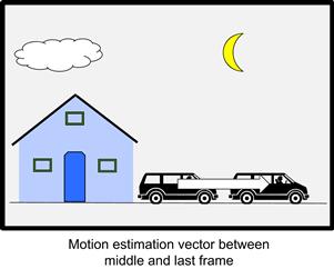
Figure 14.2 Motion estimation.
Once a good match is found, the macroblocks in the following frame data can be minimized during compression by referencing the macroblocks in previous frames. However, even a “good” match will have some error. These errors are referred to as residuals, or residual artifacts. These artifacts can be determined by differences in the four 8 ×8 DCTs in the macroblock and then coded and compressed as part of the frame data. Of course, if the residual is too large, coding the residual might require more data compared to just compressing the image data without any reference to the previous frame.
To begin MPEG compression, the source video is first converted to 4:2:0 format, so the chrominance data frame is one fourth the number of pixels – ½ vertical and ½ horizontal resolution. The video must be in progressive mode: each frame is composed of pixels from the same time instant (i.e. not interlaced).
At this point, a bit of terminology and hierarchy used in video compression needs to be introduced:
A pixel block refers to an 8 × 8 array in a frame.
A macrocell is 4 blocks, making a 16 × 16 array in a frame.
A slice is a sequence of adjacent macrocells in a frame. If data is corrupted, the decoding can typically begin again at the next slice boundary.
A group of pictures (GOP) is from one to several frames. The significance of the GOP is that it is self-contained for compression purposes. No frame within one GOP uses data from a frame in another GOP for compression or decompression. Therefore, each GOP must begin with an I-frame (defined below).
Most video compression algorithms have three types of frames:
I-frames – These are intra-coded frames – they are compressed using only information in the current frame. A GOP always begins with an I-frame, and no previous frame information is required to compress or decompress an I-frame.
P-frames – These are predicted frames. P-frames are compressed using image data from an I- or P-frame (that may not be the immediately preceding frame) when compared to the current P-frame. Restoring or decompressing the frame requires compressed data from a previous I- or P-frame, and residual data and motion estimation corresponding to the current P-frame are used. The video compression term for this is inter-coded, meaning the coding uses information across multiple video frames.
B-frames – These are bi-directional frames. B-frames are compressed using image data from preceding and successive I- or P-frames. This is compared to the current B data to form the motion estimation and residuals. Restoring or decompressing the B-frame requires compressed data from preceding and successive I- or P-frames, plus residual data and motion estimation corresponding to the current B-frame. B-frames are inter-coded.

Figure 14.3 Group of pictures (GOP) example.
By finishing the GOP with a P-frame, the last few B-frames can be decoded without needing information from the I-frame of the following GOP.
14.3 Frame Processing Order
The order of frame encode processing is not sequential. Forward and backward prediction means that each frame has a specific dependency mandating the processing order, and requires buffering of the video frames to allow out-of-sequential order processing. This also introduces multi-frame latency in the encoding and decoding process.
At the start of the GOP, the I-frame is processed first. Then the next P-frame is processed, as it needs the current frame plus information from the previous I- or P-frame. Then the B-frames in between are processed, as, in addition to the current frame, information from both previous and post frames are used. Then the next P-frame, and after that the intervening B-frames, as shown in the processing order given in Figure 14.4.

Figure 14.4 Video frame sequencing example.
Note that since this GOP begins with an I-frame and finishes with a P-frame, it is completely self-contained, which is advantageous when there is data corruption during playback or decoding. A given corrupted frame can only impact one GOP. The following GOP, since it begins with an I-frame, is independent of problems in a previous GOP.
14.4 Compressing I-frames
I-frames are compressed in very similar fashion to the JPEG techniques covered in the last chapter. The DCT is used to transform pixel blocks into the frequency domain, after which quantization and entropy coding is performed. I-frames do not use information in any other video frame, therefore an I-frame is compressed and decompressed independently from other frames. Both the luminance and chrominance are compressed, separately. Since the 4:2:0 format is used, the chrominance will have only ¼ of the macrocells compared to the luminance. The quantization table (14.1) used is given below. Once more, notice how larger amounts of quantization are used for higher horizontal and vertical frequencies, as human vision is less sensitive to high frequency.
Luminance and Chrominance Quantization Table

Further scaling is provided by a quantization scale factor, which will be discussed further in the rate control description section.
The DC coefficients are coded differentially, using the difference from the previous frame, which takes account of the high degree of the average, or DC, level of adjacent blocks. Entropy encoding similar to JPEG is used. In fact, if all the frames are treated as I-frames, this is pretty much the equivalent of JPEG compressing each frame of image independently.
14.5 Compressing P-frames
When processing P-frames, a decision needs to be made for each macroblock, based upon the motion estimation results. If the search for a match with another macroblock does not yield a good match in the previous I- or P-frame, then it must be coded as I-frames are coded – no temporal redundancy can be taken advantage of. However, if a good match is found in the previous I- or P-frame, then the current macroblock can be represented by a motion vector to the matching location in the previous frame, and by computing the residual, quantizing and encoding (inter-coded). The residual uses a uniform quantizer, and this quantizer treats the DC component the same as the rest of the AC coefficients.
Residual Quantization Table

Some encoders also compare the number of bits used to encode the motion vector and residual to ensure there is a saving when using the predictive representation. Otherwise, the macroblock can be intra-coded.
14.6 Compressing B-frames
B-frames try to find a match using both preceding and following I- or P-frames for each macroblock. The encoder searches for a motion vector resulting in a good match over both the previous and following I- or P-frame, and if found uses that frame to inter-code the macroblock. If unsuccessful, then the macroblock must be intra-coded. Another option is to use the motion vector – but with both preceding and following frames simultaneously. When computing the residual, the B macroframe pixels are subtracted to the average of the macroblocks in the two I- or P-frames. This is done for each pixel, to compute the 256 residuals, which are then quantized and encoded.
Many encoders then compare the number of bits used to encode the motion vector and residual using the preceding, following, or average of both frames to see which provides the most bit savings with predictive representation. Otherwise, the macroblock is intra-coded.
14.7 Rate Control and Buffering
Video rate control is an important part of image compression. The decoder has a video buffer of fixed size, and the encoding process must ensure that this buffer never under- or overruns the buffer size, as either of these events can cause noticeable discontinuities for the viewer.
The video compression and decompression process requires processing of the frames in a non-sequential order. Normally, this is done in real-time. Consider these three scenarios:
Video storage – video frames arriving at 30 frames per minute must be compressed (encoded) and stored to a file.
Video readback – a compressed video file is decompressed (decoded), producing 30 video frames per minute.
Streaming video – a video source at 30 frames per minute must be compressed (encoded) to transmit over a bandwidth-limited channel (only able to support a maximum number of bits/second throughput). The decompressed (decoded) video is to be displayed at 30 frames per minute at the destination.
All of these scenarios will require buffering, or temporary storage of video files during the encoding and decoding process. As mentioned above, this is due to the out-of-order processing of the video frames. The larger the GOP, containing longer sequences of I-, P- and B-frames, the more buffering is potentially needed.
The number of bits needed to encode a given frame depends upon the video content. A video frame with lots of constant background (the sky, a concrete wall) will take few bits to encode, whereas a complex static scene like a nature film will require many more bits. Fast moving, blurring scenes with a lot of camera panning will be somewhere in-between as the quantizing of the high frequency DCT coefficients will tend to keep the number of bits moderate.
I-frames take the most bits to represent, as there are no temporal redundancy benefits. P-frames take fewer bits, and the least bits are needed for B-frames, as B-frames can leverage motion vectors and predictions from both previous and following frames. P and B-frames will require far fewer bits than I-frames if there is little temporal difference between successive frames, or conversely, may not be able to save any bits through motion estimation and vectors if the successive frames exhibit little temporal correlation.
Despite this, the average rate of the compressed video stream often needs to be held constant. The transmission channel carrying the compressed video signal may have a fixed bit-rate, and keeping this bit-rate low is the reason for compression in the first place. This does not mean the bits for each frame, for example at a 30 Hz rate, will be equal, but that the average bit rate over a reasonable number of frames may need to be constant. This requires a buffer, to absorb higher numbers of bits from some frames, and provide enough bits to transmit for those frames encoded with few bits.
14.8 Quantization Scale Factor
Since the video content cannot be predicted in advance, and this content will require a variable amount of bits to encode the video sequence, provision is made to dynamically force a reduction in the number of bits per frame. A scale factor is applied to the quantization process of the AC coefficients of the DCT, which is referred to as Mquant.
The AC coefficients are first multiplied by eight, then divided by the value in the quantization table, and then divided again by Mquant. Mquant can vary from 1 to 31, with a default value of eight. For the default level, Mquant just cancels the initial multiplication of eight.
One extreme is an Mquant of one. In this case, all AC coefficients are multiplied by 8, then divided by the quantization table value. The results will tend to be larger, non-zero numbers, which will preserve more frequency information at the expense of using more bits to encode the slice. This results in higher quality frames.
The other extreme is an Mquant of 31. In this case, all AC coefficients are multiplied by eight, then divided by the quantization table value, then divided again by 31. The results will tend to be small, mostly zero numbers, which will remove most spatial frequency information and reduce bits to encode the slice resulting in lower quality frames. Mquant provides a means to trade quality versus compression rate, or number of bits to represent the video frame. Mquant normally updates at the slice boundary, and is sent to the decoder as part of the header information.
This process is complicated by the fact that the human visual system is sensitive to video quality, especially for scenes with little temporal or motion activity. Preserving a reasonably consistent quality level needs to be considered as the Mquant scale factor is varied.
Here the state of the decoder input buffer is shown. The buffer fills at a constant rate (positive slope) but empties discontinuously as various frame size I, P, and B data is read for each frame decoding process. The amount of data for each of these frames will vary according to video content and the quantization scale factors that the encode process has chosen.
To ensure the encoder process never causes the decode buffer to over- or underflow, it is modeled using a video buffer verifier

Figure 14.5 Video frame buffer behavior.
(VBV) in the encoder. The input buffer in the decoder is conservatively sized, due to consumer cost sensitivity. The encoder will use the VBV model to mirror the actual video decoder state, and the state of the VBV can be used to drive the rate control algorithm, which in turn dynamically adjusts the quantization scale factor used in the encode process and is sent to the decoder. This closes the feedback loop in the encoder to ensure the decoder buffer does not over- or underflow.

Figure 14.6 Video compression encoder.
The video encoder is shown as a simplified block diagram. The following steps take place in the video encoder:
1. Input video frames are buffered and then ordered. Each video frame is processed macroblock by macroblock.
2. For P- or B-frames, the video frame is compared to an encoded reference frame (another I- or P-frame). The motion estimation function searches for matches between macroblocks of the current and previously encoded frames. The spatial offset between the macroblock position in the two frames is the motion vector associated with macroblock.
3. The motion vector points to be best-matched macroblock in the previous frame – called a motion-compensated prediction macroblock. It is subtracted from the current frame macroblock to form the residual or difference.
4. The difference is transformed using the DCT and quantized. The quantization also uses a scaling factor to regulate the average number of bits in compressed video frames.
5. The quantizer output, motion vector and header information is entropy (variable length) coded, resulting in the compressed video bitstream.
6. In a feedback path, the quantized macroblocks are rescaled and transformed using the IDCT to generate the same difference or residual as the decoder. It has the same artifacts as the decoder due to the quantization processing, which is irreversible.
7. The quantized difference is added to the motion-compensated prediction macroblock (see step two above). This is used to form the reconstructed frame, which can be used as the reference frame for the encoding of the next frame. It is worth remembering that the decoder will only have access to reconstructed video frames, not the actual original video frames, to use reference frames.
The video decoder is shown as a simplified block diagram. The following steps take place in the video decoder:

Figure 14.7 Video compression decoder.
1. Input compressed stream entropy decoded. This extracts header information, coefficients, and motion vectors.
2. The data is ordered into video frames of different types (I, P,B), buffered and re-ordered.
3. For each frame, at the macroblock level, coefficients are re-scaled and transformed using IDCT, to produce the difference, or residual block.
4. The decoded motion vector is used to extract the macroblock data from a previous decoded video frame. This becomes the motion-compensated prediction block for the current macroblock.
5. The difference block and the motion-compensated prediction block are summed together to produce the reconstructed macroblock. Macroblock by macroblock, the video frame is reconstructed.
6. The reconstructed video frame is buffered, and can be used to form prediction blocks for subsequent frames in the GOP. The buffered frames are output from the decoder in sequential order for viewing.
The decoder is, in essence, a subset of the encoder functions, and fortunately requires much fewer computations. This supports the often asymmetric nature of video compression. A video source can be compressed once, using higher-performance broadcast equipment, and then distributed to many users, who can decode using much less costly consumer-type equipment.