6. Telling the Truth with Statistics

Several decades ago a man named Darrell Huff wrote a book titled How to Lie with Statistics. The book describes a variety of amusing ways that some people, often unintentionally, use statistics in ways that mislead other people.

I glanced through Huff’s book again as I was preparing this book (although I wasn’t yet in kindergarten when it was published) and it reminded me that many of the ways there are to go wrong with statistics have to do with context. I’m going to spend half this chapter talking about the context of statistical analysis: how you go about creating a situation in which statistics can have actual meaning. When numbers are gathered outside the context of a strong experimental design, their meaning is suspect. Worse, as Huff noted, they can easily mislead.

Problems with Excel’s Documentation

Most of the other ways to go wrong with statistics have to do with misunderstanding the nuts and bolts of statistical analysis. It’s unfortunate that Excel gives that sort of misunderstanding an assist here and there. But those assists are principally found in an add-in that has accompanied Excel since the mid-1990s. It used to be known as the Analysis ToolPak (sic), or ATP, and more recently as the Data Analysis add-in.

The add-in is a collection of statistical tools. Its intent is to provide the user with a way to create (mostly) inferential statistical analyses such as analysis of variance and regression analysis. These are analyses that you can do directly on a worksheet, using Excel’s native worksheet functions. But the add-in’s tools organize and lay out the analysis for you, using sensible formats and dialog box choices instead of somewhat clumsy function arguments. As such, the add-in’s tools can make your life easier.

However, the tools can also mislead, or simply fail to inform you of the consequences of making certain decisions. Any statistical software can do that, of course, but the Data Analysis add-in is especially prone to that sort of problem because its documentation is terribly sparse.

A good example is the add-in’s Exponential Smoothing tool. Exponential smoothing is a kind of moving average used to forecast the next value in a time series. It relies heavily on a numeric factor called the “smoothing constant,” which helps the forecasts correct themselves by taking prior errors in the forecasts into account.

But selecting a smoothing constant can be a fairly complicated procedure, involving choices between fast tracking versus smoothing, and whether the time series has an up or down trend. Making things more difficult is that the standard approach is to supply the smoothing constant, but the Exponential Smoothing tool unaccountably asks the user to supply the damping factor instead. The term smoothing constant appears in perhaps ten times as many texts as the term damping factor, and there’s no reason to expect the new user to know what a damping factor is. The damping factor is just 1 minus the smoothing constant, so it’s a trivial problem, but it’s also an unnecessary complication. Considerate, informed documentation would use the more common term (smoothing constant), or at least tell the user how to calculate the damping factor, but the add-in’s documentation does neither—and never has.

The various tools in the Data Analysis add-in tend to exhibit this sort of hurdle, and making things more difficult yet is the fact that most of the tools provide results as values, not as formulas. This makes it more difficult to trace exactly what a given tool is trying to accomplish.

For example, suppose one of the Data Analysis add-in’s tools tells you that the mean value of a particular variable is 4.5: the add-in puts the value 4.5 into the cell. If that value doesn’t look right to you, you’ll have to do some spadework to find the source of the discrepancy. But if the add-in showed you the formula behind the result of 4.5, you’re on your way to solving the problem a lot quicker.

A couple of the tools are just fine: The Correlation and Covariance tools provide output that is otherwise tedious to generate using the built-in worksheet functions, they do not mislead or obfuscate, and their output is useful in a practical sense. They are the exception. (But they provide results as static values rather than as formulas, and that’s inconvenient.) To give you an in-depth example of the sort of problem I’m describing, I take the second half of this chapter to discuss one of the tools, the F-Test Two-Sample for Variances, in some depth. I do so for two reasons:

• At one time, statisticians ran this analysis to avoid violating an assumption made in testing for differences between means. It has since been shown that violating the assumption has a negligible effect, at most, in many situations. There are still good reasons to use this tool, particularly in manufacturing applications that depend on statistical analysis. But there’s almost no documentation on the technique, especially as it’s managed in Excel’s Data Analysis add-in.

• Working through the problems with the add-in gives a good sense of the sort of thing you should look out for whenever you’re starting to use unfamiliar statistical software—and that includes Excel. If something about it puzzles you, don’t take it on faith. Question it.

Before discussing the sort of problem you can encounter with Excel’s Data Analysis add-in and its documentation, it’s helpful to review the context that makes statistical analysis meaningful. The way you design an experiment provides that context and usually determines whether the statistics have any meaning.

A Context for Inferential Statistics

Statistics provides a way to study how people and things respond to the world and, as such, it’s a fascinating, annoying, and sometimes contrary field to work in. Descriptive statistics in particular seems to exercise a peculiar hold over some people. Some sports fans are able to rattle off the yearly batting averages, quarterback ratings, and/or assists per game achieved by their favorite players.

In the closely related area of inferential statistics, there are specialties such as test construction that depend heavily on the measurement of means, standard deviations, and correlations to create tests that not only measure what they are supposed to but do so with good accuracy.

But it’s the area of hypothesis testing that most people reading this book think of when they encounter the term statistics. That’s natural because they first encountered statistical inference when they read about experiments in their introductory psychology classes, and later on in psych labs where they conducted their own research, collected their own data, and used inferential statistics to summarize the numbers and generalize from them.

And that’s a shame—but it’s understandable because statistics is usually badly taught as an undergraduate course. Perhaps your experience was different—I hope so—but many people want never to take another course in statistics after completing their college or department’s requirement. Certainly that was my own experience at a small, fairly well regarded liberal arts college quite a few years ago. It wasn’t until I reached graduate school and started taking statistics from people who actually knew what they were talking about that I developed a real interest in the topic.

Still, statistics seems to exert a stranglehold on empirical research at colleges and universities, and that’s a case of the tail wagging the dog. When it comes to actually doing research, it’s arguable that statistics is the least important tool in your kit.

I feel entirely comfortable making that argument. I’ve spent years reading reports of research that expended large amounts of effort on statistical analysis. But the same research spent very little effort building and carrying out an experimental design that would enable the statistics to actually mean something.

Almost 50 years ago, in the mid-1960s, Donald Campbell and Julian Stanley published a monograph titled “Experimental and Quasi-Experimental Designs for Research.” Known more broadly by its authors’ surnames, this paper explored and distinguished between two types of validity: generalizability or external validity, and internal validity.

Campbell and Stanley held that both types of validity are necessary for experimental research to be useful. It must be internally valid: that is, it must be designed so that we can have confidence in the comparisons the experiment makes.

At the same time the experiment must be externally valid or generalizable: The subjects must be chosen so that we can generalize the experimental results to the populations we’re interested in. A pharmaceutical manufacturer might conduct an experiment that shows with impeccable internal validity that its new drug has no significant side effects. But if its experimental subjects were fire ants, then I’m not going to take the drug.

Understanding Internal Validity

A valid experiment, the so-called “gold standard” of experimental design, begins with the random selection of subjects from the population that you want to generalize to. (Therefore, they ought not all be college students if you’re testing a drug for the general population.) Then you adopt an alpha or error rate: the risk you’re willing to run of deciding, mistakenly, that your treatment has an effect.

Establishing Internal Validity

Your next step is to randomly assign your subjects to one of two or more groups. In the simplest designs, there is one treatment group and one “control” or “comparison” group. You carry out your treatment on the treatment group and administer some other treatment to the comparison group—or just leave it alone. Finally, you make some sort of measure related to the treatment: If you administered a statin, you might measure the subjects’ cholesterol levels. If you showed one group an inflammatory political blog, you might ask them about their attitude toward a politician. If you applied different kinds of fertilizer to different sets of planted citrus trees, you might wait and see how their fruits differed a month later.

Finally, you would run your outcome measures through one statistical routine or another to see whether the data contradicts an hypothesis of no treatment effect, at the error rate (the alpha) you adopted at the outset.

The whole point of all this rigmarole is to wind up with two groups that are equivalent in all respects but one: the effect of the treatment that one of them received and that the other didn’t. The random assignment to groups at the outset helps to prevent any systematic difference between the groups. Then treating both groups the same with the exception of the treatment itself helps ensure that you can isolate the treatment as the only source of a difference between the groups. It is that difference that your outcome measure is intended to quantify.

If the way you have managed the groups makes it plausible that the only meaningful difference between them is due to the treatment, your experiment is said to have internal validity. The internal comparison between the groups is a valid one.

If your subjects were representative of the population you want to generalize to, your experiment is said to have external validity. It’s then valid to generalize your findings from your sample to the population.

Threats to Internal Validity

Campbell and Stanley identified and wrote about seven threats, in addition to sampling error, to the internal validity of an experiment. The establishment via random selection (and the management via experimental design) of equivalent treatment and control groups is meant to eliminate most of these threats.

Selection

The way that subjects are selected for the treatment and comparison groups can threaten the internal validity of the experiment—particularly if they select themselves. Suppose that a researcher wanted to compare the success rates of two medical procedures, each of which is conducted at a different hospital in a major city.

If the results of the two procedures are compared, it’s impossible to determine whether any difference in, say, survival rates is due to the procedure or to differences in the populations from which the hospitals draw their patients. It may not be feasible to do so, but the usual recommendation is to assign participants randomly to treatment groups, which in this case would be expected to equalize the effect of belonging to one population or the other. A large-scale study might control selection bias by pooling the results obtained from many hospitals, randomly assigning each institution to one treatment or another. (This approach can raise other problems.)

History

An event of major proportions may take place and have an effect on how subjects respond to a treatment. Perhaps you are field-testing the effect of a political campaign on the attitudes of the electorate toward an incumbent. At the same time, a financial disaster occurs that harms everyone’s income prospects, regardless of political leanings. It now becomes very difficult to tease the effects of the campaign out from the effects of the disaster. However, under the assumption that the disaster exerts a roughly equivalent impact on both the group that sees the campaign and the group that does not, you hope to be able to attribute any difference to the effect of the campaign. Without equivalent treatment and comparison groups, the researcher has no hope of quantifying the campaign’s effects, as distinct from the effects of the event.

If the people who interact with the subjects are aware of who is in which group, it’s possible that their awareness can contaminate the effects of the treatment if they (usually unintentionally) behave in ways that signal their expectations to subjects or subtly direct the subjects’ behavior to desired outcomes. To prevent that—to keep an awareness of who is being treated from becoming part of a differential history for the groups—you often see double-blind procedures, which prevent both the person administering the treatment and the subject receiving it from knowing which treatment, including a placebo, is being given to a particular subject.

Instrumentation

As used here, the term instrumentation goes beyond measuring instruments such as calipers and includes any sort of device that can return quantitative information, including a simple questionnaire. A change in the way that an outcome is measured can make interpretation very difficult. For instance, quite apart from the question of treatment versus control group comparisons, many of those who have researched the prevalence of autism believe the apparent increase in autism rates over the past several decades is due primarily to changes in how it is diagnosed, which have led to higher per-capita estimates of its incidence.

Testing

Repeatedly submitting the subjects in the groups to testing can cause changes in the way they respond, and it’s not just human or other living subjects who are susceptible to this effect. Metals that are subject to repeated stress-testing can end up with different physical characteristics than they otherwise would have. And yet some testing at least is an inevitable part of any quantitative research.

Maturation

Maturation rates differ across different age spans, and this can make some comparisons suspect. Even when a treatment and a comparison group have been equated on age by means of random assignment and covariance (see Chapter 14, “Analysis of Covariance: The Basics,” and 15, “Analysis of Covariance: Further Issues”), it’s possible that the maturation that occurs during the course of the treatment makes it difficult to be sure how much difference is due to treatment and how much to maturation.

Regression

Regression toward the mean (see Chapter 4, “How Variables Move Jointly: Correlation”) can have a pronounced effect on experimental results, particularly when the subjects are chosen because of their extreme scores on some measure related to the outcome. They will drift toward the mean regardless of any treatment effect. The use of matched pairs, with one member of each pair assigned to a different group, is intended to do a more efficient job than randomization in equating two groups prior to a treatment. However, it often happens that the regression effect undoes this good intent, due to the imperfect correlation on outcome measures across pairs.

Mortality

Experimental mortality comes about when subjects in either a treatment or a comparison group fail to complete their participation in the experiment. (In this context, mortality does not necessarily mean the loss of participants due to death; instead, it refers to any effect or effects that cause subjects to stop participating.) Although random assignment at the outset helps to equate groups as to the likelihood of losing subjects in this fashion, it can be very difficult to distinguish dropping out due to the treatment from dropping out for any other reason. The problem is particularly acute in medical research, where many experiments take as subjects people whose life expectancy is relatively short.

Chance

Toward the end of the experiment, when the protocols have all been met, treatments applied, and measurements taken, statistical analysis enters the picture. You usually employ a statistical analysis to test how likely it is that you obtained the results you did in your samples just by chance, when the results for the full populations would be different if you had access to them.

If you have employed the so-called gold standard of random selection and assignment, you have done as much as you can to constitute equivalent groups—groups that have these properties:

• They are not the results of self-selection, or of any sort of systematic assignment that would introduce a preexisting bias.

• They are subject to the same historical occurrences that come to pass during the course of the experiment, from political unrest to the accidental introduction of dust into a delicate manufacturing environment.

• They are measured by the same set of instruments through the course of the experiment.

• They are not differentially sensitized by the administration of tests.

• They mature at equivalent rates during the course of the experiment.

• They have not been differentially assigned to groups on the basis of extreme scores.

• They do not drop out of the experiment at differential rates.

Random selection and assignment are, together, the best ways to ensure that your experimental groups have these properties. But these techniques are imperfect. It can be entirely plausible that some outside occurrence has a greater impact on one group than on another, or that randomization did not eliminate the effect of a preexisting bias, or that more than chance is involved in differential dropout rates...and so on.

So those threats to the internal validity of your experiment exist, and you do your best to mitigate them by means of randomization, but they can never be completely ruled out as competing explanations for the results you observe.

And to the degree that these threats are present, statistical analysis loses much of its point. As traditionally used in the testing of hypotheses, statistical analysis serves to quantify the role of chance in the outcome of the experiment. But the accurate assessment of the degree to which chance plays a part depends on the presence of two or more groups that are equivalent except for the presence or absence of an experimental treatment.

Consider this situation: For one month you have administered a new drug to a treatment group and withheld it, instead using a placebo, from another group. The drug is intended to reduce the level of low density lipoproteins (LDL) in the blood. At the end of the month, blood samples are taken and you conduct a statistical analysis of the results. Your analysis shows that the likelihood is about 1 chance in 1,000 that the mean LDL of the treatment group and that of the control group came from the same population.

If you conclude that the group means had come from the same population, then the administration of the treatment did not bring about populations whose mean LDL levels parted ways as a result of taking the drug. However, your statistical analysis strongly indicates that the groups are now representative of two different populations. This seems like great news...unless you have not carefully equated the two groups at the outset, and maintained that degree of equivalence. In that case you cannot state that the difference was due to your drug. It could have come about because the members of the control group became friendly and went out for cheeseburgers every day after taking their placebos.

There are reasons to carry out statistical analyses that don’t involve true or even quasi-experimentation. For example, the development and analysis of psychological tests and political surveys involve extensions to regression analysis (which is the basis for most of the analyses described in the second half of this book). Those tests are by no means restricted to tests of cognitive abilities or political attitudes, but can involve other areas—from medical and drug testing to quality control in manufacturing environments. Their development and interpretation depends in large measure on the kinds of statistical analysis that this book discusses, using Excel as the platform. But these analyses involve no hypotheses.

Nevertheless, the use of statistical analysis to rule out chance as an explanation of an experimental outcome is normal, typical, and standard. When we hear about the results of an experiment regarding a condition, situation, or even a disease that we’re interested in, we want to know something about the nature of the statistical analysis that was used. And in experimentation, a statistical analysis is pointless if it is not done in the context of a solid experimental design, one that is carefully managed.

The F-Test Two-Sample for Variances

Now that I’ve spent several pages discussing why understanding statistics is unimportant—at least as compared to experimental design—I want to turn the telescope around and look at why understanding statistics is important: If you don’t understand the concepts, you can’t possibly interpret the analyses. And, given that the data was obtained sensibly, the analysis of the numbers is important.

But sometimes the software available does a good job of running the numbers but a bad job of explaining what it has done. We expect the software’s documentation to provide clarification, but we’re often disappointed. One of the tools in the Data Analysis add-in, F-Test Two-Sample for Variances, provides a great example of why it’s a bad idea to simply take documentation at its word. Here is the meat of its documentation, from the Excel 2010 Help documents:

The tool calculates the value f of an F-statistic (or F-ratio). A value of f close to 1 provides evidence that the underlying population variances are equal. In the output table, if f < 1 “P(F <= f) one-tail” gives the probability of observing a value of the F-statistic less than f when population variances are equal, and “F Critical one-tail” gives the critical value less than 1 for the chosen significance level, Alpha. If f > 1, “P(F <= f) one-tail” gives the probability of observing a value of the F-statistic greater than f when population variances are equal, and “F Critical one-tail” gives the critical value greater than 1 for Alpha.

Got that? Neither did I.

Among other uses, the F test—the statistical concept, not the Excel tool—helps determine whether the variances of two different samples are equal in the populations from which they were taken. The F-Test tool attempts to perform this test for you. However, as you’ll see, it takes more background than that to get the tool to yield useful information.

Why Run the Test?

As you’ll see in Chapter 9, “Testing Differences Between Means: Further Issues,” and Chapter 10, “Testing Differences Between Means: The Analysis of Variance,” one of the basic assumptions made by some statistical tests is that different groups have the same variance—or, equivalently, the same standard deviation—on the outcome measure. In the first half of the last century, textbooks advised you to run an F test for equal variances before testing whether different groups had different means. If the F test indicated that the groups had different variances, the advice was that you should not move ahead to test the difference between means, because you would be violating a basic assumption of that test.

Then along came the “robustness studies” of the 1950s and 1960s. That work tested the effects of violating the basic assumptions that underlie many statistical tests. The statisticians who studied those issues were interested in determining whether the assumptions that were used to develop the theoretical models were important when it came time to actually apply the models.

Some of the assumptions, as you’d expect, are important. For example, it’s usually important that observations be independent of one another: that John’s score on a test have no bearing on Jane’s score, as they might if John and Jane were siblings and the measure was some biochemical trait.

But the assumption of equal variances is frequently unimportant. When all groups have the same number of observations, their variances can differ widely without harming the validity of the statistical test. But the combination of different group sizes with different group variances can cause problems. Suppose that one group has 20 observations and a variance of 5; another group has 10 observations and a variance of 2.5. So one group is twice as large as the other and its variance is twice as large as the other’s. In that situation, statistical tables and functions might tell you that the probability of an incorrect decision is 5%, when it’s actually 3%. That’s quite a small impact for sample sizes and variances that are so discrepant. Therefore, statisticians usually regard these tests as robust with respect to the violation of the assumption of equal variances.

This doesn’t mean that you shouldn’t use an F test to help decide whether two sample variances are equal in the population. But if your purpose is to test differences in group means, then you wouldn’t usually bother to do so if your group sizes were roughly equal. Or, if both the group sizes and the variances are very discrepant, your time is usually better spent determining why random selection and random assignment resulted in those discrepancies. It’s always more important to make sure you have designed valid comparisons than it is to cross the last statistical t.

In the absence of that rationale—as a preliminary to a test of group means—the rationale for running an F test when its end purpose is to compare variances is fairly restricted. Certainly some disciplines, such as operations research and process control, test the variability of quality measures frequently. But other areas such as medicine, business, and behavioral sciences focus much more often on differences in means than on differences in variability.

I suspect that unless you’re in a manufacturing environment, you’ll have only occasional use for the F-Test Two-Sample for Variances tool. If you do, you’ll want to know how to protect yourself in the situations where it can mislead you. If you don’t, you may want to understand a little more about how Excel’s own documentation can steer you wrong.

Using the Tool: A Numeric Example

Figure 6.1 shows an example of how you might use the F-Test tool.

Figure 6.1. Your choice of the set of observations to designate as Variable 1 makes a difference in the results.

Suppose that you specify the range A1:A21 (Men) for Variable 1 in the dialog box, and B1:B21 (Women) as Variable 2. You fill the Labels check box, accept the default .05 value for alpha, and select cell D2 as the location to start the output.

After you click OK, the F-Test tool runs and displays the results shown in D2:F11 of Figure 6.2.

Figure 6.2. Notice that the variance of Men is greater than the variance of Women in the samples, and that the F ratio is larger than 1.0.

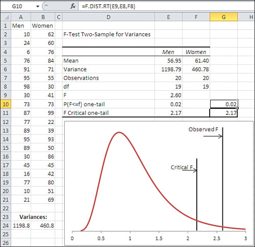
No one tells you—not the documentation, not the dialog box, not other books that deal with the Data Analysis add-in—that the data you designate as Variable 1 in the F-Test tool’s dialog box is always treated as the numerator in the F ratio.

The F-Test Tool Always Divides Variable 1 by Variable 2

Why is it important to know that? Suppose that your research hypothesis was that men have greater variability than women on whatever it is that you’ve measured in Figures 6.1 and 6.2. If you arranged things as shown in Figure 6.2, with the men’s measures in the numerator of the F ratio, then all is well. Your research hypothesis is that men have greater variability on this measure and the way you set up the F test conforms to that hypothesis. The test as you have set it up asks whether men’s variability is so much greater than women’s that you can rule out chance—that is, sampling error—as an explanation for the difference in their variances.

But now suppose that you didn’t know that the F-Test tool always places Variable 1 in the numerator and Variable 2 in the denominator. In that case, you might in all innocence instruct the F-Test tool to treat the women’s measures as Variable 1 and the men’s as Variable 2. With the data in Figures 6.1 and 6.2 you would get an F ratio of less than 1. You would be hypothesizing that men exhibit greater variability on the measure, and then proceeding to test the opposite.

As long as you knew what was going on, no great harm would come from that. It’s easy enough to interpret the results properly. But it could be confusing, particularly if you tried to interpret the meaning of the critical value reported by the F-Test tool. More on that in the following section.

The F-Test Tool Changes the Decision Rule

The F-Test tool changes the way the F ratio is calculated, depending on which data set is identified as Variable 1 and which as Variable 2. The tool also changes the way that it calculates the inferential statistics, according to whether the calculated F statistic is greater or less than 1.0. Notice the chart in Figure 6.2. The chart is not part of the output produced by the F-Test tool. I have created it using Excel’s F.DIST() worksheet function.

The curve in the chart represents all the possible F ratios you could calculate using samples of 20 observations each, assuming that both samples come from populations that have the same variance. (The shape of an F distribution depends on the number of observations in each sample).

At some point, the ratio of the sample variances gets so large that it becomes irrational to believe that the underlying populations have the same variance. If those populations have the same variance, you would have to believe that sampling error is responsible when you get an F ratio that doesn’t equal 1. It doesn’t take much sampling error to get an F ratio of, say, 1.05 or 1.10. But when you get a sample whose variance is twice that of the other sample—well, either an improbably large degree of sampling error is at work or the underlying populations have different variances.

“Improbably large” is a subjective notion. What is wildly unlikely to me might be somewhat out of the ordinary to you. So each researcher decides what constitutes the dividing line between the improbable and the unbelievable (often guided by the cost of making an incorrect decision). It’s conventional to express that dividing line in terms of probability. In the F-Test dialog box shown in Figure 6.1, if you accept the default value of .05 for Alpha, you are saying that you will regard it as unbelievable if something could occur only 5% of the time. In the case of the F-Test, you would be saying that you regard it as unbelievable to get a ratio so large that it could occur only 5% of the time when both populations have the same variance.

That’s what the vertical line labeled “Critical F” in Figure 6.2 is about. It shows where the largest 5% of the F ratios would begin. Any F ratio you obtained that was larger than the critical F value would belong to that 5% and, therefore, because you selected .05 as your Alpha criterion, would serve as evidence that the underlying populations had different variances.

The other vertical line, labeled “Observed F,” is the value of the actual F ratio calculated from the data in A2:B21. It’s the ratio of the variances, which are shown as the result of the VAR.S() function in A24:B24 and as returned by the F-Test tool as static, calculated values in E6:F6. The F-Test tool also returns the F ratio in E9, and it’s that value that appears in the chart as the vertical line labeled “Observed F.”

The observed F ratio of 2.60 in Figure 6.2 is even farther from a ratio of 1.0 than is the critical value of 2.17. So if you had used an alpha of .05, your decision rule would lead you to reject the hypothesis that the two populations that underlie the samples have equal variances.

But what happens if the investigator, not knowing what Excel will do about forming the F ratio, happens to identify the measures of women as Variable 1? Then the F-Test tool puts the variance for women, 460.8, in the numerator and the variance for men, 1198.8, in the denominator. The F ratio is now less than 1.0 and you get the output shown in Figure 6.3.

Figure 6.3. With the smaller variance now in the numerator of the F ratio, the results are still “significant” but reversed.

If you know what’s going on—and you do now—it’s not too hard to conclude that the observed F ratio of 0.38 is just as unlikely as 2.60. If the population variances are equal, the most likely results of dividing one sample variance by the other are close to 1.0. Looking at the two critical values in Figures 6.2 and 6.3, 2.17 at the high end and 0.46 at the low end cut off 5% of the area under the curve: 5% at each end. Whether you put the larger variance in the numerator by designating it as Variable 1, or in the denominator by designating it Variable 2, the ratio is unlikely to occur when the populations have equal variances, so if you accept 5% as a rational criterion you reject that hypothesis.

Understanding the F Distribution Functions

The cells G10:G11 in both Figures 6.2 and 6.3 contain worksheet functions that pertain to the F distribution. The F-Test tool does not supply them—I have done so—but notice that the values shown in G10:G11 are identical to those in E10:E11, which the F-Test tool does supply. However, the F-Test tool does not supply the formulas or functions it uses to calculate results: It supplies only the static results. Therefore, to more fully understand what’s being done by a tool such as the F-Test in the Data Analysis add-in, you need to know and understand the worksheet functions the tool uses.

Cell G10 in Figure 6.2 uses this formula:

=F.DIST.RT(E9,E8,F8)

The F.DIST.RT function returns a probability, which you can interpret as an area under the curve. The RT suffix on the function informs Excel that an area in the right tail of the curve is needed; if you use F.DIST() instead, Excel returns an area in the left tail of the curve.

The function’s first argument, which here is E9, is an F value. Used as an argument to the F.DIST.RT() function, the value in cell E9 calls for the area under the curve that lies to the right of that value. In Figure 6.2, the value in E9 is 2.60, so Excel returns 0.02: 2% of the area under this curve lies to the right of an F value of 2.60.

As noted in the prior section, the shape of an F distribution depends on the number of observations that form the variance in the numerator and in the denominator of the F ratio. More formally, you use the degrees of freedom instead of the actual number of observations: The degrees of freedom is the number of observations, minus 1. The second and third arguments to the F.DIST.RT() function are the degrees of freedom for the numerator and for the denominator, respectively.

You can conclude from the result returned by this function that, assuming men and women have the same variance in the populations, you would see an F ratio at least as large as 2.60 in only 2% of the samples you might take from the populations. You might regard it as more rational to conclude that the assumption of equal population variances is incorrect than to conclude that you obtained a fairly unlikely F ratio.

The formula in cell G11 of Figure 6.2 is as follows:

=F.INV(0.95,E8,F8)

Instead of returning an area under the curve, as F.DIST() and F.DIST().RT do, the F.INV() function accepts an area as an argument and returns an F value. Here, the second and third arguments in E8 and F8 are the same as in the F.DIST.RT() function: the degrees of freedom for the numerator and the denominator. The 0.95 argument tells Excel that the F value that corresponds to 95% of the area under the curve is needed. The function returns 2.17 in cell G11, so 95% of the curve lies to the left of the value 2.17 in an F distribution with 19 and 19 degrees of freedom. The F-Test tool returns the same value, as a value, in cell E11.

(The function’s INV suffix is short for inverse. The value of the statistic is conventionally regarded as the inverse of the area.)

Compare the functions in Figure 6.2 that were just discussed with the versions in Figure 6.3. There, this formula is in cell G10:

=F.DIST(E9,E8,F8,TRUE)

This time, the F.DIST() function is used instead of the F.DIST.RT() function. The F.DIST() function returns the area to the left of the F value that you supply (here, that value is 0.38, which is the value in cell E9, the ratio of the women’s variance to the men’s variance).

You can see by comparing the charts in Figures 6.2 and 6.3 that it’s as unlikely to get a ratio of 0.38 (women’s to men’s variance) as it is to get a ratio of 2.60 (men’s to women’s variance). But it can confuse the issue that the critical value is different in the two sets of output. It is 2.17 in Figure 6.2 because the F-Test tool is working with an F ratio that’s larger than 1.0, so the question is how much larger than 1.0 must the observed F ratio be in order to cut off the upper 5% of the distribution (or whatever alpha you choose instead of 0.05).

The critical value is 0.46 in Figure 6.3 because the F-Test tool is working with an F ratio that’s smaller than 1.0, so the question is how much smaller than 1.0 must the observed F ratio be in order that you consider it improbably small—smaller than the smallest 5% of the ratios you observe if the populations have the same variance?

That critical value of 0.46 in cell G11 of Figure 6.3 is returned by this formula:

=F.INV(0.05,E8,F8)

Whereas, as noted earlier, the formula in cell G11 of Figure 6.2 is this:

=F.INV(0.95,E8,F8)

In the latter version the function returns the F value that cuts off the lower 95% of the area under the curve: Thus, larger values have a 5% or smaller chance of occurring.

In the former version, the function returns the F value that cuts off the lower 5% of the area under the curve. This is the critical value you want if you’ve set up the observed F ratio so that the smaller variance is in the numerator.

There is an F.INV.RT() function that you might use instead of =F.INV(0.95,E8,F8). It’s simply a matter of personal preference. The F.INV.RT() function returns the F value that cuts off the right tail, not the left tail as the F.INV() function does. Therefore, these two functions are equivalent:

=F.INV(0.95,E8,F8)

and

=F.INV.RT(0.05,E8,F8)

Making a Nondirectional Hypothesis

So far we’ve been interpreting the F-Test tool’s results in terms of two mutually exclusive hypotheses:

• There is no difference between the two populations, as measured by their variances.

• The population of men has a larger variance than does the population of women.

The second hypothesis is called a directional hypothesis, because it specifies which of the two variances you expect to be the larger. (This is also called, somewhat carelessly, a one-tailed hypothesis, because you pay attention to only one tail of the distribution. It’s a slightly careless usage because, as you’ll see in later chapters, many nondirectional hypotheses make reference to one tail only in the F distribution.)

What if you didn’t want to take a position about which variance is greater? Then your two, mutually exclusive hypotheses might be the following:

• There is no difference between the two populations, as measured by their variances.

• There is a difference between the two populations, as measured by their variances.

Notice that the second hypothesis doesn’t specify which population variance is greater—simply that the two population variances are not equal. It’s a nondirectional hypothesis. That has major implications for the way you go about structuring and interpreting your F test (and your t-tests, as you’ll see in Chapter 9).

Looking at It Graphically

Figure 6.4 shows how the nondirectional situation differs from the directional situation shown in Figures 6.2 and 6.3.

Figure 6.4. In a nondirectional situation, the alpha area is split between the two tails.

In a case like the one shown in Figure 6.4, you do not take a position regarding which population has the larger variance, just that one of them does. So, if you decide that you’re willing to regard an outcome with a 5% likelihood as improbable enough to reject the null hypothesis, then that 5% probability must be shared by both tails of the distribution. The lower tail gets 2.5% and the upper tail gets 2.5%. (Of course, you could decide that 1%, not 5%, is necessary to reject an hypothesis, or any other value that your personal and professional judgment regards as “improbable.” The important point to note is that in a nondirectional situation, you divide that improbable alpha percentage between the two tails of the distribution.)

One of the consequences of adopting a nondirectional alternative hypothesis is that the critical values move farther into the tails. In Figure 6.4, the nondirectional hypothesis moves the upper critical value to about 2.5, whereas in Figure 6.2 the directional hypothesis placed the critical value at 2.17. (It is solely coincidence that the upper critical value is about 2.5 and cuts off 2.5% of the area.)

The reason the critical value moves is that in Figure 6.4, the critical values cut off the lower and upper 2.5% of the distributions, rather than the lower 5% or the upper 5%, as in Figures 6.2 and 6.3. Therefore, the critical values are farther from the center of the distribution in Figure 6.4.

Running the F-Test Tool for a Nondirectional Hypothesis

If you want to use a nondirectional hypothesis, halve the alpha level accordingly. Adjust the alpha level in the F-Test tool’s dialog box. If you want the overall alpha level to be 5%, enter 0.025 when you run the tool.

Specifying an alpha level affects only the critical F value returned by the F-Test tool. You can always look at the p-value for the observed F value returned by the tool (for example, cell E10 in Figure 6.3); then, decide whether the p-value is small enough to regard as improbable the hypothesis that the result is due to sampling error. In practice, it’s a matter of whether you want to think in terms of the probabilities (pay attention to alpha and the p-value) or in terms of the F values (think in terms of the observed and critical F ratios).

A Trap to Avoid

One thing you must not do if you have made a nondirectional hypothesis is to look at the data before deciding which group’s data to put in the F ratio’s numerator, by using that group as Variable 1 in the F-Test tool’s dialog box.

It’s legitimate to decide before seeing the data that you will treat whichever group has the larger variance as Variable 1. Not this: “I see that men have the greater variance, so I’ll treat their data as Variable 1.” But instead this: “I will put whichever group has the greater variance in the numerator of the F ratio by designating that group as Variable 1.”

It’s also legitimate to assign one of the two sets of data to Variable 1 with a coin flip or some other random event.

If you decide that you will always put the larger variance in the F ratio’s numerator, you will never get an F ratio that’s less than 1.0. You’re asking the upper tail of the distribution to stand in for the lower tail too. Therefore, if the test is nondirectional, you must be sure to put half the alpha that you really want in the dialog box. Notice that this is consistent with the advice I gave you in the prior section, to specify half the alpha you really want when you’re dealing with the F-Test tool’s dialog box, and you’re making a nondirectional alternative hypothesis.

The Available Choices

In summary, the way you set things up in the Data Analysis add-in’s F-Test tool depends on whether you make a directional or nondirectional hypothesis. The next two sections briefly discuss each alternative given that you set alpha, the probability that your observed result is due to chance, to 0.05.

Directional Hypotheses

Make the directional hypothesis that your theory leads you to support. If theory tells you that men should have a larger variance on some measure than women, let your alternative hypothesis be a directional one: that men have the larger variance. Use the F-Test tool’s dialog box to put the men’s variance in the numerator of the F ratio (set the men’s data as Variable 1) and set alpha to 0.05. Conclude that your alternative hypothesis is correct only if the observed F ratio exceeds the critical F ratio.

Do not reject the null hypothesis of no difference even if the men’s sample variance is significantly smaller than the women’s. Once you’ve made a directional hypothesis that points in a particular direction, you must live with it. It’s capitalizing on chance to make a directional hypothesis after you’ve seen what the outcome is.

Nondirectional Hypotheses

Make a nondirectional hypothesis that the sampled populations have different variances, but don’t specify which is greater. For convenience, treat the group with the larger variance as Variable 1, cut the alpha in half when you complete the dialog box entries, and run the F-Test tool once. If the reported p-value is less than half the nominal alpha, adopt your alternative hypothesis that the populations have different variances.

A Final Point

Ignore the F-Test’s output label “P(F<=f) one-tail.” The label itself is misleading, the symbols are undefined, and it remains the same whether the obtained F ratio is larger or smaller than the critical value. Furthermore, the probability that one value is less than or equal to another is either 1.0 or 0.0: Either it is or it isn’t. The values “F” and “f” are two specific numbers, and a statement such as “The probability that 2.60 is greater than 2.17 is .02” has no meaning.

To the contrary: in the F-Test tool’s output, the quantity labeled “P(F<=f) one-tail” is the probability of obtaining the observed F ratio under the assumption that the populations from which the samples were taken have the same variance.