
Chapter 15
Parallel Track Fitting in the CERN Collider
What's in This Chapter?
Introducing particle track fitting
Introducing Intel Array Building Blocks
Parallelizing programs using Intel Array Building Blocks
This chapter looks at parallelizing code that determines particle tracks within high-energy physics experiments. This represents some of the work done at the CERN GSI establishment in Darmstadt, Germany. The group is well known for its discovery of the elements bohrium, hassium, meitnerium, darmstadtium, roentgenium, and copernicium.
Intel Array Building Blocks (ArBB) is a research project, and consists of a C++ template library that provides a high-level data parallel programming solution. By using ArBB to parallelize software, you can produce thread-safe, future-proofed applications. The six hands-on activities let you try out parallelizing a serial track-fitting program using ArBB.
The Case Study
The Compressed Baryonic Matter (CBM) project is designed to explore the properties of super-dense nuclear matter by using a particle accelerator to collide charged particles against a fixed target.
The word baryonic in the project title refers to baryons, large particles made up of three quarks — a quark being an elementary particle from which all matter is made. Quarks are found neither on their own nor in isolation.
One of the aims of the CBM experiment is to search for the transition of baryons to quarks and gluons (the particles that hold together the quarks). The CBM project is carried out at GSI (center for heavy ion research) and its adjacent facility FAIR (Facility for Antiproton and Ion Research) in Darmstadt, Germany. Researchers from around the world use this facility for experiments using the unique, large-scale accelerator for heavy ions. You can find more information about CBM at www.gsi.de/forschung/fair_experiments/CBM/index_e.html.
The Stages of a High-Energy Physics Experiment
Generally, a high-energy physics experiment goes through eight stages, as shown in Figure 15.1.
Figure 15.1 The stages of a high-energy physics experiment
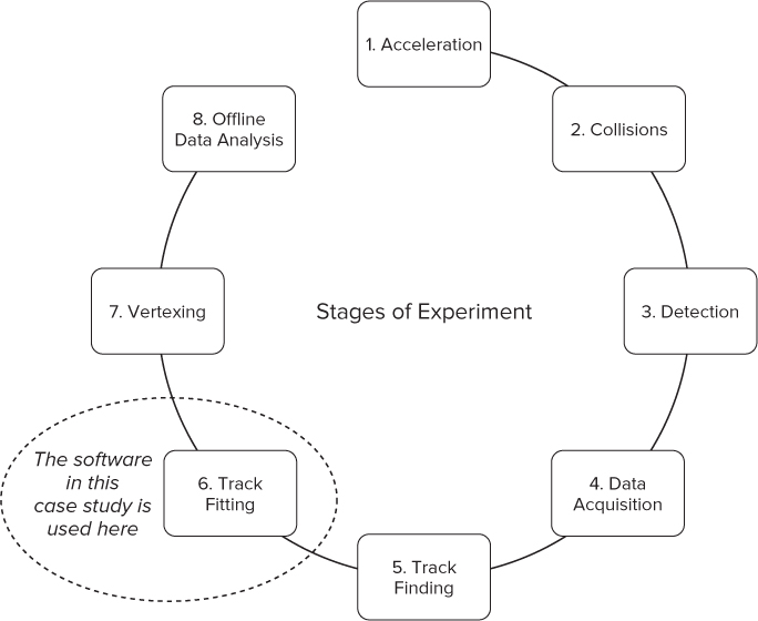
- In the first two steps, acceleration and collision, particles are accelerated to almost the speed of light and then collided against a fixed target or against other accelerated particles.
- In the next two steps, detection and data acquisition, particles are detected as they pass through detector planes. In the case of the CBM experiment, there are seven such planes, referred to as stations. Each station records the position of particles passing through them — these are the particle hits. The collected data is then used to determine what actually happened.
- The track-finding and the track-fitting stages are used to reconstruct the path that the particles took. Track finding determines which hits in the various stations belong to which track. Track fitting is used to take into account the inaccuracies of the detection system. The station data and its extraction are noisy, resulting in inaccurate hit coordinates. An attempt is made to eliminate these inaccuracies and refine the particle tracks. The method involves the use of a Kalman filter and is the subject of this case study.
- At the vertexing stage, various constraints to the tracks are applied. For example, a particular particle may decay along its track and produce a number of other tracks, all of which must originate from the same point. This is an attempt to find correlation between tracks.
- Finally, the captured data is used for offline data analysis and the physical interpretation of events.
The Track Reconstruction Stages
The CBM experiment looks at hadrons, electrons, and photons emitted in heavy-ion collisions. Once each particle is detected, the correct path or track has to be calculated, the data then being used to help interpret what has happened.
Each event (collision) results in many thousands of potential tracks passing through the detectors. These events can be repeated many thousands of times per second, requiring extremely high data-processing rates. Modern high-energy physics experiments typically have to process terabytes of input data per second. The track-reconstruction stages are the most time-consuming parts of the analysis; therefore, the speed of any track-determination algorithms becomes very important in the total processing time.
Track determination would be trivial were it not for complications arising because of inaccuracies due to detector noise and scattering due to electric charge, energy loss, nonuniform magnetic fields, and so on.
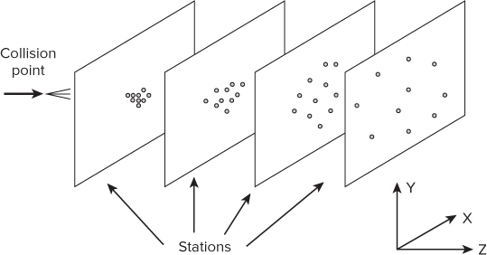
Figure 15.2 shows a typical problem, with multiple planes positioned at different z positions across the trajectories of the particles. Each plane registers the x and y positions of the particles as they pass through (referred to as hits). The problem then becomes to reconstruct the paths of the various particles by using their positions on each detector.
Figure 15.2 Typical hits at stations along trajectory
Listing 15.1 shows the structure used to store the station information. The code is much reduced; if you want to see the original code, look in the class.h file from the hands-on project (see Activity 15-1). Notice that the class contains 15 different pointers (for example, *z). Each pointer gets allocated dynamic memory within the init method, which is called by the Stations constructor.
Notice, too, that when malloc is used in the init() function, it creates enough space for all the stations. This is true for all 15 pointers that you can see.
 Listing 15.1: The Stations class in the serial version of the code
// NOTE: See class.h for complete listing.
// The listing here is not intended to be compiled.

class Stations{
public:
  int nStations;

  ftype *z, *thick, *zhit, *RL, *RadThick,*logRadThick,*Sigma,*Sigma2,*Sy;
  ftype (**mapX), (**mapY), (**mapZ); // polinom coeff.

  void initMap( int i, ftype *x, ftype *y, ftype *z){// init code }
  Stations( int ns )    {init( ns );}
  void init( int ns )
  {
    // allocate memory all 7 stations are together
    nStations = ns;
    z = (ftype*)malloc(ns*sizeof(ftype));
    // … repeat for thick zhit RL RadThick logRadThick Sigma
    // Sigma2 Sy mapX mapY mapZ mapXPool mapYPool mapZPool
  }

  ∼Stations()    {// free dynamically allocated memory}

private:
  // pointers to private pool
  ftype *mapXPool, *mapYPool, *mapZPool;
};
code snippet Chapter1515-1.h
Track Finding
Track finding involves determining which hits on each of the planes were made by the same particle, therefore indicating its path through the detector. This is time-consuming and involves using the properties of a particle (spatial, velocity, mass, charge) at one plane to predict its hit position on the next plane. Once the prediction has been made, a search is made for the closest hit.
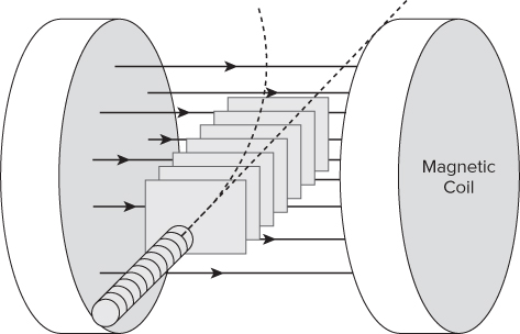
To make matters more interesting, the whole detector is embedded within a magnetic field, so any charged particles will respond accordingly (see Figure 15.3). The direction and radius of any trajectory curvature depend on the strength and polarity of the charged particle.
Figure 15.3 Detector stations embedded within a magnetic field
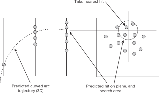
A lot of track finding can be related to pattern recognition, which is something humans are particularly good at, and which computers are not. Figure 15.4 shows a predicted hit on the last plane after using the two previous hits to fit a predicted curved arc. The nearest measured hit is then taken.
Figure 15.4 Using prediction to determine the next hit
Listing 15.2 shows the Tracks class that is used to hold all the track information. At run time more than 20,000 track details are held in the instantiation of this class. Notice, again, like the Stations class previously discussed, a number of pointers are used to hold dynamically allocated memory. When ArBB is added to the code, one of the first things to address is to replace the dynamically allocated structures with ArBB containers.
Listing 15.2: The Tracks class in the serial version of the code
// NOTE: See class.h for complete listing.
// The listing here is not intended to be compiled.

class Tracks
{
public:
  unsigned int nStations;
  unsigned int nTracks;

  ftype *MC_x, *MC_y, *MC_z, *MC_px, *MC_py, *MC_pz, *MC_q;
  int *nHits, *NDF;
  ftype **hitsX, **hitsY;
  ftype *hitsX2, *hitsY2;
  int **hitsIsta;

  void init( int ns, int nt )
  {
    nTracks = nt;
    MC_x = ( ftype* ) malloc( sizeof( ftype ) * nt );

    // repeat for : MC_y MC_z MC_px MC_py MC_pz MC_q  nHits
    // NDF hitsX  hitsY  hitsIsta

    memXPool = ( ftype* ) malloc( sizeof( ftype ) * nt * nStations );
    // repeat for : memYPool  memIstaPool hitsX2 hitsY2
  }

  ∼Tracks()    {}

  void setHits( int i, int *iSta, ftype *hx, ftype *hy )
  {
    // record hits
  }

private:
  ftype *memXPool, *memYPool;
  int *memIstaPool;
};
code snippet Chapter1515-2.h
Track Fitting
After determining the track by successive plane hits, track-fitting algorithms are then applied to smooth out any track irregularities due to inaccuracies along the paths. This forms the bulk of the work in this case study.
Successive station hits of a particular track may not follow a highly accurately determined track, due to noise and other inaccuracies. Track fitting is used to minimize how close the measured hits are to what they are assumed to be for a particular fit hypothesis. By using a particle's location at one station, the environment between it and the next station, together with the physical properties of the particle, a prediction can be made as to where the particle will hit the following station. A weighted average is then taken between the recorded hit position and the predicted hit position to determine the actual particle position.
Kalman Filter Overview
The Kalman filter is a mathematical method designed to filter out noise and other inaccuracies in measurements observed over time. It is used in almost all high-energy physics experiments to carry out track fitting. The Kalman filter calculates estimates of the true values of measurements recursively over time using incoming measurements and a mathematical process model.
Determining a track requires two things:
- A model that approximates the track's trajectory
- An understanding of the physical properties of the detector
The Kalman filter is very good at this because it can determine the presumed path and take all the complications of an irregular topology (both of the physical detector and nonlinear magnetic field) in its stride.
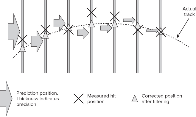
Figure 15.5 shows a Kalman filter-based track fitting. As more track hits are corrected, the confidence about the track is increased and the predicted precision becomes higher. This is shown in the illustration by the decreasing thicknesses of the prediction arrows. Various filtering effects are applied to arrive at the final track's trajectory positions.
Figure 15.5 Using a Kalman filter to obtain an accurate path
Kalman Filter Steps
Figure 15.6 shows the steps of a Kalman filter. The symbol r is the state vector of the particle at each plane (position and velocity), and C is the covariance (confidence) matrix. The other symbols represent the magnetic field and various states of the system:
Figure 15.6 The Kalman filter operation
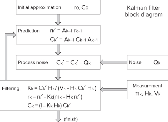
- The initial approximation step sets an approximate value of the vector r0 and the covariance matrix C0.
- The prediction step describes the deterministic changes of the vector over time to an adjacent station.
- The process noise step describes probabilistic deviations of the vector due to noise (Qk), and so on.
- The final step filters the actual values Mk, Hk, and Vk, taking into account the previous three steps.
The CBM team at GSI has implemented a fast Kalman filter for use in the track-fitting stage of their high-energy particle analysis. For each track, two arrays are maintained — one for particle state (position, velocity, and momentum), and another for the covariance values used for determining trajectory confidence. The filter is applied to each track in turn at each station along its trajectory to smooth out inaccuracies and errors, and used to derive a corrected track position.
The filter has been implemented using single-precision floating-point calculations. (Traditional Kalman filters use double precision.) Additional research has been applied to ensure that working with single precision gives an accurate enough result. Using single precision over double reduces the space needed to store the data by half and results in faster calculations.
What Is Array Building Blocks?
ArBB is C++ template library that provides a high-level data parallel programming solution intended to free developers from dependencies on low-level parallelism mechanisms and hardware architectures.
ArBB is designed to take advantage of multi-core processors, many-core processors, and GPUs. Under normal use, ArBB applications are automatically free of data races and deadlocks. Its main features are as follows:
- Has its own embedded language
- Uses dynamic compilation with just-in-time (JIT) compiler
- Provides implicit parallelism for computationally intensive maths
- Works across multiple cores and varying SIMD widths
- Provides structured data parallelism (patterns) with no data races
- Uses separate memory space with no pointers
- Does not require synchronization primitives
The essence of ArBB is collections (containers) and their associated operators. Collections are designed to work on arrays. The arrays can be any size and dimension, regularly or irregularly shaped. Containers either are bound to existing C/C++ data and take on the size and shape of the bound data, or they can be constructed independently without any binding. An ArBB range is used to transfer data from the ArBB code to the C/C++ code.
Once a set of containers is bound to existing data entities, you can work on them as though they were single variables. For example, if containers A, B, and C have been declared and bound to three separate C/C++ arrays (of any dimension), they may be processed as if normal single variables:
![]()
ArBB will produce executable code that fully utilizes any SIMD instructions and multiple cores available to carry out the operation. This is done without any further intervention by the programmer.
In general, when a container appears on both the left and right side of an expression, ArBB generates a result as if all the inputs were read before any outputs are written. In practice, you must put this expression within a function and invoke that function with a call operation.
ArBB is delivered as a library that provides data collections, operators for data processing, and an associated syntax.
As shown in Figure 15.7, the application code is written in C/C++ and looks like fairly standard nonthreaded code. You add ArBB code using a C++ API.
Figure 15.7 The ArBB platform
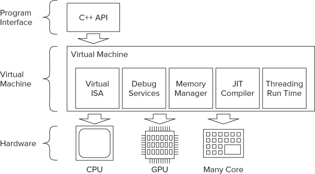
The ArBB runtime uses a virtual machine (VM) and employs a just-in-time (JIT) compiler. The VM works out at run time the best performance paths based on its knowledge of the hardware platform. By deferring the final compilation of the ArBB code until it resides on the target platform, the JIT compiler can produce architecture-specific optimized code.
Listing 15.3 is a program that shows a simple ArBB program. The sum_of_differences function will be compiled and executed at run time; the main function is a normal C++ function and is compiled in the usual way.
The main function has two dense containers, a and b, similar to the STL's std::vector, whose size is set to 1024.
The first time you run the application, the ArBB call operator causes the JIT compiler to compile sum_of_differences. The ArBB code is then executed. If there were further calls to the function sum_of_differences, it would not need to be recompiled.
Listing 15.3: An ArBB program skeleton
#include <arbb.hpp>
#include <cstdlib>

void sum_of_differences(dense<f32> a, dense<f32> b, f64& result)
{
  result = add_reduce((a – b) * (a - b));
}

int main()
{
  std::size_t size = 1024;
  dense<f32> a(size), b(size);
  f64 result;
  range<f32> data_a = a.read_write_range();
  range<f32> data_b = a.read_write_range();

  for (std::size_t i = 0; i != size; ++i) {
    data_a[i] = static_cast<float>(i);
    data_b[i] = static_cast<float>(i + 1);
    call(&sum_of_differences)(a, b, result);
    std::cout << "Result: " << value(result) << ‘
’;
  }
  return 0;
}
code snippet Chapter1515-3.cpp
The big advantage of ArBB is the optimization performed by the JIT compiler. Because the ArBB code is compiled at run time, you can optimize the code to take advantage of the hardware it is running on. When you introduce the same code to a newer-generation CPU, the code will be optimized to match the new features available in the CPU.
Parallelizing the Track-Fitting Code
In the case study, a serial version of a track-fitting benchmark was parallelized using ArBB.
Adding Array Building Blocks to Existing Code
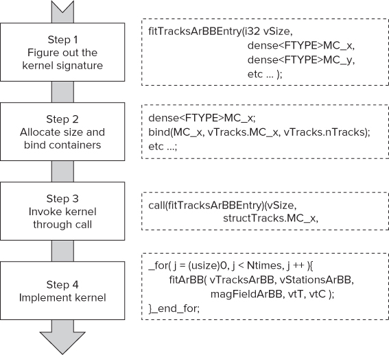
Figure 15.8 shows the steps to convert a serial program into a parallel ArBB program:
Figure 15.8 Converting a serial program to a parallel ArBB program
In the “Hands-On Project” section later in this chapter, you apply these steps to the filter driver code.
Code Refactoring
Some of the original code required more reworking before the preceding four steps were carried out:
- Any references to global variables were removed so that access was by parameters passed in via the function call.
- A wrapper function was inserted in the call stack to help marshal the parameters and data structures.
- The code that was to be made parallel was changed to an inline function. This was done so that it would be easy to change the size of the data types within the code.
- Some local variables were moved into a higher-level function with the address being passed in.
- Each array of structures (AoS) was changed to a structure of arrays (SoA).
An Example of Class Change
Listing 15.4 shows a cut-down version of the StationsArBB class. This is the ArBB replacement for the Stations class shown in Listing 15.1. Note that all the variables are now dense containers and that there is no dynamic memory allocation.
Listing 15.4: The ArBB version of the Stations class
/! define stations (SOA)
// NOTE: See arbb_classes.h for complete listing.
// The listing here is not intended to be compiled.

template<typename U>
class StationsArBB
{
public:
  dense<U> z, thick, zhit, RL, RadThick, logRadThick, Sigma, Sigma2, Sy;
  dense<U, 2> mapX, mapY, mapZ; // polynomial coeff.
public:
  StationsArBB(){};
  void field( const usize &i, const dense<U> &x,
  const dense<U> &y,   dense<U> H[3] )
  {
    dense<U> x2 = x*x;
    // etc  …
  }
};
code snippet Chapter1515-4.h
An Example of Kernel Code Change
Listing 15.5 shows the changes that were done to the main loop in the Kalman filter. You can see how the structure of the ArBB code is similar to the original serial code:
- The C for loop is replaced by an ArBB _for loop.
- The order and names of functions called are the same.
- Some new ArBB types are used in place of the C types.
If you want to compare the changes for yourself, you can find the original source code for the Kalman filter in the file serial_KF.cpp, with the converted code being in parallel_KF.cpp.
Listing 15.5: Example of loop in Kalman filter (ArBB and serial code)
// NOTE THIS CODE IS INCOMPLETE AND WILL NOT COMPILE!
// IT IS INCLUDED HERE FOR COMPARISON PURPOSES ONLY

SERIAL VERSION

for( --i; i>=0; i-- ){
  //   h = &t.vHits[i];
  z0 = vStations.z[i];
  dz = (z1-z0);
  vStations.field(i,T[0]-T[2]*dz,T[1]-T[3]*dz,H0);
  vStations.field(i,vTracks.hitsX[iTrack][i],vTracks.hitsY[iTrack][i], HH);
  combine( HH, h_w, H0 );
  f.set( H0, z0, H1, z1, H2, z2);

  extrapolateALight( T, C, vStations.zhit[i], qp0, f );

  addMaterial( iTrack, i, qp0, T, C );
  filter( iTrack, xInfo, vTracks.hitsX[iTrack][i], h_w, T, C );
  filter( iTrack, yInfo, vTracks.hitsY[iTrack][i], h_w, T, C );
  memcpy( H2, H1, sizeof(ftype) * 3 );
  memcpy( H1, H0, sizeof(ftype) * 3 );
  z2 = z1;
  z1 = z0;
}

ARBB VERSION

// Note ‘U’ is a template parameter and becomes an ArBB floating point type
_for( i -= 1, i >= 0, i-- ){
  U z0 = ss.z[i];
  dz = z1 - z0;
  ss.field( i, T[0] - T[2] * dz, T[1] - T[3] * dz, H0 );
  ss.field( i, ts.hitsX2.row( i ), ts.hitsY2.row( i ), HH );
  combineArBB<U>( HH, w, H0 );

  //! note: FieldRegionArBB f sets values here, needn't pass parameters
  f.set( H0, z0, H1, z1, H2, z2);

  extrapolateALightArBB2<U>( T, C, ss.zhit[i], qp0, f );
  addMaterialArBB( ts, ss, i, qp0, T, C );
  filterArBB( ts, ss, xInfo, ts.hitsX2.row( i ), w, T, C );
  filterArBB( ts, ss, yInfo, ts.hitsY2.row( i ), w, T, C );
  for( int j = 0; j < 3; j ++ ){
    H2[j] = H1[j];
    H1[j] = H0[j];
  }
  z2 = z1;
  z1 = z0;
}_end_for;
code snippet Chapter1515-5.h
Changing to Structure of Arrays
One of the changes made in the project was how data structures are used. In the original project there were a number of places where a data structure was held as an array of structures (AoS); these were changed to structures of arrays (SoA). Actually, ArBB automatically transforms each AoS to an SoA, but relying on the automatic transformation has some associated penalties:
- Host pointers cannot be aliased in a relaxed safety model.
- De-interleaving/interleaving needs to happen (“copy-in,” “copy-out”) explicitly/implicitly.
- Explicit control for transfer and control of memory “mirror space” is often a must.
Figure 15.9 shows that by using an SoA rather than an AoS, the layout in memory of the data elements is contiguous. The user-defined type whatever_udt has two member items, m_index and m_value. If the ArBB dense container is declared using the class whatever_udt, it looks like an AoS — the dense container data being equivalent to an array, and the class whatever_udt being the structure. If you look at the layout in memory, you will see that to access a series of, say, three m_index values, the address locations are not next to each other.
Figure 15.9 Using SoA helps to keep memory access contiguous
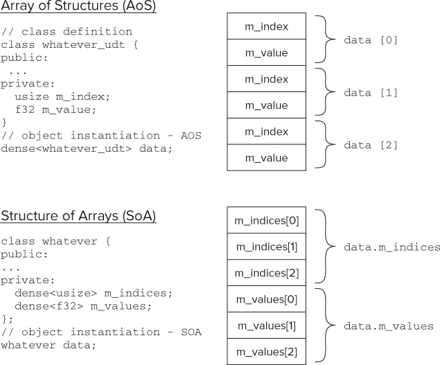
To get optimal performance, it is much better to restructure the class to be like a structure of arrays.
In object-oriented programming, some programmers will naturally write their code like the first example (SoA), but the better way from a performance point of view would be to write code like the second example (AoS). The first example is not incorrect; it just carries a higher overhead.
The Results
For the results of the parallel version of the track-fitting software to be of any use, the program must produce correct results and produce them fast. Let's consider the following aspects:
- Correctness
- Speedup and scalability
- Parallelism and concurrency
Correctness
A special version of the track-fitting software was written that compared the serial and parallel versions. This version first runs the serial code, obtaining the minimum time over five attempts, as before. Then the parallel version is run, again obtaining the minimum time over five attempts. The results of the parallel run are compared against the serial run to make sure that no errors exist.
Figure 15.10 shows the results of running the special version, showing no errors and a speedup factor of more than 43. The machine used has a two-socket motherboard containing two Intel Xeon X5680 (3.33GHz) processors, 12 GB of memory running Microsoft Windows 7 (64-bit). Each CPU has 6 cores and supports hyper-threading, giving a total availability of 24 hardware threads. Remember, your timings may differ.
Figure 15.10 The results show a huge speedup with no errors
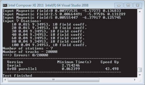
Figure 15.11 shows graphs of the residuals and pulls. Residuals show the deviation between simulated and estimated values. Pulls are a measure of the correctness of the error propagation. The reco and mc labels in the graphs refer to reconstructed values and true Monte-Carlo values, respectively.
Figure 15.11 The parallel results showing residuals and pulls of the estimated track parameters

These results are identical to the serial version (not shown), proving that the ArBB version and the original version have the same track quality.
Speedup and Scalability
Figure 15.12 shows how well the parallel program responds to different numbers of hardware threads. As you can see, there is a respectable speedup factor of almost 11 when using all 24 hardware threads available. The baseline for the speedup is the time the program takes when running one thread (not to be confused with the serial version). The speedup is calculated as follows:
![]()
Figure 15.12 The scalability and efficiency of the ArBB version
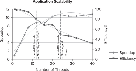
Using the lower number of threads, the parallel program runs at its most efficient; as the number of threads increases, the efficiency deteriorates. The two dotted lines in the graph mark the point where the number of ArBB threads is equal to the number of physical and logical cores (that is, hardware threads), respectively. Each of the 12 physical cores supports hyper-threading, giving a total of 24 logical cores.
Once the number of ArBB threads exceeds the number of hardware threads that the test machine can support, the speedup begins to drop — this is most likely due to the extra context switching the operating system has to perform.
The efficiency figure in Figure 15.12 is a measure of how well the CPU resources are being used. If a program uses all the CPU cycles available, it is said to be 100 percent efficient. The efficiency is calculated as follows:
![]()
The number of cycles used was measured using Amplifier XE's Lightweight Hotspots analysis. To measure the scalability and efficiency of the program, two program modifications are made:
- Amplifier XE's Frame API is used to insert markers at the beginning and end of the measurement points in the code:
#include "ittnotify.h"  // to use Amplifier XE API
_itt_domain* pD = _itt_domain_create( "TrackFitter" );
pD->flags = 1; // enable domain
for(i=0; i<NUM_RUNS;i++)
{
  // create time variable
  double time;
  {
    // start ArBB scoped timer which will measure
    // time within its scoped lifetime
    // start a frame for vtune
    _itt_frame_begin_v3(pD, NULL);
    const arbb::scoped_timer timer(time);
    // call main parallel track-fitting function
    fitTracksArBB( T1, C1, nT, nS );
  }
  // scoped time ends here, var time holds its value
  // reset Timing to minimum time so far
  Timing = std::min(Timing, time);
  _itt_frame_end_v3(pD, NULL);
}
- The ArBB API is used to control the maximum number of ArBB threads the ArBB kernel can use:
#include "arbb.hpp"    // to access the ArBB libraries
. . .
int main(int argc, char* argv[])
{
  …
  int num_threads = 0;
  if(argc==2)
  {
    num_threads=atoi(argv[1]);
    arbb::num_threads(num_threads);
    printf("WARNING: Max threads set to: %d
",num_threads);
  }
…
}
Parallelism and Concurrency
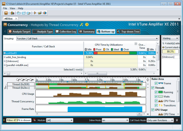
Figure 15.13 shows the screenshot of an Amplifier XE Concurrency analysis. The timeline view at the bottom half of the screen displays two of the threads, a CPU Usage line, a Thread Concurrency line, and a Frame Rate line.
Figure 15.13 The ArBB version of the application is highly parallel
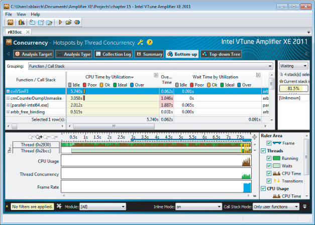
Notice the following:
- For most of the program, only one thread appears to be running. This is because the early part of the program was taken up with reading the data files and doing the JIT compilation.
- There is a blip of activity at the end of the program. Both the Thread Concurrency bar and the CPU Usage bar show that there is significant parallel activity. This is when the main track fitting is done.
Zooming in on a dense area of activity gives a better view of what is happening (see Figure 15.14). The timeline shows five distinct periods of activity — hence, the bumps in the CPU Usage bar.
Figure 15.14 The CPU Usage bar confirms that all 24 hardware threads are being used
At the beginning of each area period of activity is a vertical bar. This bar is a thread transition/synchronization point. When you hover your mouse over one of the transition lines, the gray box pops up and displays information about the synchronization object. It is a critical section in the Threading Building Blocks (TBB) scheduler. ArBB relies on its implementation of parallelism by using TBB under the hood.
In the top half of the screenshot is a bar that indicates how parallel this part of the program is — that is, the concurrency:
- The first tenth of the bar is colored red. (Sorry, you won't see the color in the printed version of the figure.) This means for 10 percent of the time the concurrency was poor.
- The next seven-tenths of the bar is colored orange, meaning that for 70 percent of the time the amount of parallelism is okay.
- The last two-tenths of the bar is colored green, meaning that for 20 percent of the time the concurrency level was perfect, with the number of the threads running being equal to the number of hardware threads the system can support.
The Hands-On Project
This section leads you through the steps to change the serial version of the track-fitting code to use ArBB. Two modules, the driver driver.cpp and the filter serial_KF.cpp, will be converted to using ArBB. This example takes one significant shortcut: the ArBB version of the filter is provided “ready-made.” You still have the opportunity of going through the four steps to add ArBB, because the filter driver code has to be “ArBB-ized.”
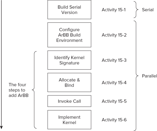
The Activities
Figure 15.15 shows the steps to perform. You start with a serial version of the code and progressively convert the program to use ArBB. The most significant parts of the hands-on are in Activity 15-3 to Activity 15-6. The steps you take here are typical of the steps you can take when adding ArBB to any project.
Figure 15.15 The steps of the hands-on activities
The Projects
The following three projects are provided with this case study:
- serial_track_fit — Contains the serial version of the track-fitting software. This is the version you will copy and modify.
- ArBB_track_fit — This is the solution. Your version should look like this once you have completed the hands-on activities.
- combined_track_fit — This version runs both the serial and parallel versions and checks their accuracy against each other and compares their run times. This version is not used in the hands-on, but it is supplied in case you are interested in looking how to validate the results. (Figure 15.10 showed an example of the output.)
Building and Running the Serial Version
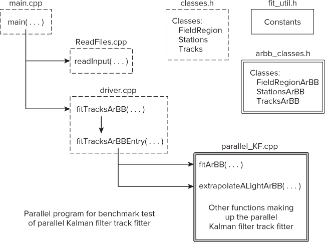
Figure 15.16 shows the files included in the serial version of the track-fitting software:
Figure 15.16 Configuration of the serial benchmark program
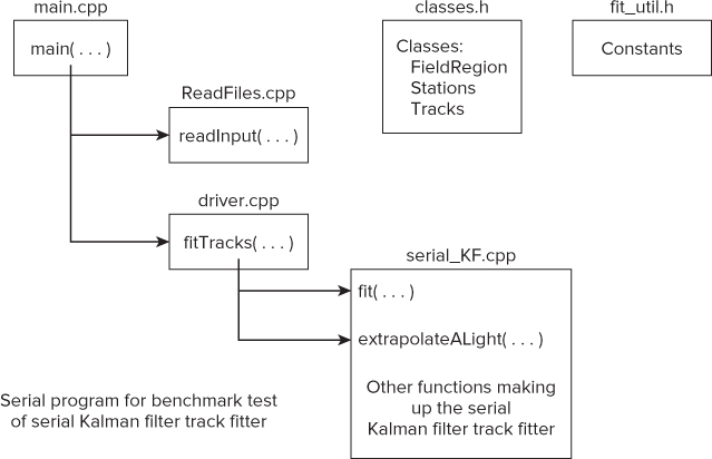
- main.cpp — Contains the main function of the program.
- ReadFiles.cpp — Contains the function readInput, which reads two data files, Geo.dat and Tracks.dat. This function creates dynamic arrays into which it places the information. The addresses of these arrays are stored within the pointer data of the three classes defined within the header file classes.h.
- driver.cpp — Contains the driving function fitTracks of the serial Kalman filter.
- serial_KF.cpp — Contains the serial version of the Kalman filter.
- classes.h — Contains three classes, for magnetic fields, stations, and tracks. Their data consists of pointers that are loaded with the start addresses of the dynamically allocated arrays created and loaded within ReadFiles.cpp.
- fit_util.h — Contains a set of constant values.
The Serial Track-Fitting Code
The track-fitting code first applies the Kalman filter to all 20,000 tracks and then repeats this 100 times, obtaining a time for doing so. This is then repeated five times, with the smallest of the five results taken as the final benchmark time.
Following is the main loop at the heart of the main function in main.cpp that calls the Kalman filter driver fitTracks five times. The time taken for each iteration is measured and stored in the Elapsed variable. The iteration that records the smallest time value is accepted as the benchmark timing. On Windows, the serial version uses timeGetTime() to record the timestamps.
for(i=0; i<NUM_RUNS;i++)
{
  // set start time
  StartTime = timeGetTime();
  // call main serial track-fitting function
  fitTracks( T1, C1, nT, nS );
  // determine elapsed time
  Elapsed = (int)(timeGetTime() - StartTime);
  // get minimum time so far
  Timing = std::min(Timing, Elapsed);
}
The T1 parameter is a pointer to an array that holds the track information; the C1 parameter points to the covariance matrix; and the nT and nS parameters are used to store the number of tracks and stations, respectively.
Listing 15.6 shows the driver.cpp file, which contains the driver function fitTracks, which is called from main(). The Kalman filter track fitter fit( i, T[i], C[i] ) is applied to each track in turn. This is then repeated 100 times to get an overall average performance. Once this has been carried out, the state and covariance data matrices for each track are extrapolated back to their start. In this hands-on, the most significant code edits will be made in driver.cpp.
Listing 15.6: The serial version of driver.cpp
#include <math.h>
#include "fit_util.h"         // set of constants
#include "classes.h"          // Main Kalman filter classes

typedef float ftype;          // set ftype to be single precision data

using namespace std;

extern FieldRegion  magField;
extern Stations     vStations;
extern Tracks       vTracks;

// -------------------------- Prototypes
void fit( int iTrack, ftype T[6], ftype C[15] );
void extrapolateALight( ftype T[], ftype C[], const ftype zOut, ftype qp0,
                                 FieldRegion &F );

// ***** Driver of Serial Version of Kalman Filter Track Fitter *****
void fitTracks( ftype (*T)[6], ftype (*C)[15], int nT, int nS )
{
  // Repeat the Kalman filtering 100 times
  for( int times=0; times<Ntimes; times++)
  {
    // take each track in turn and process
    for( unsigned int i=0; i<nT; i++ )
    {
      // apply Kalman filter to track
      fit( i, T[i], C[i], nT, nS );
    }
  }
  // extrapolate all tracks back to start
  for( unsigned int i=0; i<nT; i++ )
  {
    extrapolateALight( T[i], C[i], vTracks.MC_z[i], T[i][4], magField );
  }
}
code snippet Chapter1515-6.cpp
The Application Output
Figure 15.17 shows the output from the program. After displaying some setup information involving magnetic fields and the number of stations and tracks, the timing information is given. In this example, the time shown is just under three seconds. You need to be patient, however, because this is the best of five attempts; the actual run time is in excess of 15 seconds. You can build and run the serial version of the program for yourself in Activity 15-1.
Figure 15.17 Results of running the serial version of track-fitting software
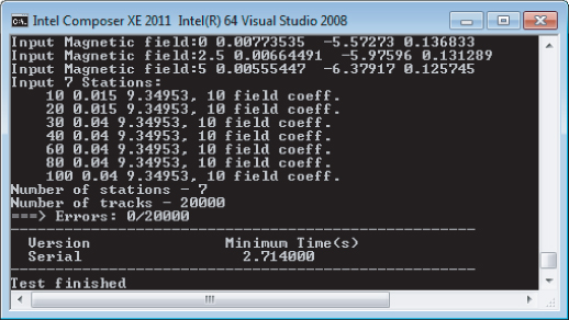
The machine used has a two-socket motherboard containing two Intel Xeon X5680 (3.33GHz) processors, 12 GB of memory running Microsoft Window 7 (64-bit). Each CPU has 6 cores, and supports hyper-threading, giving a total availability of 24 hardware threads. Remember, your timings may vary.
Building the Program
nmake -f Makefile-WIN32 clean
nmake -f Makefile-WIN32
Running the Program
serial-intel64.exe
Other Activities
CPP=cl
Parallelizing the Track-Fitting Code
As stated earlier, the Kalman filter is already provided for you with the complete ArBB code; however, you still need to modify the driver code.
Configuring the Array Building Blocks Build Environment
Some files will need to be modified, and others replaced. (You can try this for yourself in Activity 15-2.)
- The main function should call the new parallel driver fitTracksArBB.
- The ArBB-aligned functions for dynamic memory allocation and deallocation are added to the files classes.h and ReadFiles.cpp.
int lNHits = 100;
int *lIsta = (int*)arbb::aligned_malloc(lNHits*sizeof(int));
// some code to use
// etc …
// now free the dynamic structure
arbb::aligned_free( lIsta );
- The new parallel Kalman filter parallel_KF replaces the serial version serial_KF.cpp.
The new filter is provided already built. It was developed using the same methodology as the driver — that is, identify the kernel, bind and allocate, add the call, and implement the kernel.
Figure 15.18 shows the new configuration for the parallel version. New files have a double line around them; original files that need editing have a dotted box around them; original unmodified files have a single box around them.
Copying Files and Modifying the Makefile
- Add the following lines to the top of the file, making sure that the path ARBB_ROOT points to the place where you installed ArBB:
ARBB_ROOT = c:PROGRA∼2IntelarbbBeta5∼1
ARBB_INCS="$(ARBB_ROOT)include"
ARBB_LIBS="$(ARBB_ROOT)lib$(TARGET_ARCH)"
- Change the following lines:
EXE=serial-$(TARGET_ARCH).exe
serial_build: driver.obj main.obj ReadFiles.obj serial_KF.obj
  $(CPP) /o $(EXE) $** winmm.lib
EXE=parallel-$(TARGET_ARCH).exe
build: driver.obj main.obj ReadFiles.obj parallel_KF.obj
  $(CPP) /o $(EXE) $** /link /LIBPATH:$(ARBB_LIBS) arbb.lib
- Save your changes.
Modifying main.cpp
- Add an extra include:
#include <limits>         // for data limits
#include "arbb.hpp"       // to access the ArBB libraries
#include "fit_util.h"     // a set of constants
- Comment out the following include:
// #include <mmsystem.h> // for timeGetTime() function
- Change the name of the prototype fitTracks to fitTracksArBB:
void fitTracksArBB( ftype (*T)[6], ftype (*C)[15], int nT, int nS );
- Comment out the declaration of StartTime at the beginning of main:
int main(int /*argc*/, char* /*argv*/[])
{
    int i, nT, nS;   // loop counter, number of tracks & stations
    DWORD StartTime; // Start time
    double Timing, Elapsed;  // Timing values
- Replace the loop in main so that it looks like this:
    for(i=0; i<NUM_RUNS;i++)
    {
      // create time variable
      double time;
      {
        // start ArBB scoped timer which will measure
        // time within its scoped lifetime
        const arbb::scoped_timer timer(time);
        // call main parallel track-fitting function
        fitTracksArBB( T1, C1, nT, nS );
      }
      // scoped time ends here, var time holds its value
      // reset timing to minimum time so far
      Timing = std::min(Timing, time);
    }
- Save your changes.
Modifying ReadFiles.cpp and classes.h
- Replace all calls to malloc with arbb::aligned_malloc.
- Replace all calls to free with arbb::aligned_free.
- Include the header arbb.hpp at the top of the file:
#include <arbb.hpp>
- Save your changes.
Editing driver.cpp
- Change the name of the fitTracks function to fitTracks ArBB:
void fitTracksArBB( ftype (*T)[6], ftype (*C)[15], int nT, int nS )
- Change the name of the extrapolateALight function to extrapolateALightArBB:
extrapolateALightArBB
- Save your changes.
Building the Files
nmake -f Makefile-WIN32
Figure 15.18 Configuration of the parallel benchmark program
Writing the Parallel Driver
Figure 15.19 shows the calling sequence of the original code and the new parallel version. To make the marshalling of parameters, you should add an extra fitTracksArBBEntry function to the parallel sequence.
Figure 15.19 The calling sequence, before and after adding ArBB
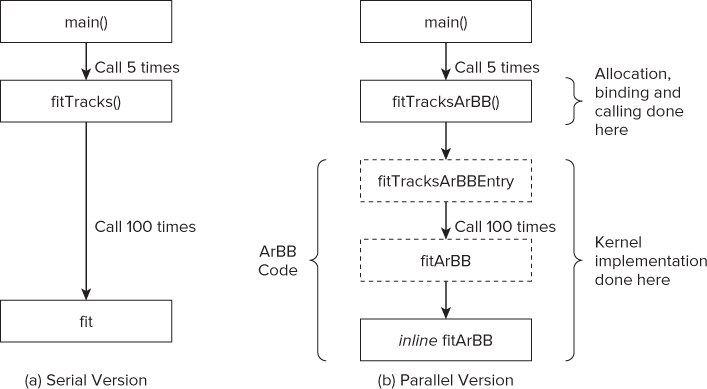
The bottom box of the parallel version contains the Kalman filter and is supplied with ArBB code already implemented. You will add all the preceding blocks in Activities 15-3 to 15-6.
As described in the first part of this case study (refer to Figure 15.8 and associated text), you should apply ArBB in four steps:
![]()
Identifying the Kernel in the Driver
The kernel, which is invoked by a call operator, contains the entire contents of the serial driver.
New Prototype
The kernel prototype has five parameters, the first three being based on the original C code, the second two being the addresses to the newly introduced ArBB containers vtT and vtC:
void fitTracksArBBEntry( i32 vSize, TracksArBB<FTYPE> vTracksArBB,
                         StationsArBB<FTYPE> vStationsArBB,
                         dense< array<FTYPE, 6> > &vtT,
                         dense< array<FTYPE, 15> > &vtC    );
New Classes
The classes for magnetic fields, stations, and tracks defined in classes.h need to be replaced with ArBB equivalents. Two new classes, StationsArBB and TracksArBB, and one structure, FieldRegionArBB, are provided for you in classes_arbb.h, and have the same member items as the original classes. However, instead of being pointers, they are ArBB containers. For example, the original class Tracks had public members:
class Tracks
{
public:
  float  *MC_x, *MC_y, *MC_z, *MC_px, *MC_py, *MC_pz, *MC_q;
  int    *nHits, *NDF;
  float  **hitsX, **hitsY;
  float  *hitsX2, *hitsY2;
  int    **hitsIsta;

  Tracks(){};
The new class, TracksArBB, reflects these members as containers:
class TracksArBB
{
public:
  dense<f32>     MC_x, MC_y, MC_z, MC_px, MC_py, MC_pz, MC_q;
  dense<i32>     nHits, NDF;
  dense<f32, 2>  hitsX, hitsY;
  dense<f32, 2>  hitsX2, hitsY2;
  dense<i32, 2>  hitsIsta;

  TracksArBB(){};
Note that within all the project files, the following type definitions have been used:
    typedef float ftype;    // set ftype to be single precision data
    typedef f32   FTYPE;    // set FTYPE to be ArBB single precision data
void fitTracksArBBEntry(…)
{
        #if 0
…
        #endif
}
void fitTracksArBBEntry( i32 vSize, TracksArBB<FTYPE> vTracksArBB,
                         StationsArBB<FTYPE> vStationsArBB,
                         dense< array<FTYPE, 6> > &vtT,
                         dense< array<FTYPE, 15> > &vtC    )
{
}
#include "classes.h"       // Main Kalman filter classes
#include "arbb_classes.h"  // Added classes for parallel driver
#include "arbb.hpp"        // Added for ArBB namespace data
nmake -f Makefile-WIN32
Allocating and Binding
Each of the new ArBB classes now needs to be instantiating, and the original data bound to this new instantiation. This binding is carried out in driver.cpp, in the function fitTracksArBB. You can try out the allocating and binding for yourself in Activity 15-4.
Binding TracksArBB and StationArBB
An instance of the old Tracks class already exists within ReadFiles.cpp, called vTracks. The member items of this class contain all the track information loaded from the data files. You must now bind these member items with the containers in the new class TracksArBB — for example:
TracksArBB<FTYPE> vTracksArBB;       // create new instance of new class
                                     // bind with existing information from
                                     // instance of old class Tracks
bind(vTracksArBB.MC_x, vTracks.MC_x, nT );
bind(vTracksArBB.MC_y, vTracks.MC_y, nT );
.  .  .  .  .  . etc
Similarly, an instance of the new class StationsArBB must be created and bound with the existing information from the instance of the old Stations class:
StationsArBB<FTYPE> vStationsArBB;   // create new instance of new class
                                     // bind with existing information from
                                     // instance of old class Stations
bind(vStationsArBB.z, vStations.z, nS );
bind(vStationsArBB.thick, vStations.thick, nS );
.  .  .  .  .  . etc
Swapping the Order of the Track
The original track hit information is held in members hitsX and hitsY. These are two-dimensional arrays with the track number first and station number last. For ArBB parallelization, which aims to simultaneously process tracks, you should store this information in reverse order, with the track number last. To facilitate this, create two new arrays, X2hits and Y2hits, into which the hit information is transferred in the correct order. In the following example code, nT and nS are the number of tracks and stations, respectively:
ARBB_CPP_ALIGN(ftype * X2hits);
ARBB_CPP_ALIGN(ftype * Y2hits);
// reserve array space
X2hits = ( ftype * ) arbb::aligned_malloc( sizeof( ftype ) * nS * nT  );
Y2hits = ( ftype * ) arbb::aligned_malloc( sizeof( ftype ) * nS * nT  );
// load hit data in reverse order
for(int ix = 0; ix < nT; ix ++)
{
  for(int jx = 0; jx < nS; jx ++)
  {
    X2hits[jx * nT + ix] = vTracks.hitsX[ix][jx];
    Y2hits[jx * nT + ix] = vTracks.hitsY[ix][jx];
  }
}
Notice the use of ArBB alignment macros and functions. You can bind these new arrays to members of the new TracksArBB class instance vTrackArBB as follows:
bind(vTracksArBB.hitsX2, X2hits, nT, nS);
bind(vTracksArBB.hitsY2, Y2hits, nT, nS);
Swapping the Order of the State and Covariance Matrices
The order of the two-dimensional state and covariance matrices T and C also need to be swapped. These are empty arrays at this point, so no actual data needs to be transferred. However, you should create new matrices of the correct order and bind them to appropriate ArBB containers. For example, the T state matrix has a new matrix, TBuf, which is bound to the container vtT:
// define a state array of 6 pointers
ARBB_CPP_ALIGN(ftype *TBuf[6]);
// reserve array space for each, size number of tracks
for( int i = 0; i < 6; i ++ )
{
  TBuf[i] = ( ftype * ) arbb::aligned_malloc( sizeof( ftype ) * nT );
}
// define array of 6 dense containers for state matrix
dense< array<FTYPE, 6>  >  vtT;
// bind to state matrix
bind(vtT, nT, TBuf[0], TBuf[1], TBuf[2], TBuf[3], TBuf[4], TBuf[5]);
You should repeat this with the 15-component covariance matrix C, where a new matrix, CBuf, needs to be created and bound with a new container, vtC.
nmake -f Makefile-WIN32
Invoking the Kernel
The kernel is invoked through a call operation. This new function is passed the ArBB-style data containers, as follows:
// set number of tracks in ArBB data type
i32 vSize = nT;
// Invoke Kalman filter track fitter by call operator
call(fitTracksArBBEntry)(vSize, vTracksArBB, vStationsArBB, vtT, vtC);
At this point in the code you can now invoke the kernel function through a call operation, as shown in step 3 of Activity 15-5.
Before returning from the fitTracksArBB function, you must store the contents of matrices TBuf and CBuf into the originally passed matrices of T and C, and release their spaces. You also need to release the space used for the X2hits and Y2hits matrices. The following snippet uses TBuf as an example:
// Store TBuf data into T matrix in desired order
for( int i = 0; i < nT; i ++ )
{
  for( int j = 0; j < 6; j ++ )
  {
    T[i][j] = TBuf[j][i];
    }
  }
  // Release memory of TBuf matrix
  for( int i = 0; i < 6; i ++ )
  {
    arbb::aligned_free( TBuf[i] );
  }
nmake -f Makefile-WIN32
Implementing the Kernel
Your last step in converting the program to use ArBB is to implement the contents of the fitTracksArBBEntry kernel function.
Calling the Parallel Kalman Filter
The new code has the same heuristics as the original serial code, applying the Kalman filter on the 20,000 tracks in a for loop iterating 100 times, and then extrapolating the start points of the tracks.
An ArBB-type _for loop is used in the first part:
_for( j = (usize)0, j < Ntimes, j ++ )
{
  fitArBB( vTracksArBB, vStationsArBB, magFieldArBB, vtT, vtC );
}_end_for;
where usize is an ArBB data type used for indices.
Finally, the extrapolation of the tracks requires you to use a local state and covariance matrices T and C, which you must load with the current values from the containers vtT and vtC. The following example uses the T state matrix:
// define local matrices of dense containers
dense<FTYPE> T[6];
dense<FTYPE> C[15];

// load T with contents of vtT
T[0] = vtT.get<FTYPE, 0>();
T[1] = vtT.get<FTYPE, 1>();
T[2] = vtT.get<FTYPE, 2>();
T[3] = vtT.get<FTYPE, 3>();
T[4] = vtT.get<FTYPE, 4>();
T[5] = vtT.get<FTYPE, 5>();
Then call the parallel version of the extrapolation function:
// Call extrapolation function
extrapolateALightArBB( T, C, vTracksArBB.MC_x, T[4], magFieldArBB );
Loading New Values Back into the C Structures
The last action is to reload the new T and C values into the containers vtT and vtC, respectively:
// Reload vtT with new contents of T
vtT.set<0>(T[0]);
vtT.set<1>(T[1]);
vtT.set<2>(T[2]);
vtT.set<3>(T[3]);
vtT.set<4>(T[4]);
vtT.set<5>(T[5]);
- Delete the #if 0 … #endif clause (and its contents) in the fitTracksArBBEntry function.
- Copy lines 174 to 187 of Listing 15.7 into the end of the fitTracksArBBEntry function.
nmake -f Makefile-WIN32
You are now ready to build and run the application, which should produce the output shown in Figure 15.20.
Figure 15.20 Results of running the ArBB version of track-fitting software
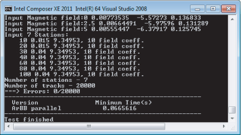
As before, after outputting some setup information involving magnetic fields and the number of stations and tracks, the timing information is given between the dashed lines. Compared to the serial timings (refer to Figure 15.17), the ArBB version is 42 times faster.
Listing 15.7: Parallel driver for the parallel version of Kalman filter track fitter
1:  #include "fit_util.h"         // a set of constants
2:  #include "classes.h"          // Main Kalman filter classes
3:  #include "arbb_classes.h"     // Added classes for parallel driver
4:  #include "arbb.hpp"           // added for arbb namespace data
5:
6:  typedef float ftype;
7:  typedef f32 FTYPE;            // Added for parallel driver
8:
9:  using namespace std;
10:  using namespace arbb;        // Access to arbb
11:
12:  // ---------------------------------- Prototypes
13:
14:
15:  void fitTracksArBBEntry( i32 vSize, TracksArBB<FTYPE> vTracksArBB,
16:                           StationsArBB<FTYPE> vStationsArBB,
17:                           dense< array<FTYPE, 6> > &vtT,
18:                           dense< array<FTYPE, 15> > &vtC    );
19:
20:  void fitArBB( TracksArBB<FTYPE> &ts, StationsArBB<FTYPE> &ss,
21:                FieldRegionArBB<FTYPE> &f,
22:                dense< array<FTYPE, 6> > &vtT,
23:              dense< array<FTYPE, 15> > &vtC   );
24:
25:void extrapolateALightArBB( dense<FTYPE> *T, dense<FTYPE> *C,
26:dense<FTYPE>
27:                            &zOut,dense<FTYPE>& qp0,
28:                            FieldRegionArBB<FTYPE> &F);
29:
30:// ------------------------- Global data, instances of classes
31:
32:extern FieldRegion     magField;
33:extern Stations        vStations;
34:extern Tracks          vTracks;
35:
36:// *** Driving ArBB Parallel Version of Kalman Filter Track Fitter ***
37:
38:void fitTracksArBB( ftype (*T)[6], ftype (*C)[15], int nT, int nS )
39:{
40:  int ix, jx;
41:
42: // -----------------------------------------------------------------
43:  // Create new arrays to hold track hits and load with track hit data.
44:  // The new data is transposed so the last index is track number,
45:  // rather than first
46:  // Create two pointers for track hit data
47:  ARBB_CPP_ALIGN(ftype * X2hits);
48:  ARBB_CPP_ALIGN(ftype * Y2hits);
49:  // reserve array space
50:  X2hits = ( ftype * ) arbb::aligned_malloc( sizeof(ftype) * nS * nT  );
51:  Y2hits = ( ftype * ) arbb::aligned_malloc( sizeof(ftype) * nS * nT  );
52:  // load hit data in reverse order
53:  for(ix = 0; ix < nT; ix ++)
54:  {
55:    for(jx = 0; jx < nS; jx ++)
56:    {
57:      X2hits[jx * nT + ix] = vTracks.hitsX[ix][jx];
58:      Y2hits[jx * nT + ix] = vTracks.hitsY[ix][jx];
59:    }
60:  }
61:
62: // ---------------------------------------------------------------
63:  // Create new temporary set of arrays for state
64:  // and covariance matrix data.
65:  // The passed T & C matricies are 2D in the wrong order,
66:  // with track number as the first index.
67:  // Define a state array of 6 pointers
68:  ARBB_CPP_ALIGN(ftype *TBuf[6]);
69:  // reserve array space for each, size number of tracks
70:  for( int i = 0; i < 6; i ++ )
71:  {
72:    TBuf[i] = ( ftype * ) arbb::aligned_malloc( sizeof( ftype ) * nT );
73:  }
74:  // define a covariance array of 15 pointers
75:  ARBB_CPP_ALIGN(ftype *CBuf[15]);
76:  // reserve array space for each
77:  for( int i = 0; i < 15; i ++ )
78:  {
79:    CBuf[i] = ( ftype * ) arbb::aligned_malloc( sizeof( ftype ) * nT );
80:  }
81:  // define array of 6 dense containers for state matrix
82:  dense< array<FTYPE, 6>  >  vtT;
83:  // bind to state matrix
84:  bind(vtT, nT, TBuf[0], TBuf[1], TBuf[2], TBuf[3], TBuf[4], TBuf[5]);
85:  // define array of 15 dense containers for covariance matrix
86:  dense< array<FTYPE, 15> >  vtC;
87:  // bind to covariance matrix
88:  bind(vtC, nT, CBuf[0], CBuf[1], CBuf[2], CBuf[3], CBuf[4], CBuf[5],
89:  CBuf[6], CBuf[7], CBuf[8], CBuf[9], CBuf[10], CBuf[11],
90:  CBuf[12], CBuf[13], CBuf[14]);
91: // ---------------------------------------------------------------
92:  // Create and bind new instances of TrackArBB and StationArBB data
93:  // create new instance of new class
94:  TracksArBB<FTYPE> vTracksArBB;
95:  // bind with existing information from
96:  // instance of old class Tracks
97:  bind(vTracksArBB.MC_x, vTracks.MC_x, nT );
98:  bind(vTracksArBB.MC_y, vTracks.MC_y, nT );
99:  bind(vTracksArBB.MC_z, vTracks.MC_z, nT );
100:  bind(vTracksArBB.MC_px, vTracks.MC_px, nT );
101:  bind(vTracksArBB.MC_py, vTracks.MC_py, nT );
102:  bind(vTracksArBB.MC_pz, vTracks.MC_pz, nT );
103:  bind(vTracksArBB.MC_q, vTracks.MC_q, nT );
104:  bind(vTracksArBB.nHits, vTracks.nHits, nT );
105:  bind(vTracksArBB.NDF, vTracks.NDF, nT );
106:  bind(vTracksArBB.hitsX, vTracks.hitsX[0], nS, nT );
107:  bind(vTracksArBB.hitsY, vTracks.hitsY[0], nS, nT );
108:  bind(vTracksArBB.hitsX2, X2hits, nT, nS);
109:  bind(vTracksArBB.hitsY2, Y2hits, nT, nS);
110:  bind(vTracksArBB.hitsIsta, vTracks.hitsIsta[0], nS, nT );
111:  // create new instance of new class
112:  StationsArBB<FTYPE> vStationsArBB;
113:  // bind with existing information from
114:  // instance of old class Stations
115:  bind(vStationsArBB.z, vStations.z, nS );
116:  bind(vStationsArBB.thick, vStations.thick, nS );
117:  bind(vStationsArBB.zhit, vStations.zhit, nS );
118:  bind(vStationsArBB.RL, vStations.RL, nS );
119:  bind(vStationsArBB.RadThick, vStations.RadThick, nS );
120:  bind(vStationsArBB.logRadThick, vStations.logRadThick, nS );
121:  bind(vStationsArBB.Sigma, vStations.Sigma, nS );
122:  bind(vStationsArBB.Sigma2, vStations.Sigma2, nS );
123:  bind(vStationsArBB.Sy, vStations.Sy, nS );
124:  bind(vStationsArBB.mapX, vStations.mapX[0], 10, nS );
125:  bind(vStationsArBB.mapY, vStations.mapY[0], 10, nS );
126:  bind(vStationsArBB.mapZ, vStations.mapZ[0], 10, nS );
127: // ---------------------------------------------------------------
128:  // Invoke call to track fitter by a call operation
129:  // set number of tracks in ArBB data type
130:  i32 vSize = nT;
131:  // Invoke Kalman filter track fitter by call operator
132:  call(fitTracksArBBEntry)(vSize,vTracksArBB,vStationsArBB,vtT,vtC);
133:
134:  // copy container to C buffers
135:  vtT.read_only_range();
136:  vtC.read_only_range();
137:
138: // --------------------------------------------------------------
139:  // Pack temporary array data back into T & C arrays, transposing
140:  // order of storage back to the original with track number being the
141:  // first index
142:  for( int i = 0; i < nT; i ++ )
143:  {
144:    for( int j = 0; j < 6; j ++ )
145:    {
146:      T[i][j] = TBuf[j][i];
147:    }
148:    for( int j = 0; j < 15; j ++ )
149:    {
150:      C[i][j] = CBuf[j][i];
151:    }
152:  }
153: // --------------------------------------------------------------
154:  // Release memory of TBuf and CBuf matrices
155:  for( int i = 0; i < 6; i ++ )
156:  {
157:    arbb::aligned_free( TBuf[i] );
158:  }
159:  for( int i = 0; i < 15; i ++ )
160:  {
161:    arbb::aligned_free( CBuf[i] );
162:  }
163:
164:  arbb::aligned_free( X2hits );
165:  arbb::aligned_free( Y2hits );
166:}
167:
168://******************************************************************
169:void fitTracksArBBEntry( i32 vSize, TracksArBB<FTYPE> vTracksArBB,
170:                                    StationsArBB<FTYPE> vStationsArBB,
171:                                    dense< array<FTYPE, 6> > &vtT,
172:                                    dense< array<FTYPE, 15> > &vtC   )
173:{
174:  // create a FieldRegion class instance
175:  FieldRegionArBB<FTYPE> magFieldArBB(vSize);
176:  // create an ArBB index type
177:  usize j;
178:
179: // -------------------------------------------------------------
180:  // Repeat 100 times the call to the
181:  // Kalman filter Track fitter
182:  // Using ArBB type for loop
183:  _for( j = (usize)0, j < Ntimes, j ++ )
184:  {
185:    fitArBB( vTracksArBB, vStationsArBB, magFieldArBB, vtT, vtC );
186:  }_end_for;
187:
188: // -------------------------------------------------------------
189:  // Extrapolate to start of tracks as in serial version
190:  // define local matrices of dense containers
191:  dense<FTYPE> T[6];
192:  dense<FTYPE> C[15];
193:  // load T with contents of vtT
194:  T[0] = vtT.get<FTYPE, 0>();
195:  T[1] = vtT.get<FTYPE, 1>();
196:  T[2] = vtT.get<FTYPE, 2>();
197:  T[3] = vtT.get<FTYPE, 3>();
198:  T[4] = vtT.get<FTYPE, 4>();
199:  T[5] = vtT.get<FTYPE, 5>();
200:
201:  // load C with contents of vtC
202:  C[0] = vtC.get<FTYPE, 0>();
203:  C[1] = vtC.get<FTYPE, 1>();
204:  C[2] = vtC.get<FTYPE, 2>();
205:  C[3] = vtC.get<FTYPE, 3>();
206:  C[4] = vtC.get<FTYPE, 4>();
207:  C[5] = vtC.get<FTYPE, 5>();
208:  C[6] = vtC.get<FTYPE, 6>();
209:  C[7] = vtC.get<FTYPE, 7>();
210:  C[8] = vtC.get<FTYPE, 8>();
211:  C[9] = vtC.get<FTYPE, 9>();
212:  C[10] = vtC.get<FTYPE, 10>();
213:  C[11] = vtC.get<FTYPE, 11>();
214:  C[12] = vtC.get<FTYPE, 12>();
215:  C[13] = vtC.get<FTYPE, 13>();
216:  C[14] = vtC.get<FTYPE, 14>();
217:
218:  // Call extrapolation function within the filter
219:  extrapolateALightArBB( T, C, vTracksArBB.MC_x, T[4], magFieldArBB );
220:
221:  // Reload vtT with new contents of T
222:  vtT.set<0>(T[0]);
223:  vtT.set<1>(T[1]);
224:  vtT.set<2>(T[2]);
225:  vtT.set<3>(T[3]);
226:  vtT.set<4>(T[4]);
227:  vtT.set<5>(T[5]);
228:
229:  // Reload vtC with new contents of C
230:  vtC.set<0>(C[0]);
231:  vtC.set<1>(C[1]);
232:  vtC.set<2>(C[2]);
233:  vtC.set<3>(C[3]);
234:  vtC.set<4>(C[4]);
235:  vtC.set<5>(C[5]);
236:  vtC.set<6>(C[6]);
237:  vtC.set<7>(C[7]);
238:  vtC.set<8>(C[8]);
239:  vtC.set<9>(C[9]);
240:  vtC.set<10>(C[10]);
241:  vtC.set<11>(C[11]);
242:  vtC.set<12>(C[12]);
243:  vtC.set<13>(C[13]);
244:  vtC.set<14>(C[14])
245:}
code snippet Chapter1515-7.cpp
Summary
This case study was used as an introduction to ArBB. Starting with a serial version of the track-fitting application, the program was altered in many steps before finally producing a parallel version.
ArBB is an excellent parallelism tool for programs that are heavily data-centric. Its containers, pseudo data objects that can be bound to existing C/C++ data, allow calculations through the use of simple mathematical operators between them. The ArBB libraries overlay complex operations between arrays and matrices (even of different sizes) as if they were single variables.
As a programmer, you are not explicitly responsible for any parallelization in ArBB. This means data races and other such problems that can occur due to parallelization are eliminated. ArBB's methods also ensure a balanced load between the threads of a parallel program.
Because of the JIT compiler, ArBB “future-proofs” your application against new CPU architectures. When an ArBB function is first called, the JIT compiler generates code tuned to its runtime environment.
Chapter 16, “Parallelizing Legacy Code,” looks at some of the issues you might face when parallelizing old code. Using the Dhrystone benchmark, the code is made parallel using OpenMP and Cilk Plus.