
Chapter 9
Tuning Parallel Applications
What's in This Chapter?
Using Amplifier XE to profile a parallel program
The five tuning steps
Using the Intel Software Autotuning Tool
Chapters 6–8 described the first three steps to make your code parallel — analyze, implement, and debug. This chapter discusses the final challenge — tuning your parallel application so that it is load-balanced and runs efficiently.
The chapter begins by describing how to use Amplifier XE to check the concurrency of your parallel program, and then shows how to detect and tune any synchronization problems. The chapter concludes by describing the experimental Intel Software Autotuning Tool (ISAT).
Note that all the screenshots and instructions in this chapter are based on Windows XE; however, you can run the hands-on activities on Linux, as well.
Introduction
Amplifier XE provides two predefined analysis types to help tune your parallel application:
- Concurrency analysis — Use this to find out which logical CPUs are being used, to discover where parallelism is incurring synchronization overhead, and to identify potential candidates for further parallelization.
- Locks and Waits analysis — Use this to identify where your application is waiting on synchronization objects or I/O operations, and to discover how these waits affect your program performance.
In this chapter, you use the Concurrency analysis as the main vehicle for parallel tuning. If your program has a lot of synchronization events, you may find the Locks and Waits analysis useful. Because both of these analysis types run in user mode, you can use them on both Intel and non-Intel processors.
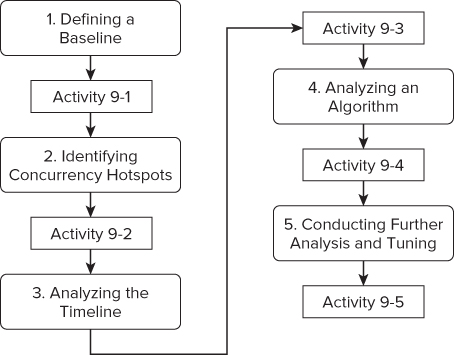
Figure 9.1 shows the different tuning steps carried out in this chapter. You should have already fixed any data races and deadlocks (refer to Chapter 8, “Checking for Errors”) before starting to tune your parallel application.
Figure 9.1 The five steps for tuning parallel applications
Defining a Baseline
The first step to undertake for any performance tuning is to create a baseline to compare against. Ideally, the baseline test should give the same results each time you run it; otherwise, it would be very difficult to be certain that an improvement in performance is not just due to some random behavior of your program or system.
Ensuring Consistency
If the program you are testing gives wildly different results, try the following:
- Turn off Turbo Boost, speed-step, and hyper-threading in the BIOS of your computer (but do not turn off multi-core support). These options can cause huge variations from one run to the next of your program. For more discussion on this point, see Chapter 4, “Producing Optimized Code.” Once you have finished performance tuning, you should remember to turn these features back on.
- If possible, disable any antivirus software. If this is not possible, run your program twice after each rebuild. Often the antivirus software will kick in only on the first run of a program.
- Run the program more than once, and take an average result of any timing values.
Measuring the Performance Improvements
When tuning parallel programs you need to keep an eye on two things:
- The total time the program runs (assuming time taken is the key performance measure).
- Performance improvements of the parallel part of the program within your code.
In the prime numbers example used in this chapter (ParallelPrime.cpp, from Listing 9.4 at the end of the chapter), three different timing values are available:
- The time it takes to calculate the prime numbers, as printed out in the program.
- The elapsed time, as recorded by Amplifier XE.
- The time taken to execute the parallel region, as recorded by Amplifier XE.
Most of the time you should concentrate on performance improvements of the parallel region, but remember to keep an eye on the other figures as well.
Measuring the Baseline Using the Amplifier XE Command Line
You can use the command-line version of Amplifier XE to profile your code and produce a report. If you like, you can then look at the results generated from the command line with the GUI version of Amplifier XE.
In Activity 9-1 you build and test a program that calculates prime numbers. The program has been parallelized using the OpenMP method. Once the test program has been built, the following command produces a concurrency report, which in this case is the result of running the application on a 12-core machine. Your report may be different.
amplxe-cl -collect concurrency ./9-1.exe
100%
Found     13851 primes in  7.7281 secs
Using result path ‘C:CH9
000cc’
Executing actions 75 % Generating a report
Summary
-------

Average Concurrency:  0.975
Elapsed Time:         8.028
CPU Time:             55.051
Wait Time:            85.423
Executing actions 100 % done
You can see that:
- The Average Concurrency — the measure of how many threads were running in parallel — is very poor. In fact, the program has effectively been serialized.
- The Elapsed Time — the total time for the program to run — was just over eight seconds. This includes a slight overhead introduced by the act of profiling.
- The program has more Wait Time than CPU Time. Wait Time is the amount of time the threads are waiting for a resource. CPU Time is the sum of the time each core has spent executing code.
You can use the Amplifier XE command-line interface to generate a hotspot report. The example shown in Figure 9.2 generates a hotspot report, with the results grouped by openmp-task. This is a convenient way of seeing how much time the parallel for loop (in lines 51–60 of ParallelPrime.cpp) took.
Figure 9.2 A command line hotspot report
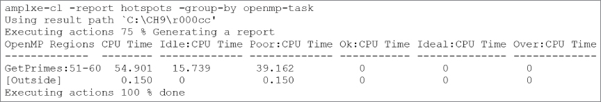
Notice that no results folder is passed to Amplifier XE, which causes Amplifier XE to use the most recently generated results.
From the results, you can see the following:
- The parallel region consumes most of the execution time of the program. This is good; it means that any improvement you make in the parallel section of the code will positively impact the performance of the whole program.
- The concurrency rate of the parallel region is Poor. A well-tuned parallel program should have a concurrency of at least OK.
- For 20 percent of the time, the parallel region is Idle. A well-tuned parallel program ideally should have no Idle time.
Building and Running the Program
Windows
icl /O2 /Zi /Qopenmp /Ob1 ParallelPrime.cpp wtime.c -o 9-1.exe
Linux
icc -O2 -g -openmp -inline-level=1 ParallelPrime.cpp wtime.c -o 9-1.exe
The option /Zi (-inline-level=1)
9-1.exe
#define LAST 300000
Using the Command-Line Version of Amplifier XE to Get a Timestamp
amplxe-cl -collect concurrency ./9-1.exe
amplxe-cl -report hotspots -group-by openmp-task
Identifying Concurrency Hotspots
Having created a baseline of your parallel application, you can start looking at the performance in more detail by examining how well the program is using the CPU cores. You can try this out for yourself in Activity 9-2.
Thread Concurrency and CPU Usage
Thread concurrency and CPU usage will help you get a good feel for how parallel your program is.
- Thread concurrency is a measure of how many threads are running in parallel. Ideally, the number of threads running in parallel should be the same as the number of logical cores your processor can support.
- CPU usage measures how many logical cores are running simultaneously.
Figure 9.3 shows the thread concurrency of the application when it is run on a 12-core Windows-based workstation. As you can see, it runs with a low concurrency, with most of the time no threads running concurrently. The concurrency information is split into four regions — Poor, OK, Ideal, and Over — and are colored red, orange, green, and blue, respectively (albeit not shown in the figure). You can change the crossover point between each region by highlighting and dragging the triangular shaped cursors that are positioned just below the horizontal bar.
Figure 9.3 Concurrency of the Windows application
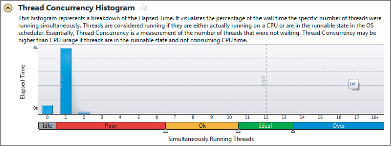
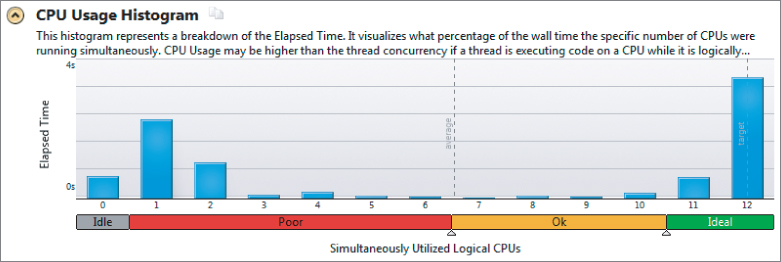
Figure 9.4 shows the CPU usage of the baseline program on Windows. It shows the length of time when various numbers of CPUs were running concurrently. For example, for almost a second no CPUs were running, and for approximately 1.3 seconds two CPUs were running concurrently. Ideally, there would be a single entry showing 12 CPUs running all the time. In this case you can see that not all the CPUs were in use all the time. The dotted vertical line indicates that the average concurrent CPU usage is almost 7.
Figure 9.4 CPU usage of the Windows application
Identifying Hotspots in the Code
The Bottom-up view of the analysis shows the main hotspots in the system (see Figure 9.5).
Figure 9.5 Source code view of CPU usage
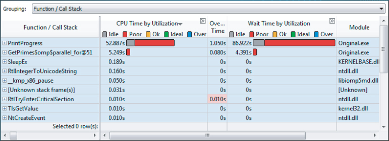
The largest hotspot is the PrintProgress function, with most of the bar colored red. When you tune any parallel code, your goal is to get the colored bar to be green, indicating that the concurrency is ideal.
Double-clicking the hotspot brings up the Source view of the hotspot (see Figure 9.6).
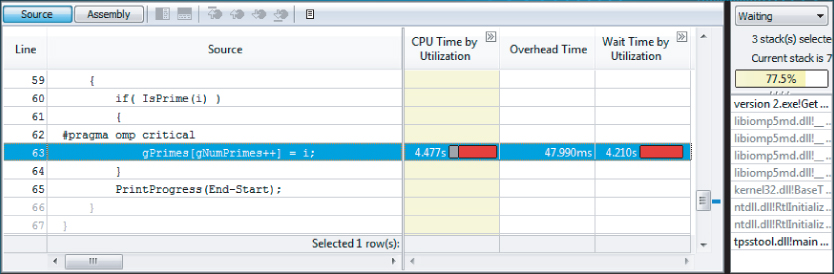
Figure 9.6 The biggest hotspot in the code
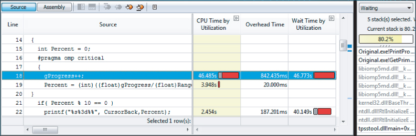
Notice the following:
- The PrintProgress function has three hotspots, at lines 18, 19, and 22. Line 18 is the biggest hotspot, with a CPU Time of just over 46 seconds.
- Lines 18 and 22 have significant amounts of Wait Time by Utilization. This is discussed more in the section “Analyzing the Timeline.”
- The stack pane (on the right) reports five stacks, and that the current stack contributes to 80.2% of the hotspot. If you toggle through the five stacks, by clicking the arrow (next to “1 of 5”), the other stacks are reported as contributing 10.1%, 7.6%, 2.0%, and 0.1%. In this program, the call stack information is not needed for tuning purposes, but you may find it useful when you analyze other programs.
amplxe-gui r000cc
- Highlight a small part of the timeline.
- Right-click and select Zoom in on Selection.
- Repeat these steps until you can see about a dozen or so transitions.
- Hover the mouse over some of the transition lines and identify which type of transition is occurring.
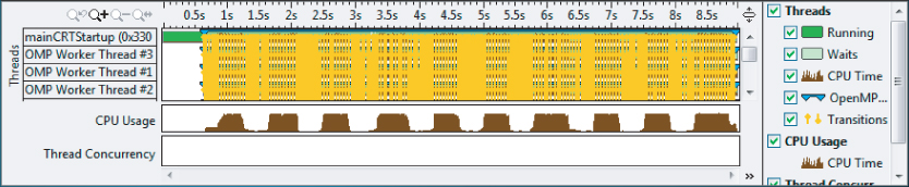
Analyzing the Timeline
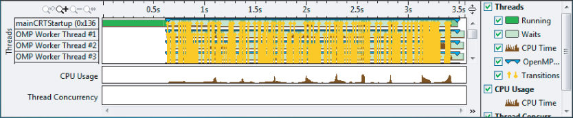
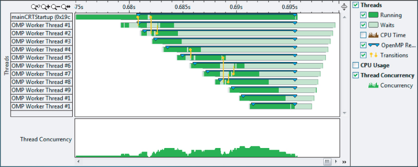
You can use the timeline of an analysis to better understand how your program is behaving. Figure 9.7 shows the timeline of the baseline application. You can glean further information about the program from four distinct areas of the display:
- In the list of threads (the left-hand side) are twelve OpenMP worker threads plus one master thread. Not all the worker threads are displayed, but you can see them by either scrolling down or resizing the timeline pane.
- Each horizontal bar gives more information about the runtime behavior of each thread. You can see when a thread is running or waiting. A running thread is colored dark green, and a waiting thread is colored light green. You can also see the transitions between threads. There are so many transitions that the whole of the timeline appears as a solid block of yellow. You can always turn the transitions off by unchecking its box on the right.
- The CPU Usage chart shows that most of the CPUs are used all the time, but nine rather interesting dips where the CPU usage drops dramatically.
- The Thread Concurrency bar is empty (that is, no concurrency). It seems that for most of the time, the program is running serially — a fact you already know from the summary analysis.
Figure 9.7 The application timeline
Questions to Answer
From the information in the timeline, you need to answer three questions:
- Why are there so many transition lines?
- Why is the concurrency so poor?
- What is the cause of the dips in the CPU usage?
The last question is answered in the section, “Analyzing an Algorithm.”
When you analyze your own programs, you may see other patterns that need more exploration. The important thing is that you make sure you understand all the patterns you see.
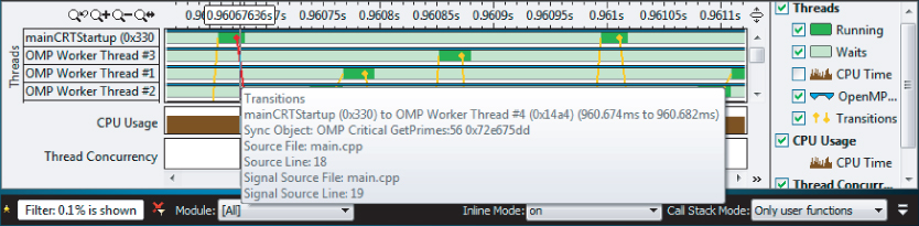
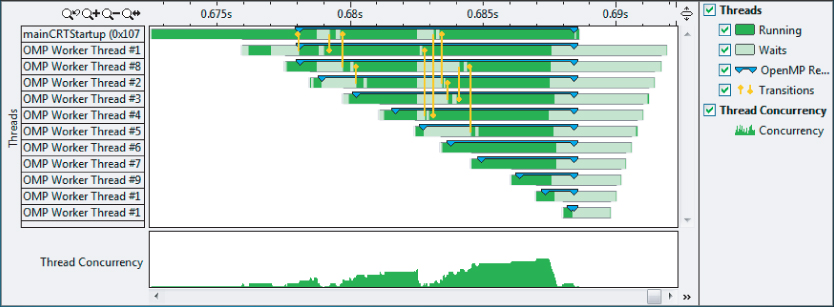
The poor concurrency and the reason for the many transition lines can be deduced from a zoomed-in view of the timeline (see Figure 9.8). There is only ever one thread running at any time; the other threads are waiting. Between each thread is a transition line. If you hover your mouse over a transition line, details about that transition are displayed (as in the figure), which show that a critical section is involved.
Figure 9.8 Zooming in on the transitions
Fixing the Critical Section Hotspot
If you double-click the transition line, the source code of the object is displayed (the same source code that you have already seen in Figure 9.6).
The #pragma omp critical construct is used to protect the reading and writing of the gProgress shared variable that is being incremented. Without the critical section, there would be a data race. A variable can be incremented much more efficiently by using an atomic operation.
The following code shows how you can use the #pragma omp atomic construct to protect the incrementing of gProgress. The reading of gProgress at line 19 does not need protecting, because a data race occurs only when there are unsynchronized reads and writes. Reading shared variables will not cause data races.
// old code
16:  #pragma omp critical
17:  {
18:    gProgress++;
19:    Percent = (int)((float)gProgress/(float)Range *200.0f + 0.5f);
20:  }

// new code
16:  #pragma omp atomic
17:  gProgress++;
18:
19:  Percent = (int)((float)gProgress/(float)Range *200.0f + 0.5f);
20:
With the fix in place, running a new analysis shows an improvement, as shown in Table 9.1. The program now has a much shorter elapsed time, and the CPU time used in the parallel part of the code has reduced by a factor of almost eight. You can try out Activity 9-3 to see these results for yourself. Often solving simple problems involving just a few of the many lines of program's code can result in large improvements in its operation.
amplxe-gui r000cc
16:  #pragma omp atomic
17:  gProgress++;
18:
19:  Percent = (int)((float)gProgress/(float)Range *200.0f + 0.5f);
20:
Table 9.1 The Results of Replacing the Critical Section with an Atomic Operation
| Metric | Original | With Atomic |
| Average Concurrency | 0.975 | 0.715 |
| Elapsed Time | 8.028 | 2.777 |
| CPU Time | 55.051 | 7.441 |
| Wait Time | 85.423 | 28.418 |
| Parallel Region CPU Time | 54.901 | 7.090 |
| Parallel Region Idle Time | 15.739 | 3.432 |
In the next step, you explore the dips in the CPU usage, which look like they might be caused by a flaw in the algorithm of the program.
Analyzing an Algorithm
In Figure 9.7 you saw nine distinct dips in the CPU usage. Once you have fixed the data race by adding the #pragma omp atomic, the dips are less pronounced but are still clearly visible (see Figure 9.9).
Figure 9.9 The timeline after the atomic operation has been introduced
To see what is causing the dips, zoom in and filter on the timeline (see Figure 9.10). Notice that the call stack mode on the bottom right has been set to user + 1 so that the function calling the hotspot is also displayed. You can see that the hotspot is the printf function, which has a high Wait Time by Utilization. Notice that all the threads are mostly light green, indicating that they are in a waiting state, with just OMP Worker Thread #4 showing some activity in the middle of the timeline.
Figure 9.10 Examining the CPU usage dips
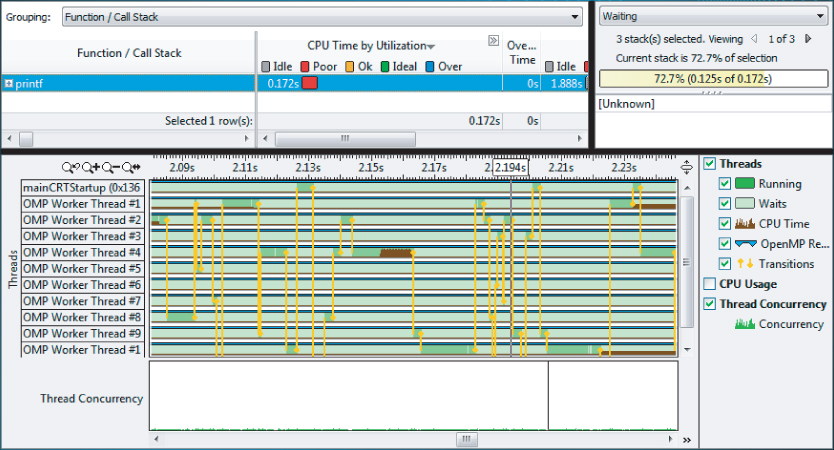
Looking at the code that calls printf in the function PrintProgress, you can see that whenever the percent value is a multiple of 10, printf is called:
21:   if( Percent % 10 == 0 )
22:     printf("%s%3d%%", CursorBack,Percent);
The intention is to display the progress on the screen after each 10 percent increment of work.
Looking at the length of the timeline, you can see that it has a length of approximately 0.13 seconds — an awfully long time to do one printf! You should suspect that something is wrong with this code and is causing the nine dips in CPU usage.
When you find a section of code that may be causing a problem, one quick test you can try is to comment out the code and see what difference it makes. Figure 9.11 shows the timeline of the application with lines 21 and 22 commented out. You can see that the dips in CPU usage have disappeared, confirming that lines 21 and 22 were the cause.
Figure 9.11 The application timeline with the printf removed
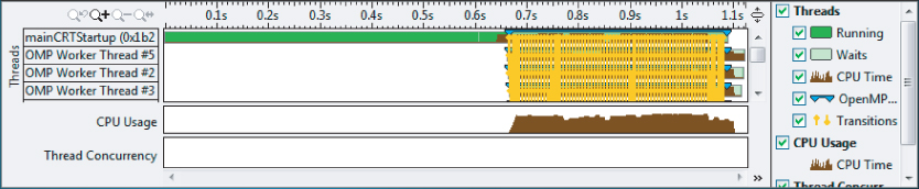
Amplifier XE will not tell you how to fix problems with your program algorithms, but it will let you observe any odd behavior.
In lines 21 and 22, the problem is caused because the printf is not only called when you first reach a percent value that is divisible by ten, but that it is then repeatedly called until Percent % 10 == 0 evaluates to false.
By modifying the code to look like Listing 9.1 (as you'll do in Activity 9-4), printf should be called only once on each 10 percent increment; the changes to the code are highlighted:
 Listing 9.1: The modified PrintProgress function
12:  // Display progress
13: void PrintProgress(int Range )
14: {
15:   int Percent = 0;
16:   static int lastPercentile = 0;
17:   #pragma omp atomic
18:   gProgress++;
19:   Percent = (int)((float)gProgress/(float)Range *200.0f + 0.5f);
20:   if( Percent % 10 == 0 )
21:   {
22:     // we should only call this if the value is new!
23:     if(lastPercentile < Percent / 10)
24:     {
25:       printf("%s%3d%%", CursorBack,Percent);
26:       lastPercentile++;
27:     }
28:   }
29: }
code snippet Chapter99-1.cpp
Examining the CPU Utilization Dip
amplxe-gui r000cc
- Select one of the dips in the CPU utilization.
- Right-click and select Zoom in and Filter by Selection.
- Change the call stack mode (see bottom right of screen) to user “functions + 1.”
Correcting the Problem
amplxe-gui r000cc
Conducting Further Analysis and Tuning
You've already carried out some analysis of the code and fixed two programming problems. With the two problems in PrintProgress fixed, a new Concurrency analysis will reveal a different part of the code GetPrimes$omp$parallel_for@57 as the biggest concurrency hotspot (see Figure 9.12).
Figure 9.12 The new concurrency hotspot
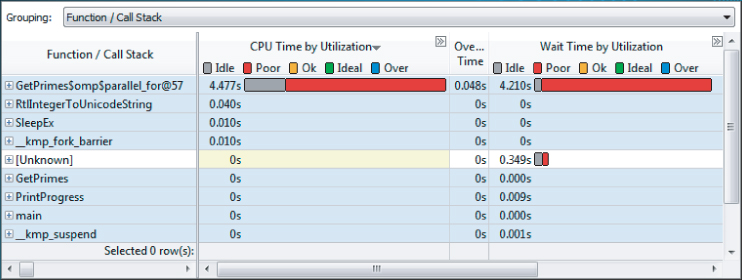
Double-clicking the hotspot GetPrimes$omp$parallel_for@57 in the Bottom-up page reveals that the hotspot is in a critical section in the function GetPrimes, as shown in Figure 9.13. Notice that the line numbers in the figure no longer match those of Listing 9.4 due to the changes made in previous sections. The GetPrimes function increments through every even number between a Start value and an End value, and tests to see if each number is a prime number by calling the IsPrime function.
Figure 9.13 Source code of the new concurrency hotspot
The critical section is applied to line 57, where the global variable gNumPrimes is incremented, and then used as an index so that the current prime (held in the variable i) can be stored into the global array gPrimes.
By now you should know what you can do to fix this — use an atomic instruction instead of the #pragma omp critical. By splitting the line into two lines, you can apply a #pragma omp critical to the incrementing of gNumPrimes:
// old code
56:       #pragma omp critical
57:       gPrimes[gNumPrimes++] = i;

// new code
56:       #pragma omp atomic
57:       gNumPrimes++;
58:       gPrimes[gNumPrimes] = i;
After you implement this code, a new analysis shows a further improvement in performance. Table 9.2 shows the performance improvement of the parallel region over the last three code changes that have been made.
Table 9.2 Performance Improvements
| Version | Time in Parallel Region (Seconds) | Comments |
| Original | 8.308 | |
| #1 | 2.847 | Replaced critical with atomic in PrintProgress |
| #2 | 0.403 | Rewrote PrintProgress |
| #3 | 0.015 | Replaced critical with atomic in GetPrimes |
Figure 9.14 shows the timeline of the parallel region. The darker part of the horizontal bars represents the time that the threads are running. Each of the start and end points of the thread are staggered; when you see such a pattern, it probably means there is scope for further tuning.
Figure 9.14 Timeline of the parallel region before tuning
You can use a schedule clause with the #pragma parallel for to try to improve the load balancing. (The schedule clause was discussed in Chapter 7, “Implementing Parallelism.”)
Most developers experiment with the different schedule clauses, keeping the one that produces the best results. Listing 9.2 shows a new listing of the GetPrimes function with the previous changes and the schedule clause added. The ISAT tool was used to find the best combination of schedule type and chunk size. You'll read more about ISAT later in this chapter.
Listing 9.2: The GetPrimes function with the schedule clause
void GetPrimes(int Start, int End)
{
  // Make Start to always be an even number
  Start += Start %2;

  // If Start is 2 or less, then just record it
  if(Start<=2) gPrimes[gNumPrimes++]=2;

  #pragma omp parallel for schedule(guided,512) num_threads(12)
  for( int i = Start; i <= End; i += 2 )
  {
    if( IsPrime(i) )
    {
      #pragma omp atomic
      gNumPrimes++;
      gPrimes[gNumPrimes] = i;
    }
    PrintProgress(End-Start);
  }
}
code snippet Chapter99-2.cpp
Figure 9.15 shows the results of the schedule clause. Note the following:
- All the threads stop running at about the same time.
- The length of the parallel region is now shorter (0.010 seconds compared with 0.015 seconds).
- The start of the threads is still staggered. Between each thread starting there is about a 1ms delay (0.001 seconds). This is probably a feature of the OpenMP run time that cannot be changed.
Figure 9.15 Timeline of the parallel region after tuning
Using Other Viewpoints
The only analysis type you have used so far is the Concurrency analysis. Within this analysis you can change the viewpoint to see the information captured with differing emphasis.
Figure 9.16 shows the viewpoints available:
- Hotspots
- Hotspots by CPU Usage
- Hotspots by Threading Concurrency
- Locks and Waits
Figure 9.16 The menu to switch viewpoints
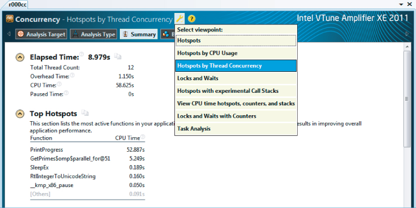
You can access this menu by clicking on the spanner icon. In your version of Amplifier XE, additional viewpoints may be available.
Using Locks and Waits Analysis
In addition to changing viewpoints, you can use other analysis types. Using the Locks and Waits analysis will give you slightly more information than a locks and waits viewpoint available from the Concurrency analysis.
Here's an example of running the Locks and Waits analysis from the command line:
amplxe-cl -collect locksandwaits ./9-1.exe
100%
Found     13851 primes in  7.6617 secs
Using result path ‘C:dvCH9Release
001lw’
Executing actions  0 % Finalizing results
Executing actions 75 % Generating a report
Summary
-------

Average Concurrency:  0.912
Elapsed Time:         7.940
CPU Time:             53.586
Wait Time:            85.153
Executing actions 100 % done
Once you have run the Locks and Waits analysis, you can view the results using the GUI version of Amplifier XE:
amplxe-gui r001lw
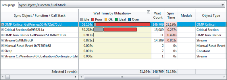
Figure 9.17 shows the analysis of the application in Listing 9.4 (without all the corrections you made earlier) using the Locks and Waits analysis. One of the differences between this analysis and a Concurrency analysis is that the hotspots are presented using synchronization objects. The first two synchronization objects listed are both critical sections. Notice that the Spin Times of the first four objects are shaded. A spinning thread is one that is executing code in a tight loop, waiting for some resource to become available. While the thread is spinning it is consuming CPU time, but it is not doing any useful work. Amplifier XE shades the values to warn you that the values are unacceptably high.
Figure 9.17 The hotspots of a Locks and Waits analysis
Other Analysis Types
You can also use other analysis types to help tune your application. Apart from the user analysis types mentioned in this chapter, you can also use Hotspot analysis (described in Chapter 6, “Where to Parallelize”) and event-based sampling (described in Chapter 12, “Event-Based Analysis with VTune Amplifier XE”).
Analyzing the New Hotspot
// old code
56:       #pragma omp critical
57:       gPrimes[gNumPrimes++] = i;
// new code
56:       #pragma omp atomic
57:       gNumPrimes++;
58:       gPrimes[gNumPrimes] = i;
amplxe-gui r001cc
Tuning the OpenMP Parallel Loop
amplxe-gui r002cc
- The running threads finish at about the same time.
- The execution time of the parallel section is shorter than you saw in step 7.
Using the Intel Software Autotuning Tool
The Intel Software Autotuning Tool (ISAT) is an experimental tool that you can use to automatically tune Cilk, OpenMP, and TBB parallel code. You can download the tool from http://software.intel.com/en-us/articles/intel-software-autotuning-tool. At the time of this writing, ISAT is available only for use in a Linux environment, although it may eventually be available for Windows as well.
ISAT works by automatically searching for the optimal values of program parameters that have a significant impact on parallel performance. Parameters include scheduling policy and granularity within the OpenMP method, task granularity within the TBB method, and cache blocking factors in matrix-intensive applications.
You control which code should be tuned by inserting directives in the form of pragmas within your existing code.
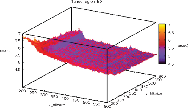
ISAT produces two outputs:
- Source code with the best scheduling parameters automatically added
- A graph of all the results (see Figure 9.18)
Figure 9.18 Visualization of ISAT results
Listing 9.3 shows the ISAT profiling pragmas added to the ParallelPrime.cpp code. The first pragma, #pragma isat tuning scope…, tells ISAT the names of the start and end of the code to be tuned (M_begin and M_end, respectively). The three variables in the pragma set the range of values to use for the schedule type, chunk size, and number of threads. For more information, refer to the help that is distributed with ISAT.
Listing 9.3: The code with ISAT macros added
// NOTE: this pragma is written on ONE line
#pragma isat tuning scope(M_begin, M_end) measure(M_begin, M_end)
variable(@omp_schedule_type, [static,dynamic,guided])
variable(@omp_schedule_chunk, range(5, 10, 1, pow2))
variable(@omp_num_threads, range(1, $NUM_CPU_THREADS, 1)) search(dependent)

// go through all numbers in range and see which are primes
void GetPrimes(int Start, int End)
{
  // Make Start to always be an even number
  Start += Start %2;

  int Range = End - Start;
  // if start is 2 or less, then just record it
  if(Start<=2) gPrimes[gNumPrimes++]=2;

  #pragma isat marker M_begin
  #pragma omp parallel for
  for( int i = Start; i <= End; i += 2 )
  {
    if( IsPrime(i) )
    {
      #pragma omp atomic
      gNumPrimes++;

      gPrimes[gNumPrimes] = i;
    }
    PrintProgress(Range);
  }
  #pragma isat marker M_end
}
code snippet Chapter99-3.cpp
Source Code
Listing 9.4 is a badly tuned implementation of a parallel program that calculates the number of primes between two values, FIRST and LAST. As the values are calculated, the program prints a status message. The message is updated in 10 percent intervals. Listing 9.5 is a timing utility used to measure how long the program takes.
Listing 9.4: A parallel program to calculate prime numbers
1:  #include <stdio.h>
2:  #include <math.h>
3:  extern "C" double wtime();
4:  #define FIRST 1
5:  #define LAST 300000
6:  #define CursorBack ""
7:  // globals
8:  int gProgress  = 0;
9:  int gNumPrimes = 0;
10: int gPrimes[10000000];
11:
12:  // Display progress
13: void PrintProgress(int Range )
14: {
15:   int Percent = 0;
16:   #pragma omp critical
17:   {
18:     gProgress++;
19:     Percent = (int)((float)gProgress/(float)Range *200.0f + 0.5f);
20:   }
21:   if( Percent % 10 == 0 )
22:     printf("%s%3d%%", CursorBack,Percent);
23: }
24:
25: // Test to see if a number is a prime
26: bool IsPrime(int CurrentValue)
27: {
28:   int Limit, Factor = 3;
29:
30:   if( CurrentValue == 1 )
31:     return false;
32:   else if( CurrentValue == 2 )
33:     return true;
34:
35:   Limit = (long)(sqrtf((float)CurrentValue)+0.5f);
36:   while( (Factor <= Limit) && (CurrentValue % Factor))
37:     Factor ++;
38:
39:   return (Factor > Limit);
40: }
41:
42: // Go through all numbers in range and see which are primes
43: void GetPrimes(int Start, int End)
44: {
45:   // Make Start to always be an even number
46:   Start += Start %2;
47:
48:   // If start is 2 or less, then just record it
49:   if(Start<=2) gPrimes[gNumPrimes++]=2;
50:
51:   #pragma omp parallel for
52:   for( int i = Start; i <= End; i += 2 )
53:   {
54:     if( IsPrime(i) )
55:     {
56:       #pragma omp critical
57:       gPrimes[gNumPrimes++] = i;
58:     }
59:     PrintProgress(End-Start);
60:   }
61: }
62:
63: int main()
64: {
65:   double StartTime = wtime();
66:   GetPrimes(FIRST, LAST);
67:   double EndTime = wtime();
68:
69:   printf("
Found  %8d primes in %7.4lf secs
",
70:       gNumPrimes,EndTime - StartTime);
71: }
code snippet Chapter9ParallelPrime.cpp
Listing 9.5: A function to find the current time
#ifdef _WIN32
#include <windows.h>
double wtime()
{
  LARGE_INTEGER ticks;
  LARGE_INTEGER frequency;
  QueryPerformanceCounter(&ticks);
  QueryPerformanceFrequency(&frequency);
  return (double)(ticks.QuadPart/(double)frequency.QuadPart);
}
#else
#include <sys/time.h>
#include <sys/resource.h>
double wtime()
{
  struct timeval time;
  struct timezone zone;
  gettimeofday(&time, &zone);
  return time.tv_sec + time.tv_usec*1e-6;
}
#endif
code snippet Chapter9wtime.c
Summary
This chapter showed how you can use Amplifier XE to help tune a parallel program. Using Amplifier XE's predefined analysis types, you can quickly find out how much concurrency your program exhibits and observe how well any synchronization objects are performing.
The examples in the chapter used OpenMP, but you can use Amplifier XE to profile Cilk Plus, TBB, and native threading code as well.
The next chapter shows how to model parallelism in your code using Intel Parallel Advisor.