
Chapter 13
The World's First Sudoku “Thirty-Niner”
What's in This Chapter?
Lars Peters Endresen and Håvard Graff, two talented engineers from Oslo, share how they created what may be the world's first Sudoku puzzle that has 39 clues
A hands-on exercise that mimics some of the programming techniques they used
This case study solves an intriguing problem: finding a Sudoku puzzle with 39 clues using the latest hardware advances. Multiple execution units, together with multiple cores, enable the modern programmer to tackle engineering problems that in the past would have been doable only on a supercomputer.
This case study uses the Streaming SIMD Extensions (SSE) registers and instructions in an ingenious way. The tricks used here can easily be used in other projects. The code is first optimized to run on one core, and then parallelism is introduced so that the code runs on several cores.
The Sudoku Optimization Challenge
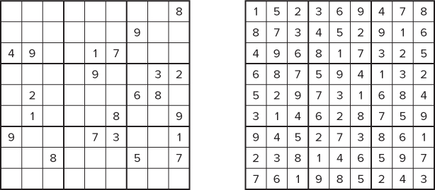
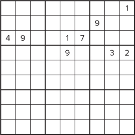
Sudoku is a number-placement puzzle that uses a 9 × 9 grid of squares into which the numbers 1 through 9 are placed. The grid is further subdivided into 3 × 3 boxes, within each of which are 3 × 3 cells. The puzzle starts with an almost empty grid with some of the cells already filled. The aim of the puzzle is to fill the grid so that every row, every column, and every 3 × 3 box contains the numbers 1 through 9. This implicitly means that no row, column, or box can have duplicated numbers within it (see Figure 13.1).
Figure 13.1 Starting and solved grids for a typical Sudoku puzzle
The challenge Endresen and Graff faced was how to generate a puzzle with 39 clues — one with 38 clues having already been produced by others. Generating Sudoku puzzles using software may seem like an easy exercise, requiring the following steps:
However, if you were to follow this approach, you would soon discover that the total number of puzzles that have to be processed makes the task almost impossible to achieve because of the length of time it would take to iterate through every possible solution.
The Nature of the Challenge
More than 6 ∞ 1021 different valid Sudoku boards exist. If a developer were to use brute force to try all the combinations of numbers, the programming exercise would be quite easy. However, the algorithm would require the lifetime of the programmer to complete the calculations. It has been estimated that a brute-force approach to producing a valid “thirty-niner” would take approximately 150 years to complete. This time can be reduced to something approaching a month by applying a number of strategies to produce an optimized version of the generator.
Four strategies are used to slim down the execution time:
- Use an algorithm that finds shortcuts through the brute-force approach by starting with a partially constructed board.
- Modify the code to take advantage of the enhanced execution units available in most of today's CPUs.
- Add parallelism to the code.
- Enable the generator to be dispatched across a cluster of machines.
The following sections go deeply into the first strategy. Although applied to Sudoku, these same strategies can be applied to a programmer's own complex algorithms in a similar fashion. Techniques learned here will enable programmers to produce fast, optimized code.
A number of other programming and algorithm “tricks” were used under the hood — such as checking for redundant clues — but they are not explained here because they are not important for our actual goals. The development of the code took place over a two-year period, much of it done in the developers' spare time. Figure 13.2 shows one of the first 39-clue puzzles to be discovered and is an example of a difficult Sudoku puzzle.
Figure 13.2 One of the first 39-clue puzzles
A puzzle is valid only if it has one unique solution. If more than one solution exists, it cannot be classed as a Sudoku puzzle. A minimal solution is one where every clue is integral to the solution — that is, the puzzle has no redundant clues. In such a puzzle, removing any one of the clues would result in a puzzle that has more than one solution. Today, the smallest Sudoku puzzle in the world has 17 clues, and the largest puzzle has 39 clues. The race is on to find a puzzle with 40 clues.
The High-Level Design
The Sudoku program design that was used is made up of two components: the generator and the solver. To reduce the number of calculations required and increase the chance of success, the generator starts with an existing puzzle. One or two clues are then removed from the puzzle. New clues are then added and a brute-force iterative process is used to call the solver to determine if any valid solutions exist for the new puzzle. This process is repeated for every clue in the original puzzle.
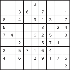
Figure 13.3 shows how to create a new 17-clue puzzle. The generator strips two clues from an 18-clue puzzle, adds a new clue, and then uses the solver to search for any valid solutions.
Figure 13.3 The generator and solver
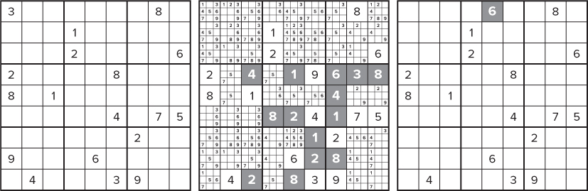
As shown in Figure 13.4, clues 3 and 9 in the left-hand puzzle are first removed from the first column. The generator then populates each unsolved cell with a list of valid options (see the middle puzzle). The gray values are values where the cell can hold only one value. The solver then recursively prunes down the options to find a valid puzzle, taking care that no redundant clues exist (see the right-hand puzzle). The gray number 6 is the new clue that has been added.
Figure 13.4 Creating a 17-clue Sudoku puzzle
This method of creating a new puzzle is known as the minus-two-plus-one algorithm. A similar technique is used to find the “thirty-niner.” Taking an existing “thirty-eighter,” one clue is removed and two new clues are added — in other words, a minus-one-plus-two algorithm.
Optimizing the Solver Using SSE Intrinsics
Modern CPUs have instructions that can work on more than one data item at the same time — that is, Single Instruction Multiple Data (SIMD) instructions. Examples of such instructions include MMX and the various Streaming SIMD Extensions (SSE, SSE2, and so forth). Because these instructions work on more than one element of data at a time, the resulting code is referred to as vectorized code. Vectorization is covered in detail in Chapter 4, “Producing Optimized Code.” Vectorized code runs much faster than code that has not been vectorized.
SSE intrinsics are compiler-generated assembler-coded functions that can be called from C/C++ code and that provide low-level access to SIMD functionality without the need to use an inline assembler. Compared to using an inline assembler, intrinsics can improve code readability, assist instruction scheduling, and help reduce the debugging effort. Intrinsics provide access to instructions that cannot be generated using the standard constructs of the C and C++ languages.
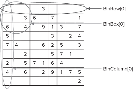
The Intel compiler supports a wide range of architectural extensions, from the early MMX instructions to the latest generation of SSE instructions. By using these SIMD instructions, it is possible to do some quite creative manipulation of the puzzle data. SSE2 (and later) supports 128-bit registers, and the individual bits of these can be used to hold all the data in a Sudoku puzzle. Note that only the first 81 bits need be used to represent all the cells on a Sudoku board. Each bit in the 128-bit array values corresponds to a cell location. The 128-bit value at BinNum[0] records any cell containing a 1. BinNum[1] records any cell that contains a 2, and so on. Figure 13.5 gives an example of how this happens.
Figure 13.5 A typical Sudoku puzzle that stores its numbers into 128-bit variables
The following code shows how the values in Figure 13.5 would be stored in the BinNum array:
_m128i BinNum[9];        // Declare array of 128-bit values

BinNum[0] = 0x400100;     // 1's in cells 9 and 23
BinNum[1] = 0x800000000;  // 2's in cell 36
  .
  .
BinNum[8] = 0x80088000;   // 9's in cells 16, 20 and 32
To find out if a puzzle holds a particular value, predefined masks are used. The masks are again held in an array of 128-bit SSE variables:
_m128i BinBox[9];      // holds binary mask of all boxes
_m128i BinRow[9];      // holds binary mask of all rows
_m128i BinColumn[9];   // holds binary mask of all columns
These masks hold binary bitmaps representing a whole row, column, or box, as shown in Figure 13.6. BinRow[0] represents the first row; BinRow[1] represents the second row; and so on. For example:
BinRow[1] = 0x3FE00;   // mask for row 2
BinBox[0] = 0x1C0E07;  // mask for box 1
Figure 13.6 The rows, columns, and boxes of the Sudoku grid are represented by an array of registers
To check if row 2 contains a 3 now only requires the mask of row 2 to be ANDed with the variable for number 3, as follows:
Result = BinRow[1] & BinNum[2];
The result will be nonzero if row 1 does contain a 3; otherwise, the result will be zero.
The first version of the Sudoku generator did not use SSE instructions or intrinsics. Reworking the first version of the code to use SSE2 registers took a significant amount of time. Using SSE2 registers and adding SSE intrinsics resulted in a speedup of several hundred times using the same hardware.
Using SSE intrinsics does have drawbacks, because it is possible to end up locking your implementation to a particular generation of architecture. Also, the long names of the SSE functions can make your C++ code almost unreadable, and there is a significant learning curve for the programmer to climb. Only experience can determine when it is advantageous to use intrinsics. However, in the case of the Sudoku generator, the performance improvement far outweighed the extra effort required.
If you want to examine the code in more detail, download the code that is used in the hands-on section.
Adding Parallelism to the Generator
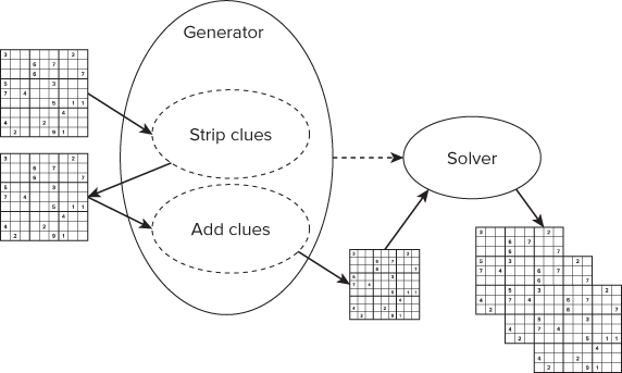
Intel VTune Performance Analyzer was applied to the Sudoku generator, allowing hotspots to be identified within code. The biggest hotspot, which was found to be in the top hierarchy of the generator, was then parallelized using OpenMP tasks.
OpenMP tasks, introduced in OpenMP 3.0, can be used to add parallelism to loops, linked lists, and recursive calls. OpenMP tasks are good at producing balanced loads, especially when the amount of work between each loop may be uneven; the same is true for linked lists and recursive calls.
![]()
Listing 13.1 shows how a number of tasks were created in a single-threaded loop. Each task was then scheduled and run by the OpenMP run time. As a thread completes the execution of one task, it is given another task to execute.
 Listing 13.1: Using OpenMP tasks to add parallelism to the generator
1: int node;
2: #pragma  omp parallel shared(omp_log, node)
3: {
4:   #pragma omp single nowait
5:   {
6:     for(node = 0; node < Num_SudokuNode ; node++)
7:     {
8:       #pragma omp task firstprivate(omp_log, node)
9:       {
10:        int result = AddClues(SudokuNode[node], omp_log);
11:      }
12:    }
13:  }
14: }
code snippet Chapter1313-1.cpp
The code is part of the minus-one-plus-two algorithm. The SudokuNode[] array holds a number of Sudoku puzzles that have already had one clue removed. For example, when looking for a new “thirty-niner,” this array would hold 38 copies of a “thirty-eighter,” with one clue having already been removed sequentially from each puzzle. Each puzzle is then filled with an additional two clues by a call to AddClues(), with the number of successfully generated puzzles being returned. The omp_log variable points to a file that is used to store each new “thirty-niner” that is generated.
At line 2, the OpenMP run time creates a pool of threads (as explained in Chapter 7). By default, the number of threads is the same number as the number of hardware threads the environment can support, although the programmer can override this.
The code between lines 4 and 13 will run on just one thread. The enclosed loop is responsible for creating a number of tasks that will be run in parallel, with each thread running one task at a time. At line 8, an OpenMP task is created on each iteration of the loop. The tasks are free to start execution straight away. Variables outside the parallel region, which is defined by the first pair of braces, are visible to all threads by default. To make a thread have a private instance of such a variable, you use the private or firstprivate keyword. In line 2, the shared keyword is redundant, because the default behavior of OpenMP is that all data is shared. The shared keyword is added here as a reminder to the programmer that the variables omp_log and node can be accessed by all the threads.
Adding firstprivate at line 8 causes the OpenMP run time to create private copies of the variables omp_log and node for each created task. A firstprivate variable differs from a private variable in that a firstprivate variable is automatically initialized with the values from the shared variable, whereas a private variable is uninitialized.
There is an implicit barrier at line 13: the end of the omp single thread. To allow the single thread to be made available to execute some of the newly created OpenMP tasks, the nowait keyword has been added at line 4. Without this keyword, once the single thread had completed creating the OpenMP tasks, it would simply sit at line 13 until all the other threads have completed their execution. By adding nowait, the efficiency of the threaded execution is improved by making the single thread available for joining in executing the tasks.
The Results
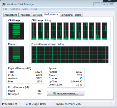
Once the parallel code was added to the project, it was rewarding to see that on a quad-cored machine running hyper-threading, which can support 12 hardware threads, all 12 hardware threads were kept busy. Figure 13.7 shows that with the parallelism implemented in the code, each hardware thread ran at 100 percent. However, it should be emphasized here that the goal is to reduce overall time, not just to increase CPU utilization.
Figure 13.7 A fully utilized CPU
One of the most difficult aspects of adding OpenMP was grasping how variables were treated. Much of the time taken was used in reworking the code so that there was less need to share data between the different running tasks. Some effort was also spent on reducing the number of dependencies between loops so that they could be easily parallelized. Adding the parallelism took about two weeks of work, which felt like a lot of effort at the time, but in relation to the length of the project, the time was fairly short.
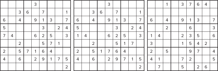
As a result of the work done, three new “thirty-niners” were discovered, as shown in Figure 13.8.
Figure 13.8 The three 39-clue minimal solutions found using the minus-one-plus-two search
Hands-On Example: Optimizing the Sudoku Generator
The code used for this hands-on section shows how to optimize a Sudoku generator by using the same techniques as those used in the project that led to the first “thirty-niner.” The sample code does not check for redundant clues or log the results correctly. Some error checking has also been ignored. This was done to make the example simpler and easier to understand and to reduce the required computation time.
The code consists of a solver and a generator. The solver uses a brute-force recursive algorithm to solve a partially populated puzzle. The generator creates a stack of partially populated puzzles that are passed on to the solver. The algorithm used in the generator is the minus-two-plus-one search.
About the Code
The code for the hands-on activities is available for download as a Visual Studio project (Chapter13sudoku.zip). As you work your way through the activities, you will be asked to switch to different configurations, with names such as STEP_1, STEP_2, and so forth (using the drop-down configuration menu in Visual Studio). As you swap configurations, different preprocessor macros will be automatically added to the build parameters of the project.
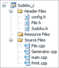
A number of header files are associated with the project. Of particular note is Config.h, which contains macros to control inclusion of different optimization features. The various source files are as follows:
- File.cpp contains fairly rudimentary code that reads a single-line text file containing a partially completed Sudoku puzzle.
- Generator.cpp holds the code for the minus-two-plus-one code.
- Main.cpp holds the main body of the code for the solver.
- Print.cpp contains code to print the clues and puzzles to the screen.
Figure 13.9 gives the project structure as seen within Visual Studio.
Figure 13.9 The code consists of a number of source files and a user-editable Config.h
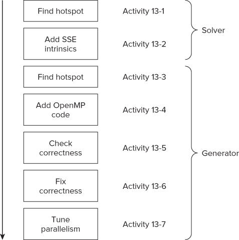
In this hands-on section there is no need to change any code. All the required changes are added automatically when you choose the correct build configuration. Figure 13.10 shows the seven activities in this hands-on section. Activity 13-1 uses the Microsoft compiler, and then switches to the Intel compiler.
Figure 13.10 The solver is first optimized and then parallelism is added to the generator
The reasons for using the Microsoft compiler and then switching to the Intel compiler are as follows:
- The original Sudoku project started with the Microsoft compiler.
- To show that Intel VTune Amplifier XE can be used with the Microsoft compiler. (This is also true of Inspector and Advisor.)
- To show how to swap to the Intel compiler.
- To take advantage of the optimized code that the Intel compiler produces.
- The Intel compiler supports Open MP tasks, which is not currently the case with the Microsoft compiler.
The running program accepts a single-line file as input, where each cell is represented by a digit. Where there is no clue, a zero is placed instead. The test.txt file is used in the hands-on exercise and contains the following:
000704005020010070000080002090006250600070008053200010400090000030060090200407000
![]()
The Solver
Figure 13.11 illustrates the solver's recursive backtracking algorithm.
Figure 13.11 The solver uses a recursive backtracking algorithm to solve the puzzle

The solver first is passed a partially completed puzzle (Table A). For simplicity, only the top-left corner of the puzzle is shown. The solver starts at the first empty cell, Idx1 (row 1, column 2), which could be assigned the values 4, 7, or 9 (determined by the clues in the same row, column, and box). The solver is called recursively two more times, taking the cells Idx2 (row 1, column 3) and Idx 20 (row 3, column 3). The table now looks like Table B. Because Idx 20 cannot legitimately be filled with any value, the solver returns, removing the cell content of the cells along the way. The solver returns back to Idx 1 and places the next available clue (7) and in Idx1 and does a fresh recursive call. The solver then fills the next empty cell (Idx 2) with the lowest potential clue (4). This is followed by another recursive call, in which Idx 20 is filled with the value 9. The puzzle now looks like Table C. This recursive procedure is continued until the puzzle is solved.
Listing 13.2 shows the structures used in the solver. The SUDOKU structure contains an array of 81 NODE structs.
Listing 13.2: Structures used in the solver
1:  typedef struct NODE
2:  {
3:     int cell;
4:     int number;
5:     int TempCellsLeft;
6:  }_NODE;
7:
8:  typedef struct SUDOKU
9:  {
10:    NODE Nodes[NUM_NODES];
11: }_SUDOKU;
code snippet Chapter1313-2.cpp
Listing 13.3 shows the solver's recursive algorithm. When the solver is first called, it is passed pPuzzle, which is a pointer to the current puzzle, and NodeIdx, which is an index to the current cell that is being considered.
Listing 13.3: The solver's recursive code
1: bool Solve(SUDOKU *pPuzzle,int PuzzleIdx,int NodeIdx,int &NumRecursions)
2: {
3:     NumRecursions ++;
4:     if (NodeIdx >= NUM_NODES)
5:         return true;
6:
7:    if(!FillPossibilities(pPuzzle,NodeIdx))
8:        return false;
9:
10:    NODE BackupNode;
11:    for(int i=1; i<=MAX_NUM; i++)
12:    {
13:        if(Allowed(pPuzzle,NodeIdx,i))
14:        {
15:          StoreNumber(pPuzzle,NodeIdx,BackupNode,NumRecursions,i);
16:            int NewIdx = GetNextIdx(pPuzzle, NodeIdx);
17:
18:            if (!Solve(pPuzzle,PuzzleIdx,NewIdx,NumRecursions))
19:                ClearNumber(pPuzzle,NodeIdx,BackupNode,i);
20:        }
21:    }
22:    return false;
23: }
code snippet Chapter1313-3.cpp
In line 7, the solver first populates the partially populated puzzle's empty cells with a list of all valid possibilities. The loop at line 11, which iterates from 1 to 9, along with the call to Allowed, is used to drive the next recursive call to Solve at line 18.
If Solve fails, it returns false; otherwise, it returns true — once it has visited all the nodes in the puzzle (line 8). Each time Solve is called, the NewIdx (line 16) is incremented to point to the next empty cell in the puzzle.
Finding Hotspots in the Solver
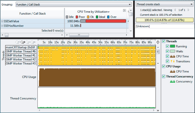
The details of using Intel Parallel Amplifier are presented in Chapter 6, “Where to Parallelize,” and need not be repeated here. However, Activity 13-1 lists the steps for using Amplifier to find the hotspots within the code. As mentioned in Chapter 6, it is good practice to optimize the serial code first, before making any code parallel. Code that consumes significant amounts of the total run time of the program is the ideal candidate for optimization. After running Amplifier, you can see that the biggest consumer of CPU time is the NumInRow function, closely followed by NumInColumn (see Figure 13.12).
Figure 13.12 Intel Parallel Amplifier shows the hotspots in the solver code
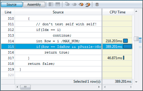
Examining the code of the first hotspot within Parallel Amplifier shows that the majority of the time consumed is due to two things: the iteration of the array of nodes and the divide calculation (see Figure 13.13).
Figure 13.13 The code of the solver hotspot
Optimizing the Code Using SSE Intrinsics
The code in the STEP_2 version of the project has been changed to use SSE intrinsics, as described in the first part of this case study. The following SSEHasNumber function is used for checking the existence of a number in a row column or box:
1: bool SSEHasNumber(SUDOKU *pPuzzle,_m128i BinArray[], int i, int j)
2: {
3:     _m128i Tmp1 = ( _mm_and_si128(pPuzzle->BinNum[j-1], BinArray[i]));
4:     _m128i Tmp2 = _mm_setzero_si128();
5:
6:     Tmp2 = _mm_cmpeq_epi32(Tmp2, Tmp1);
7:
Once the new code is included in the build (by choosing the STEP_2 build configuration in Visual Studio), the total execution reduces significantly, giving a speed up of 12 when using the same hardware as the serial version (see Table 13.1).
Table 13.1 Speedup with and without SSE Intrinsics
| Time (Seconds) | Speedup | |
| Without SSE | 1.78 | 1 |
| With SSE | 0.14 | 12 |
The Generator
The generator uses a minus-two-plus-one search algorithm to remove two clues from an existing puzzle, and then traverses the puzzle, filling in each empty square with a new clue before passing the partially completed puzzle on to the solver.
The code consists of four nested loops:
- The outermost loop removes the first clue and creates a copy of the puzzle.
- The second nested loop is responsible for removing the second clue.
- The third nested loop traverses through each empty cell, using the innermost loop (the fourth loop) to try out all the new potential clues in the current cell.
To summarize, the outermost loop and the second nested loop are responsible for the minus-two part of the search, and the other two loops are responsible for the plus-one part.
Finding the Hotspots in the Generator
When parallelizing a hotspot, the usual rule of thumb is that it is not the hotspot itself that is parallelized, but rather the parallelism is added higher up in the calling sequence. Activity 13-3 shows the steps involved with running Intel Parallel Amplifier on the generator code to reveal hotspots.
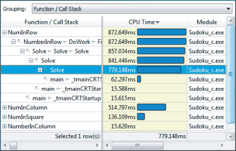
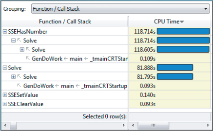
Activity 13-3 reveals that the main hotspot is SSEHasNumber, which is called by Solve, which, in turn, is called by GenDoWork. The GenDoWork function is called from the outermost loop in the generator code. Figure 13.14 shows these relationships.
Figure 13.14 Using Amplifier to find the generator hotspots and calling sequence
Adding Parallelism to the Generator Using OpenMP
After using intrinsics and vectorization (SSE instructions), further enhancements in speed are obtained by adding parallelism. This is accomplished by adding OpenMP tasks to the code high up in the calling hierarchy of the generator. In Listing 13.4, OpenMP-specific code is added to lines 5, 8, and 14. This code works in a similar manner to Listing 13.1.
Listing 13.4: Adding OpenMP tasks to the generator
1: SUDOKU Puzzles[NUM_NODES];
2:
3: int Generate(SUDOKU *pPuzzle)
4: {
5:      #pragma omp parallel
6:      for(int i = 0 ; i < NUM_NODES -1; i++ )
7:      {
8:          #pragma omp single nowait
9:          {
10:             NODE Node1 = pPuzzle->Nodes[i];
11:             if(Node1.number > 0)
12:             {
13:                 memcpy(&Puzzles[i],pPuzzle,sizeof(SUDOKU));
14:                 #pragma omp task firstprivate(i)
15:                 GenDoWork(&Puzzles[i],i);
16:             }
17:         }
18:     }
19:     return gNumCalls; //global incremented on each call to solver
20: }
code snippet Chapter1313-4.cpp
Using the same architecture as the nonparallelized code, the application ran nearly 7 times faster on a machine that had 12 threads (see Table 13.2).
Table 13.2 Speedup with and without OpenMP
| Time (seconds) | Speedup | |
| Without OpenMP | 213 | 1 |
| With OpenMP | 32 | 6.7 |
Checking Correctness in the Generator
It is essential when introducing parallelism into code to check for data races and other similar problems. Activity 13-5 involves running the Intel Parallel Inspector to search for problems that may occur when parallelizing code. The results show several data races that need to be resolved (see Figure 13.15).
Figure 13.15 The Inspector reveals several data races

Fixing Correctness in the Generator
The data races are caused by the following three things:
- Reading/writing the global variable gNumSolutions without appropriate synchronization
- Reading/writing the global variable gNumCalls, again without appropriate synchronization
- Calling the std::map functions
To solve the data races, you need to protect the access to the global variables by adding a synchronization directive. Various OpenMP directives were covered in Chapters 8 and 9. To fix the gNumSolutions and gNumCalls data races, you can use the atomic directive, as follows:
#pragma omp atomic
   gNumSolutions++;

#pragma omp atomic
   gNumCalls++;
To fix the data race caused by calls to std::map functions, wrap the call to StoreSolution within a critical section using the #pragma omp critical directive:
// StoreSolution returns true if solution is unique
#pragma omp critical
{
                   res = StoreSolution(pPuzzle,PuzzleIdx);
}
Tuning Performance
After correcting errors in the parallel code, the next step is to tune the application with respect to parallelism. Typically, you need to address the following issues:
- Parallel overhead
- Load balancing
- Scalability
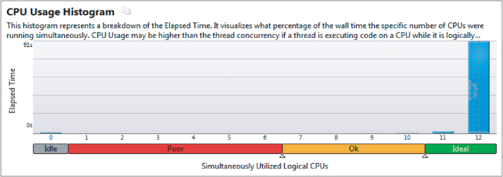
In Activity 13-7, you solve the load-balancing problem using Intel Parallel Amplifier XE (refer to Chapter 9 for more details). Using Amplifier to analyze the code shows the newly parallel code apparently performing well. Amplifier reports that all 12 logical CPUs are fully utilized (see Figure 13.16). The color of the scale indicates how good the concurrency is. The color of the scale indicates how good the concurrency is. In this case, the large histogram block in the Ideal section (colored green on your PC) shows excellent CPU usage.
Figure 13.16 Apparently all the cores are being used, which hides an underlying problem
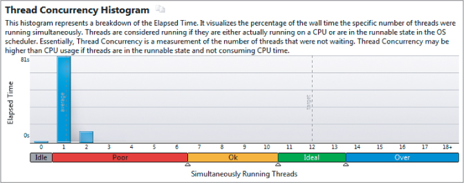
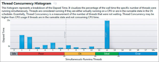
On closer examination, you can see that although the CPU usage is high, the number of simultaneous running threads is poor (see Figure 13.17).
Figure 13.17 The program is running with very poor concurrency
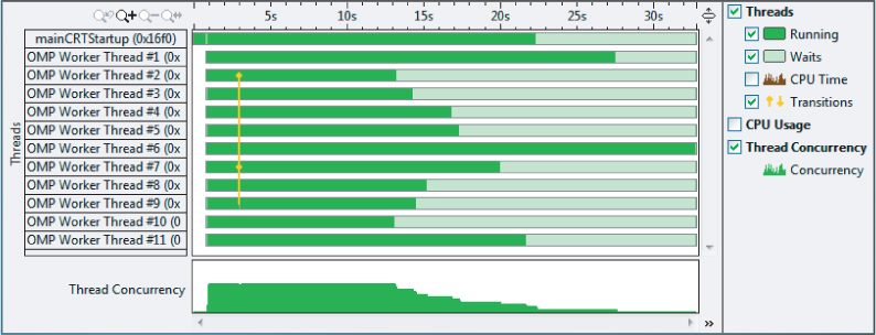
Looking at the time line, you can see a lot of vertical transition lines (see Figure 13.18). A healthy program should not be dominated by these transitions.
Figure 13.18 The timeline is dominated by vertical transition lines
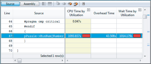
Looking at the source view of the bottleneck, it is clear that an ill-placed #pragma omp critical directive is the cause of the problem (see Figure 13.19).
Figure 13.19 The reason for the poor concurrency is the critical section
Removing the #pragma omp critical directive leads to a better concurrency (see Figure 13.20).
Figure 13.20 Removing the critical section leads to a better concurrency
Even though the program has a reasonable concurrency level, not all threads are doing the same amount of work. As shown in Figure 13.21, some threads finish their work much earlier than others. Although some further work could be carried out to try to improve the balance, the performance is quite adequate.
Figure 13.21 Not all threads are doing an equal amount of work
Summary
The Sudoku puzzle case study gives a fascinating insight into how carefully crafted code using SSE intrinsics can lead to dramatic performance improvements over non-SSE code. Parallelizing using OpenMP tasks can produce well-balanced parallel applications.
The skills used to produce solutions for Sudoku puzzles in this chapter can readily be used in many applications to produce efficient and optimized code.
Chapter 14, “Nine Tips to Parallel-Programming Heaven,” explores an alternative way of parallelizing using Intel Cilk Plus. The techniques learned there can likewise be applied to this Sudoku problem.