Chapter 10

Parallel Advisor–Driven Design

What's in This Chapter?

Using Parallel Advisor

Surveying the application

Adding annotations

Assessing suitability

Checking for correctness

Moving from annotations to parallel implementations

This chapter introduces a parallel development cycle that uses Intel Parallel Advisor. Advisor helps programmers become more productive, because it reveals the potential costs and benefits of parallelism by modeling (simulating) this behavior before programmers actually implement the parallelism in their code.

Using Parallel Advisor

The problem that Advisor helps you solve is to parallelize existing C/C++ programs to obtain parallel speedup. Advisor's value is increased productivity; it enables you to quickly and easily experiment with where to add parallelism so that the resulting program is both correct and demonstrates effective performance improvement. The experiments are performed by modeling the effect of the parallelism, without adding actual parallel constructs.

Advisor is a time-tested methodology for successfully parallelizing code, along with a set of tools to provide information about the program. Advisor has several related personas:

• A design tool that assists you in making good decisions to transform a serial algorithm to use multi-core hardware
• A parallel modeling tool that uses Advisor annotations in the serial code to calculate what might happen if that code were to execute in parallel as specified by the annotations inserted by the user
• A methodology and workflow to educate users on an effective method of using parallel programming

The objective of parallelization is to find the parallel program lurking within your serial program. The parallelism may be hiding due to the serial program being over-constrained — for example, having read-write global variables that cause no problems for serial code but inhibit parallelism.

Advisor is not an automatic parallelization tool. It is aimed at code that is larger and messier than simple loop nests. Instead, it guides you through the set of decisions you must make, and provides data about your program at each step. In summary, Advisor provides a lightweight methodology that allows you to easily experiment with parallelism in different places.

Your parallel experiments with Advisor may all fail, which can be a blessing in disguise — you can avoid wasting time trying to parallelize an inherently serial algorithm. You may need to investigate alternative algorithms that can be parallelized, or just leave your program serial and investigate serial optimizations.

Who can use Advisor?

• Architects — To design where introducing parallelism will provide the best return on investment (ROI): improved performance for a reasonable development cost.
• Developers — To discover opportunities for parallelization and modify the program to make it parallel-ready. A program is parallel-ready when there is a predicted parallel speedup and no predicted data-sharing (correctness) issues exist.

The key technology in Advisor is the use of parallel modeling of the serial program. You don't actually add parallelism to your code — you just indicate where you want to add it and the Advisor tools model how that parallel code would behave. This is a huge advantage over having to immediately add parallel constructs. Your still-serial program doesn't crash or produce incorrect results because of incorrect and likely nondeterministic parallel execution (such as unprotected data sharing among tasks). Test suites generate identical results, because your serial program will not show the nondeterminism caused by parts of the program running in different orders due to parallelism. This also enables you to refactor your program to remove data-sharing errors and make it parallel-ready, while it is still serial.

Advisor does have some disadvantages, compared with plunging ahead and immediately adding parallel constructs:

• You have to add annotations to describe where you want to experiment with parallelism. Later, you convert them to parallel constructs.
• Analyzing (modeling) the correctness of the pretend tasks' use of shared memory can be significantly slower than the program's normal execution time. Not only do you use a Debug build, but the Correctness tool also must instrument and track every load and store as the program runs to detect these kinds of errors. But it has the advantage of relatively quickly finding problems that are otherwise difficult to uncover using traditional debugging techniques.
• The tools analyze your running program, so they tell you only about parts of the program that are actually executed. However, you would encounter this same limitation by attempting to introduce parallelism immediately.

Understanding the Advisor Workflow

Intel Parallel Advisor guides you through a series of steps (see Figure 10.1). In practice, programmers usually move back and forth between some of the steps until they achieve good results.

Figure 10.1 The five-step Advisor workflow

The Advisor Workflow tab guides you through these steps, highlighting the current step in blue (see Figure 10.2). The Start buttons are used to launch each analysis, and the Update buttons are used to re-run an analysis tool. You can view the results by pressing the blue right arrow button.

Figure 10.2 The Advisor Workflow tab

The following five basic steps help you find hidden parallel programs:

Now that you have a parallel program, you can apply the rest of Parallel Studio.

You can follow several strategies for investigating multiple parallel region (site) opportunities:

• Depth-first — Take a region through all steps before picking another region; you can focus on the behavior of one region of code.
• Breadth-first — Take all regions through the steps together; you can focus on the purpose and information provided by each tool.
• Modified depth-first — Take each region through the final correctness checking step, and then convert all regions to parallel constructs together; your program remains serial for as long as possible, preserving the benefit of identical test suite results.

Finding Documentation

Advisor provides copious documentation, which you can access in one of the following ways:

• Help ⇒ Intel Parallel Studio 2011 ⇒ Parallel Studio Help ⇒ Advisor Help
• Help ⇒ Intel Parallel Studio 2011 ⇒ Getting Started ⇒ Advisor Tutorial
• The Workflow tab and its hot links into Advisor help
• Visual Studio context-sensitive F1 help
• Right click in any Advisor report, and choose “What should I do next?”

Getting Started with the NQueens Example Program

This chapter uses the NQueens example program that ships with Advisor to demonstrate how Advisor works. Listing 10.1 shows the two functions, setQueen() and solve(), that are the focus of the analysis.

Listing 10.1: The setQueen() and solve() functions

void setQueen(int queens[], int row, int col)
{
    int i = 0;
    for (i=0; i<row; i++) {
        // vertical attacks
        if (queens[i]==col)
        return;
        // diagonal attacks
        if (abs(queens[i]-col) == (row-i) )
        return;
    }

    // column is ok, set the queen
    queens[row]=col;

    if (row==g_nsize-1)
    {
        nrOfSolutions ++;
    }
    else {
        // try to fill next row
        for (i=0; i<g_nsize; i++)
            setQueen(queens, row+1, i);
    }
}

void solve(int size)
{
    g_nsize = size;

    for(int i=0; i<g_nsize; i++)
    {
        // create separate array for each recursion
        int* pNQ = new int[g_nsize];

        // try all positions in first row
        setQueen(pNQ, 0, i);

        delete pNQ;
    }

}

The NQueens program computes the number of ways you can place n queens on an nxn chessboard with none being attacked. It prints the result and the elapsed time. The program's default value for n is 13. The NQueens algorithm proceeds in the following way. The loop in the solve() function places a queen in each of the size columns of the first row, and then calls the setQueen() function to place queens in the remaining rows. The setQueen() function tries a queen in each column of the next row. If it doesn't “fit,” setQueen() goes to the next column. If more rows exist, it calls itself recursively on the next row; otherwise, a solution has been found and the nrOfSolutions global variable is incremented — and in these cases setQueen() also goes on to the next column.

You can find the nqueens_Advisor.zip file that ships with Advisor in the Samples<locale> folder in the Parallel Studio 2011 install folder, usually C:Program FilesIntelParallel Studio 2011. Unzip the file into a writable folder. Start Visual Studio 2005, 2008, or 2010, and open the solution file nqueens_Advisor queens_Advisor.sln in that folder; for VS 2008 or 2010, the .sln file will be converted — follow the wizard's directions.

Figure 10.3 shows the Advisor toolbar, which appears in the Visual Studio toolbar area. It provides one of the several ways of invoking Advisor and the Advisor tools.

Figure 10.3 The Advisor toolbar

You should start by opening the Workflow tab. In addition to using the toolbar, you can start the three analysis tools from the Workflow tab either by clicking the corresponding button or by selecting VS Tools ⇒ Intel Parallel Advisor 2011.

Surveying the Site

Recall the discussion of Amdahl's Law in Chapter 1, “Parallelism Today,” which says that parallel speedup is limited by the execution time of the portion of the program that remains serial. The obvious conclusion is that you need to discover where your serial program spends the most time and focus there in order to find the most effective parallel speedup.

This is what the Survey tool helps you do: it runs and profiles the program to show where the program spends its time.

Your goal in this step is to find candidate parallel regions. You make the decisions — the Survey tool provides timing information and helps you navigate your program. You may already have candidate regions in mind, but run a Survey analysis anyway so that you have quantitative data about how much time is spent in each portion of the program.

If you were doing serial optimization, you would find hotspots that have the highest Self Time and reduce the time there (that is, by reducing the number of executed instructions). Looking elsewhere will not help serial execution time!

In contrast, with parallel optimization you don't need to focus just on a hotspot — you can also look along the chain of loops and function calls from the application's entry point to the hotspot for candidate parallel regions that have high Total Time — time spent there and in called functions (including the hotspot). This is because the objective of parallel optimization is to distribute the execution time (the executed instructions) over as many tasks/cores as possible. The parallel program typically executes more instructions than the serial program (due to task overhead), but it consumes less elapsed time because the work is spread among multiple tasks at the same time on multiple cores.

Running a Survey Analysis

To run a Survey analysis, begin by building a release configuration of your program. For best results, turn on debug information so that the Survey tool can access symbols, and turn off inlining so that all functions in the source-level call chain appear in the Survey Report. Survey analysis has low overhead — it allows the program to execute at nearly full speed — so employ a data set that exercises the program the way it is normally used. Start the Survey analysis using the Advisor toolbar, Workflow tab, or the Tools ⇒ Intel Parallel Advisor 2011 menu.

The Survey Report

The Survey Report for NQueens has several columns (see Figure 10.4):

• Function Call Sites and Loops — Call/loop chains starting from the main entry point (upper left). All distinct chains appear, sorted by highest Total Time toward the top. You can use the [+] or [–] to open/close a call chain, respectively.
• Total Time % (and Total Time) — The percentage of and actual elapsed time, respectively, spent in a function or loop and all functions called from this location (used to estimate the time that could be covered by a parallel region).
• Self Time — Elapsed time spent in only the function or loop (used to find hotspots).
• Source Location — The file name and line number of the function or loop.

Figure 10.4 The Survey Report for NQueens

Finding Candidate Parallel Regions

The basic strategy is to look along hot call/loop chains in the Function Call Sites and Loops column from the upper left toward the lower right for candidate parallel regions:

• Data parallelism — Loops can be promising parallel regions because if each instance of the loop body can be a task, then you naturally create numerous tasks (one per iteration) over which to distribute the execution. This is why the Survey Report displays loops as well as calls.
• Task parallelism — Alternatively (or in addition on the same call/loop chain as a candidate loop), look for a high Total Time function F that makes direct calls to several functions G and H that also have high Total Times — for example, F: 60%, G: 40%, H: 20%. The calls to G and H could be put in two different tasks that can execute in parallel, assuming G and H are “independent.” This can provide scaling that seems to be limited to 2 cores (but see the following “nested parallelism” bullet).
• Nested parallelism — Several candidate regions along the same call chain; inner parallel regions are “nested” within outer parallel regions. For example:
  • Several directly nested loops. If you select the m outer iterations and the n inner iterations as tasks, there will be m*n parallel tasks executing the body of the inner loop.
  • Task parallelism in a recursive function. For example:

    Qsort(array) {
        Partition array into [less_eq_array, "center" element, greater_array];
        Qsort(less_eq_array);
        Qsort(greater_array);
        }
    

    With task parallelism the two recursive Qsort calls occur in different tasks. At each level of the recursion you get 2, 4, 8, 16, … parallel tasks. So, with this recursive decomposition you are not limited to a fixed number of tasks, even though you see only two tasks in the source code.
• Easy and hard cases — If you can find a candidate parallel region that covers 90 percent of the total time you may be in good shape. In contrast, if you have ten candidates each covering 10 percent of the time, you may have to work harder to get the full parallel speedup.

The Survey Source Window

Double-clicking a loop or function call in the Survey Report takes you to the Survey Source window, which shows the source code to help you determine if this is a good parallel site (see Figure 10.5). The information displayed includes:

• Total Time — Shows the total time spent in a function. Values appear only on some statements.
• Loop Time — Represents the total time over all of the statements in a loop. The value appears on some statement in the loop, often the loop header.
• Call Stack with Loops — Shows the chain of calls used. You can navigate to the source for different locations in the stack by clicking the corresponding stack entry.

Figure 10.5 The Survey Source window

Double-click in the Survey Source window to enter the Visual Studio editor on the corresponding file. Return to the Survey Report from the editor by selecting the My Advisor Results tab for the current Visual Studio project, or click the arrow icon in the “1. Survey Target” section of the Workflow tab. To return from Survey Source to the Survey Report, click the Survey Report button or the arrow icon.

How Survey Analysis Works

When you start a Survey analysis, it runs the current program. Occasionally it takes a sample of where the program is executing, computing the call chain and also noting locations along the chain that are in a loop. When the program completes, the analysis scales the samples to determine the Self Time and the Total Time, sorts the call/loop chains by highest Total Time, and displays the Survey Report. Because the Survey Report employs coarse sampling, there is usually minimal slowdown of the program. The coarse sampling is sufficient because the Survey Report is trying to identify high-frequency events: hotspots and hot call chains.

C:Program Files (x86)IntelParallel Studio 2011Samplesen_US 
queens_Advisor.zip

C:Program FilesIntelParallel Studio 2011Samplesen_US 
queens_Advisor.zip

Annotating Your Code

You communicate to Advisor where you want to try candidate parallel regions by adding annotations to your program. This section describes the parallel model that annotations simulate, the common annotations and parallel constructs they can represent, and how to add them to your program. Recall that Advisor is an inexpensive way to try parallelism in different places. Annotations are cheap — feel free to experiment!

Advisor's Suitability and Correctness tools run your serial program and model how it would behave if it were parallel as specified by the annotations — that is, they pretend it is running in parallel.

Site Annotations

Advisor tools model fork-join parallelism as expressed by the following Advisor annotations:

• ANNOTATE_SITE_BEGIN(<site name>); — After you execute this annotation, subsequently created tasks belong to this site and pretend to run in parallel with other tasks of this site. This is sort of a pretend “fork” point, except tasks are not created until you execute ANNOTATE_TASK_BEGIN.
• ANNOTATE_SITE_END(<same site name>); — Execution of SITE_END is a “join” point for all tasks created in this site; execution pretends to wait here until all owned tasks have completed — that is, the tasks do not run in parallel with code at the same syntactic level following the SITE_END. Note that if the site is (dynamically) nested within another site, tasks of the nested site may run in parallel with other tasks belonging to the parent site.
• ANNOTATE_TASK_BEGIN(<task name>); — Execution of TASK_BEGIN pretends that the code from here to the execution of the matching ANNOTATE_TASK_END(<same task name>); executes in parallel with other “tasks” belonging to the owning site.
• ANNOTATE_TASK_END(<same task name>); — Execution of TASK_END simulates the completion of the execution of the corresponding named task.

Fork-join parallelism is sufficient to model Intel Cilk Plus, OpenMP, and most of the parallel algorithms in Intel Threading Building Blocks (TBB). Following are some examples of Advisor annotations for parallel regions:

• Loop parallelism — To model that the bodies of all iterations of the loop may execute in parallel (also referred to as data parallelism):

ANNOTATE_SITE_BEGIN(big_loop);
     for (i = 0; i < n; i++) {
            ANNOTATE_TASK_BEGIN(loop);
                   Statement1;
                   …
                   Statementk;
            ANNOTATE_TASK_END(loop);
     }
ANNOTATE_SITE_END(big_loop);

• Task parallelism — To model that the two Qsort calls may execute in parallel. Notice that this example also uses recursion:

// Qsort sorts the array a in place, and uses modeled recursive parallelism
void Qsort(array a){
// If a is small enough, sort it directly and return.
// Otherwise, pick an element e from array a.
// Rearrange the elements within a so that it is partitioned in 3 parts
// a == [elements <= e; e; elements > e]
// Let array less_eq_qsort be a reference to the first partition of a
// Let array greater_qsort be a reference to the last partition of a
// Recursively apply Qsort to each of these array references, in parallel.
ANNOTATE_SITE_BEGIN(qsort);
      ANNOTATE_TASK_BEGIN(qsort_low);
              Qsort(less_eq_array);
      ANNOTATE_TASK_END(qsort_low);

      ANNOTATE_TASK_BEGIN(qsort_high);
             Qsort(greater_array);
      ANNOTATE_TASK_END(qsort_high);
ANNOTATE_SITE_END(qsort);
}

• Nested parallelism — This example is an extract from the Tachyon ray tracing example that ships with Advisor:

// Inner loop nest (simplified) from Ray Tracing sample program tachyon_Advisor.
// Two nested loops on y and x, each inner iteration renders
// one pixel in a rectangular grid.
// Processing one pixel is independent of every other pixel, so they
// can all be done in parallel. This is modeled using nested parallelism.
ANNOTATE_SITE_BEGIN(allRows);
    for (int y = starty; y < stopy; y++){
      ANNOTATE_TASK_BEGIN(eachRow);

           ANNOTATE_SITE_BEGIN(allColumns);
               for (int x = startx; x < stopx; x++) {
                   ANNOTATE_TASK_BEGIN(eachColumn);
                      color_t c = render_one_pixel (x, y, …);
                      put_pixel(c);
               ANNOTATE_TASK_END(eachColumn);
               }
            ANNOTATE_SITE_END(allColumns);

        ANNOTATE_TASK_END(eachRow);
    }
ANNOTATE_SITE_END(allRows);

Lock Annotations

Lock annotations can be used to pretend to protect access to shared data by multiple tasks. Note that you usually add lock annotations only after you have run the Correctness tool and have found cases of unprotected data sharing that need to be fixed.

• ANNOTATE_LOCK_ACQUIRE(<address>); — After a task executes this annotation, modeling pretends that no other task may enter a region protected by LOCK_ACQUIRE of the same address — that is, only one task at a time can execute any protected region.
• ANNOTATE_LOCK_RELEASE(<address>); — Execution of this annotation ends the locked region corresponding to <address> — that is, modeling can pretend that another “waiting” task can enter the protected region.

The following example shows how to protect the incrementing of a shared variable inside a task using lock annotations:

ANNOTATE_LOCK_ACQUIRE(0);  // zero is a convenient address
      shared_variable ++;
ANNOTATE_LOCK_RELEASE(0);

Although the preceding examples show paired site and task annotations that match statically in the source code, the paired annotations actually must match at execution time, because they have their parallel modeling effect at run time. So, if multiple execution paths are exiting such a region, it is necessary to have multiple “closing” annotations (two lock-releases in this case):

static int my_lock;
ANNOTATE_LOCK_ACQUIRE(&my_lock);
if (shared_variable == 0) {
             ANNOTATE_LOCK_RELEASE(&my_lock);
             return; }
shared_variable ++;
ANNOTATE_LOCK_RELEASE(&my_lock);

Some other special-purpose annotations are explained in the Advisor documentation.

Adding Annotations

Advisor has some features to simplify adding annotations to your code in the editor. Note that you make the decisions about parallel regions; Advisor helps you generate the correct syntax. To add annotations, follow these steps:

Figure 10.6 The Annotation menu in the editor

Figure 10.7 The Annotation Wizard window

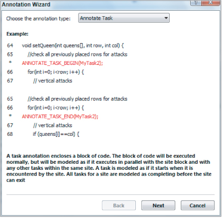
Recall that if the flow of control can leave a region by different paths (for example, a return), it may be necessary to have multiple ending annotations. The Annotation Wizard does not handle this case, so you will need to recognize this situation and insert the additional *END annotation by hand.

Annotations are actually C/C++ macros that expand into calls to null functions with special names; the Advisor tools recognize the names and model the corresponding behavior. And because annotations are just macros, you can employ any C/C++ compiler to build your annotated program.

Every source file using annotations needs to include the file advisor-annotate.h, which defines the annotation macros:

#include "advisor-annotate.h"

The Annotation Wizard in the editor can help with this step. This include file is located in the directory $(ADVISOR_2011_DIR)/include, so you also need to add this include path to the Additional Include Directories in Build Configurations under Properties ⇒ C/C++ ⇒ General for all projects and configurations using annotations.

Checking Suitability

Suitability analysis provides coarse-grained speedup estimates for the annotated code. The purpose of the performance information is to guide your decisions about these sites:

• If the estimate is good, keep going with this site.
• If the estimate is bad, either adjust the site or abandon the experiment.

In either case, you have made progress with a small expenditure of effort because you are using modeling.

You can answer other questions. Does the performance match your expectations from the Survey Report? Are there parallelization-related performance issues (for example, overhead items)?

If you have fixed correctness issues by adding locks or restructuring the code (on the previous iteration through the Advisor workflow), the projected parallel performance may have changed since the last time you ran the Suitability analysis. So, you need to run it again after modifying your annotations or your code.

Running a Suitability Analysis

To run a Suitability analysis, begin by building a release configuration of your program (similar to a Survey analysis, but the program now has annotations) and use the same data set. Start the Suitability analysis from the Advisor toolbar, Workflow tab, or from the Tools menu. The Suitability tool runs the program, analyzing what its performance characteristics might be. There is typically less than a 10 percent slowdown compared to normal program execution. However, if many task instances have a small number of executed instructions, the modeling overhead could be higher and the accuracy of the estimates may suffer. For example, if the average time for tasks is less than 0.0001 seconds (displayed in the Selected Site pane), the instrumentation overhead in the Suitability tool may cause the predicted speedups to be too small.

The Suitability Report

The Suitability Report for NQueens appears in Figure 10.8. It displays the following panes of information. All performance data consists of modeled estimates about how the program might behave if it were parallel.

• All Sites — Summarizes performance information about parallel sites and the whole program and contains:
  • Maximum Program Gain For All Sites — The speedup of the whole program due to all sites, for the current Target CPU Number.
  • A list of each site with their individual Maximum Site Gain (speedup), contribution to Maximum Total Gain of the program, Average Instance Time, and Total Time.
  • Model parameters — Drop-down lists for changing the Target CPU Number and Threading Model. You can select different values to see how the results behave.
• Selected Site — Shows details about the currently selected site in the All Sites pane. The information includes:
  • Scalability of Maximum Site Gain graph — A log-log graph of the site's maximum gain versus the number of CPUs. Each vertical bar shows the range of values for that number of cores, and the ball on the bar shows the estimate with the current set of model parameters and parallel choices.
    • Green area — Good speedup (linear, or close to linear scaling)!
    • Yellow area — Some speedup but there may be opportunities for improvement.
    • Red area — No (or negative) speedup; may need significant effort to improve, or perhaps this site should be abandoned.
  • A list of tasks and locks associated with the current site along with performance information such as maximum, average, and minimum times.
  • Changes I will make to this site to improve performance — Lists five parallel choices you make about sites, tasks, and locks. This area of the pane indicates if any of these items impact performance, and if so, Advisor may recommend how to reduce the impact and what speedup might be achieved. You can change a choice by clicking in the corresponding box. (Click the underlined name for additional documentation.)
    • Reduce Site Overhead — The time to create and complete a parallel site.
    • Reduce Task Overhead — The time to start and stop a task.
    • Reduce Lock Overhead — The time to acquire and release a lock.
    • Reduce Lock Contention — The time spent in one task waiting for another task to release a lock.
    • Enable Task Chunking — Combining multiple tasks into a single task to reduce the task overhead (for example, in a parallelized loop, performing numerous consecutive iterations in one task). Several parallel frameworks, such as Intel Cilk Plus, Intel TBB, and OpenMP, perform task chunking by default.

Figure 10.8 The Suitability Report for NQueens

Double-clicking a site or task name displays the corresponding source code in the Suitability Source window. Return to the Suitability Report by clicking the Suitability Report.

A summary of all your annotations is provided in the Summary Report. This is described in the later section “Replacing Annotations.” An example appears in Figure 10.13.

Parallel Choices

This section describes the meaning and effect of the parallel choice boxes in the Selected Site pane of the Suitability Report.

Figure 10.9 shows the Selected Site pane for a program with lock annotations. In the scalability graph, the balls indicating current estimated gain are in the red, meaning no speedup. However, the bars reach into the green and indicate that there is a range of performance depending on the parallel choices listed to the right. In particular, Advisor shows that a 5.35x speedup can be achieved if you select Reduce Lock Contention, and also recommends that you do so.

Figure 10.9 The Selected Site pane before making a parallel choice

Figure 10.10 shows the result of clicking the Reduce Lock Contention box. The balls in the graph are now in the green, representing very good speedup. By clicking the box, you have agreed to take some action(s) to reduce lock contention when you convert to actual parallel constructs. Note that Advisor only predicts the effect of reducing lock contention — you have the responsibility of implementing that decision later when you add parallel code!

Figure 10.10 The Selected Site pane after making a parallel choice

Using the Suitability Report

You have multiple ways to use the Suitability Report to determine what parallel performance your program might have, and what you might change to achieve improvements. First look at the Maximum Program Gain, and then for each site examine the scalability graph and the parallel choices. Is the program gain what you expected? Change the number of CPUs to check the scalability or to match the number of CPUs on your target platform. Answer the same questions about the gain for each site, and study the scalability graph for each site.

If a site's speedup is low, click it and examine its Selected Site pane:

• In which region of the scalability graph (green, yellow, red) is the result?
• Are there recommended changes to the parallel implementation choices? If so, try clicking the corresponding box.
• How many task instances are there for each site instance? Too few may limit scalability.
• If there are numerous tasks with very small average time, you probably already have recommendations to Reduce Task Overhead and/or to Enable Task Chunking. Task times less than 0.0001 second can cause the instrumentation overhead of the Suitability tool to degrade the accuracy of the speedup estimates.
• Compare Total Time for the tasks with that of the site. Recall that if the tasks cover only 50 percent of the site's time, then Amdahl's Law says the speedup limit is 2x.
• If you have a small number of tasks and a large time deviation, there may be a problem with load balancing (see Chapter 9, “Tuning Parallel Applications”). The large tasks continue running while some tasks finish early and there are no other tasks to run, so some CPUs will be idle. Try to make the amount of work in each task similar, or at least cause the large tasks to start executing first.
• Is the number of locking instances large? This will probably also show up in Reduce Lock Overhead.
• Is the Total Time in locks similar to that for tasks? This may also show up as a Reduce Lock Contention recommendation.

You can also experiment with the sensitivity of the performance by varying the model parameters and the parallel choices, looking for significant changes in the results. This Sensitivity analysis is fast because all the results have been precomputed — Suitability analysis is not run again.

How Suitability Analysis Works

When you start a Suitability analysis, it runs the current program, keeping track of site, task, and lock annotations, and the time spent in each. It then models what the performance of the program would be if it were run in parallel as specified by the annotations, and for all combinations of modeling parameters and parallel choices. It then displays the coarse-grained estimates in the Suitability Report.

Here is a more detailed description of the Suitability analysis:

• Data collection — While the program runs, the Suitability tool collects timestamps for the beginning and end of each site, task, and lock region, and computes the elapsed times. (Recall that annotation macros expand into calls to specially named null functions; the tool identifies the kind of annotation by the name of the function.) Data collection generates a program trace as a stream of ordered times and information about the regions. It also compresses the data. For example, if 100 consecutive instances of task(foo) are similar, each with about the same elapsed time of 3 seconds, then this could be represented as “100 * task(foo) total 300 seconds.”
• Construct task execution tree — The next step is to build an ordered tree representing the sites and their contained tasks (and nested sites and their tasks) from the ordered stream coming from data collection. Under each tree node for a task are also the instances of locked regions that were executed in the task. The ordering in the tree represents the serial execution order of the regions. To keep the amount of memory consumed by the tree reasonable, the tree is limited to a fixed number of nodes. This is accomplished by employing another kind of compression: if the size limit is reached and more data is still arriving, the tree-building process aggregates the effects of the leaves of a node into the node, and then deletes the leaves. For example, the times for the tasks belonging to a site can be summed and stored in the site's tree node before the tasks' nodes are removed.
• Modeling — The purpose of creating the tree is to provide a structure for modeling the performance characteristics of parallel executions of the program as represented by the annotations. The modeling is performed by simulating the execution of the program in parallel on a fixed number of simulated cores, where the only operations simulated are the beginnings and ends of sites and tasks, and the acquiring and releasing of locks. Time is estimated by using simulated clocks for each core. When a task “runs” on a core, the core's clock is incremented by the time the task took during the data collection run (as stored in the tree).

A key component of parallel modeling is the task scheduler. It has a queue of tasks that are ready to “execute.” The scheduler assigns tasks to cores as the cores complete other tasks. The simulator keeps track of the simulated elapsed time for the sites, tasks, and locks. Note that the simulation does not take into account cache or memory effects from tasks running on different cores. The only inter-task performance impacts are from locks.

The simulation is run for every combination of number of CPUs, threading model, and the five parallel choices, and then the results are saved. When you change one of the values in the Suitability Report, the new result is displayed immediately because it has been precomputed. The reason for building the execution tree is that it is used multiple times for the simulations.

The Target CPU Number affects how many cores are available for the scheduler to allocate to tasks. The Threading Model affects the overheads of individual site, task, and lock operations. The parallel choices have different impacts. For example, the option “fix task overhead” is modeled by having the simulator use zero for task overhead. For the option “fix lock contention,” the simulator never makes a task wait for a lock. (Normally, the simulator causes a task to wait for the lock to be free and records the additional simulated elapsed time for that task.)

Checking for Correctness

You have run the Suitability analysis and are feeling good because you have found some sites that are projected to provide parallel speedups. Now it's time for a reality check; if you parallelize your program in these locations, will there be data-sharing problems or deadlocks that will cause the parallel program to be incorrect? The purpose of checking correctness is to predict if these issues will occur.

Not only does correctness modeling tell you if errors exist, but it also helps you navigate to all of the source locations participating in a data-sharing error or a deadlock. You need this in order to fix the problem.

Or, you may decide that the correctness errors are too difficult to fix or will take too much development time relative to the projected speedup for a parallel site. So, if the return on investment (ROI) is too small, abandon this site and remove its annotations. You have been able to quickly experiment with this site, and now you can go on to other sites.

Running a Correctness Analysis

To run a Correctness analysis, begin by building a debug configuration on your program, making sure that the build configuration uses the dynamic runtime library (Configuration Properties ⇒ C/C++ ⇒ Code Generation ⇒ Runtime Library is /MD or /MDd). Correctness needs optimization off so that all memory references are retained in the generated code, and retained in their original program order, because the modeling tracks all the loads and stores. Correctness modeling causes a significant slowdown of the program, such as 100 times slower. Thus, you should use a reduced input data set to minimize the run time. However, the reduced data set should cause the program to traverse all the paths within the sites. For example, if the Survey or Suitability input data set causes a “parallel” loop to execute one million iterations, it is probably sufficient for correctness modeling if the reduced data set causes the loop to execute only a few iterations. Start the Correctness analysis using the Advisor toolbar, Workflow tab, or Tools ⇒ Intel Parallel Advisor 2011 menu.

As mentioned, performing a Correctness analysis can cause a significant expansion of execution time. So when the Correctness tool is running your program, it displays each “observation” as the program runs. If enough error observations have occurred, you can stop the program by clicking the red Stop button on the Advisor toolbar, or by closing your program's window. A Correctness Report will be created for these observations, even though the program has not run to completion.

The Correctness Report

The Correctness Report for NQueens displays several panes of information (see Figure 10.11):

• Problems and Messages — Correctness combines multiple “observations” into a single “problem”; for example, if an error occurs on the currently indexed element of an array on every iteration of a one-million-iteration loop, you will see one problem instead of having to sift through a million observations on the individual elements of the array.
• Memory reuse: Observations — For the currently selected problem (for example, P1 in Figure 10.11), this section displays a highlighted source line and a surrounding source code “snippet” for the distinct observations (for example, X4, X5) associated with the problem. Clicking the [–] for an observation eliminates the source code lines and shrinks it to a single line describing the observation; clicking the [+] redisplays the source snippet.
• Filter — Lists a number of problems and messages by different categories. Click a line to display only problems and messages in the upper-left pane satisfying that filter category. For example, you can display only problems in a particular file, or only errors (omitting warnings and remarks).

Figure 10.11 The Correctness Report for NQueens

The Correctness Source Window

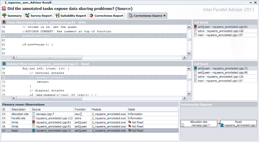
You can navigate to the Correctness Source window by double-clicking the corresponding line in the Correctness Report. Figure 10.12 shows the Correctness Source window for the P1 memory reuse. The following panes of information appear:

• Source code snippets for two observations for the problem (upper-left panes) — Shows more lines of code than in the Correctness Report window. Double-clicking a line navigates to the VS editor.
• Call Stacks for the two source snippets (upper-right panes) — Shows the call stack to get to the displayed source observation. Clicking a function in the stack displays the corresponding source code for that level in the stack.
• Memory reuse: Observations (lower-left pane) — Shows one line for each of the observations for the problem. Double-clicking an observation opens the corresponding source view in the upper pane.
• Relationship Diagram (lower-right pane) — Shows dependencies among the critical observations of the problem. This identifies the important observations and how they relate to each other, which can help you understand the problem.

Figure 10.12 The Correctness Source window for NQueens

Double-click a snippet in the Correctness Source window to enter the Visual Studio editor on the corresponding file. Return to the Correctness Report from the editor by selecting the My Advisor Results tab for the current VS project, or click the arrow in the “4. Check Correctness” section of the Workflow tab. To return from the Correctness Source window to the Correctness Report, click either the Correctness Report button or the arrow.

Understanding Common Problems

Correctness analysis discovers the following four problem categories that you need to understand and fix (or abandon the site). The components of the Correctness Report attempt to assist you in deciphering the cause of the problem.

• Memory reuse — A shared object is referenced by multiple tasks, and in the serial program some tasks that write to the object do so before reading from it. Because multiple tasks are reading and writing the object, this would cause data-sharing problems if the program were actually parallel. However, no values flow from one task to another — they are just “reusing” the same memory. This is called incidental sharing. The tasks are sharing an object but do not need the sharing; instead, each task could use its own copy of the object. Privatizing — providing a private object for each task — is exactly the way to fix this problem.
  Refer to problem P1 in Figure 10.11, which is an instance of memory reuse. The following program fragment shows another instance, where the temp variable declared outside of the parallel site is used to temporarily hold the value of an array element:

static int temp;
…
ANNOTATE_SITE_BEGIN(big_loop);
    for (i = 0; i < n; i++) {
        ANNOTATE_TASK_BEGIN(loop);
            temp = a[i];
            b[i] = … temp …;
        ANNOTATE_TASK_END(loop);
    }
ANNOTATE_SITE_END(big_loop);

ANNOTATE_SITE_BEGIN(big_loop);
    for (i = 0; i < n; i++) {
        ANNOTATE_TASK_BEGIN(loop);
            int temp;
            temp = a[i];
            b[i] = … temp …;
        ANNOTATE_TASK_END(loop);
    }
ANNOTATE_SITE_END(big_loop);

• Data communication — A shared object is referenced by multiple tasks, at least one of which performs a write. In the serial program, values flow from a write in one task to a read in another. This is another instance of a data-sharing problem, but it may be more difficult to resolve than memory reuse. In solving this kind of problem you have to work out whether the data values are independent of each other:
  • Independent updates — This is a case where the tasks are updating an object and the final result does not depend on the order in which the tasks update the object. For example, each task is adding a value to a counter; it does not matter in what order the updates are done, as long as multiple tasks do not access the object at the same time. You can solve this problem by using a lock, which will enforce that only one task at a time is allowed to update the object.
    Problem P2 in Figure 10.10 is a data communication error, which is actually a case of independent updates of the nrOfSolutions variable. (You will investigate and fix this error in Activity 10-4.) Another instance is shown in the following program fragment, which shows a counter that every task (iteration) increments:

    static int counter = 0;
    …
    ANNOTATE_SITE_BEGIN(big_loop);
        for (i = 0; i < n; i++) {
            ANNOTATE_TASK_BEGIN(loop);
                …
                counter++ ;
                …
            ANNOTATE_TASK_END(loop);
        }
    ANNOTATE_SITE_END(big_loop);
    

    It does not matter in what order the increments occur — they just must occur one at a time. The following fragment shows the corrected example with lock annotations added:

    static int counter = 0;
    static int my_lock;
    …
    ANNOTATE_SITE_BEGIN(big_loop);
        for (i = 0; i < n; i++) {
            ANNOTATE_TASK_BEGIN(loop);
                …
                ANNOTATE_LOCK_ACQUIRE(&my_lock);
                    counter++ ;
                ANNOTATE_LOCK_RELEASE(&my_lock);
                …
            ANNOTATE_TASK_END(loop);
        }
    ANNOTATE_SITE_END(big_loop);
    

  • True dependence — If the serial order of access to the object must be retained so that the correct answer is achieved, then the problem is more difficult to fix. It may be necessary to move task boundaries or to combine multiple tasks into a single task (for example, so that multiple references are in a single task), or it may be necessary to abandon this site altogether.
• Inconsistent lock use — A shared object is protected by one lock at one location in the code and by a different lock (or is unprotected) when referenced at another location in the code. Your goal is to protect the object from a data communication error since a lock is used in at least one place. However, because the same lock is not used every time, there might still be a sharing problem. The usual fix is to consistently employ the same lock at all points of reference. The following example demonstrates inconsistent lock use:

  ANNOTATE_LOCK_ACQUIRE(&lock1);
      counter++;
  ANNOTATE_LOCK_RELEASE(&lock1);
  …
  ANNOTATE_LOCK_ACQUIRE(&lock2);
       // protected by different lock
       counter++;
  ANNOTATE_LOCK_RELEASE(&lock2);
  …
  // not protected by any lock
  counter++;
  

  In the preceding code, the counter variable is inconsistently protected by lock1 in the first use, by lock2 in the second use, and is unprotected in the third use.
  Lock hierarchy violations — This is a case where two tasks have nested locked regions, and the locks are acquired in different orders in the two regions. This can cause a deadlock, as described in Chapter 8, “Checking for Errors.” The following example demonstrates a lock hierarchy violation:

  //Region 1
  ANNOTATE_LOCK_ACQUIRE(&lock1);
       ANNOTATE_LOCK_ACQUIRE(&lock2);
       …
       ANNOTATE_LOCK_RELEASE(&lock2);
  ANNOTATE_LOCK_RELEASE(&lock1);
  …
  //Region 2
  ANNOTATE_LOCK_ACQUIRE(&lock2);
        ANNOTATE_LOCK_ACQUIRE(&lock1);
        …
        ANNOTATE_LOCK_RELEASE(&lock1);
  ANNOTATE_LOCK_RELEASE(&lock2);
  

  Imagine that two tasks execute the code snippet above. Suppose that task 1 is about to execute Region 1, and task 2 is about to execute Region 2 at the same time. Task 1 acquires lock1 and task 2 acquires lock2. In order for task 1 to acquire lock2, it has to wait for task 2 to complete Region 2 and release lock2. But in order for task 2 to acquire lock1, it has to wait for task 1 to complete Region 1 and release lock1. Both tasks will wait forever — this is a deadlock.
  The fix is to have all tasks that acquire multiple locks acquire them in the identical order. In other words, they must use the same hierarchy of locks.

Using the Correctness Report

There are several approaches to using the Correctness Report and Correctness Source window to find, understand, and fix sharing problems that would occur if your program were parallel.

Diagnose in detail what is causing each problem by exploring the corresponding source locations and call stacks. The problem statement and observation code snippets in the Correctness Report may be sufficient for discovering the error. For example, if you are incrementing a global counter, you need a lock.

In other cases, the Correctness Source window provides more details about what leads to the occurrence of the problem. One complication is that you have to comprehend the distinct code that two tasks might be executing at the same time, which can cause the interference. Another is that the object being shared might be a parameter, so it may have different names in the two tasks. This is where the call stack is handy; it enables you to examine the source code at different levels of the stack so that you can track how an object is passed through multiple function calls.

Decide if there are too many hard problems to fix for this site, in which case you can either change the location of the site and tasks or abandon the site altogether. Otherwise, fix the problems by employing your understanding of each problem, picking a strategy to fix it, and using the source locations to enter the editor at the appropriate places to make the required source changes.

Rebuild the modified program and run a fresh Correctness analysis to verify that your changes do in fact fix the identified problems and do not introduce new problems. (And after converting your program to parallel constructs, use Intel Parallel Inspector XE to determine if any other classes of memory-sharing problems exist.) Now return to the Suitability analysis step to see what impact these changes may have on performance.

Correctness Analysis Limitation

There is a case of a potential data-sharing problem that Correctness analysis cannot distinguish from the safe usage of a local variable. The potential error is not reported because it would also report errors on the safe case, thus causing false positives. This is one reason you should always run Intel Parallel Inspector XE after adding parallel constructs — Inspector can distinguish these two cases.

The following code fragment demonstrates both a data-sharing issue and a safe usage:

void foo(…) {
    int relatively_global = 0;
    …
    ANNOTATE_SITE_BEGIN(big_loop);
        for (i = 0; i < n; i++) {
            ANNOTATE_TASK_BEGIN(loop);
                int relatively_local = 0;
                …
                relatively_local++ ;  //safe
                relatively_global++ ; //unprotected sharing!
                …
            ANNOTATE_TASK_END(loop);
        }
    ANNOTATE_SITE_END(big_loop);

The relatively_global variable is local to the foo function but global relative to the tasks in the loop. All the tasks share the object, so when it is incremented in the tasks in the parallel program, there is a data-communication error. In contrast, the relatively_local variable is declared within the tasks, and when the program is parallel, each task will have its own copy. So, incrementing relatively_local will not cause a sharing problem.

The issue is that in the serial program, the compiler creates both variables as local stack variables of the foo function. Therefore, the Correctness tool cannot distinguish the two different cases. The design choice was to report either both as errors or neither as errors. The decision was made to avoid annoying false positives and rely on Inspector to catch any true sharing errors. Note that this situation arises only when the task is in a function and the variable declaration (for example, relatively_global) occurs in the same function or the calling function.

How Correctness Analysis Works

When you start a Correctness analysis, it runs the current program, tracking all memory references and annotations that occur. It models which references to the same object could occur in different tasks at the same time if the program were run in parallel, taking into consideration the constraints of which tasks can run at the same time, and lock regions. It then combines related observations into problems and displays them in the Correctness Report.

Here is a more detailed description of Correctness analysis:

• Data collection — While the program runs, Correctness data collection captures the loads and stores them for every object, and also tracks the start and end of each site, task, and lock region.
• Construct task execution tree — The Correctness tool builds an ordered tree representing the sites and their contained tasks (and nested sites and their tasks). The tree is used to answer the question: if two tasks reference the same object, can they be executing at the same time in a parallel program? This is one condition necessary for a data-sharing issue to occur. For efficiency, the tree is constructed and destroyed on-the-fly. For example, if a parallel site is not nested in any other sites, when it finishes executing, it and its tasks can be removed from the tree because they will never be able to execute in parallel with subsequent tasks. So, the answer to the question will be no if one of the tasks is not in the tree.
• Locksets — The set of locks (lockset) that is held by a task at an instant of execution is all the locks that have been acquired without yet being released. If two tasks reference the same object, the tasks can execute in parallel (answer from the tree), and one of the references is a write, then there may be a data-sharing error. If at the time of the two references the tasks hold a lock in common (lockset(task1) & lockset(task2) != NULL), then that lock will prevent them from executing the references at the same instant — thus, no error. However, if the intersection of the locksets is NULL (that is, the locksets are disjoint), a data-sharing problem could occur in a parallel execution.
• Modeling — As the serial program runs, for each load or store, the Correctness tool stores the following information into the model's database associated with the object's address:
• The object's address and size
• Whether it is a read or write
• The current task identity
• The task's lockset

• Can execute at the same time as the current task.
• Has a disjoint lockset.
• Has at least one reference that is a write.

• Correctness Report — Correctness Report processing combines similar observations into single problems that are displayed. For example, there may be multiple observations with different object addresses and task instances, but the referencing instructions have the same line number. This is probably a case of a “parallel” loop iterating through a data structure — you want this reported as only a single problem to be fixed.
• References — The first paper describes the Intel Thread Checker, a tool similar to Advisor's Correctness analysis that models parallelism while executing a serial program. It uses the compiler to insert instrumentation code, whereas Correctness instruments the program as it runs. The second paper describes the use of locksets for finding race conditions.
  • P. Petersen and S. Shah. OpenMP Support in the Intel Thread Checker. Proceedings of WOMPAT 2003, LNCS Springer Lecture Notes in Computer Science, 2716:1–12, 2003.
  • S. Savage, M. Burrows, G. Nelson, P. Sobalvarro, and T. Anderson. Eraser: A Dynamic Race Detector for Multithreaded Programs. ACM Transactions on Computer Systems (TOCS), 15(4): 391–411, November 1997.

Replacing Annotations

When you have a site or sites with good predicted performance and the correctness issues have been resolved, you can convert your parallel-ready program to a true parallel program. First, choose a parallel programming model, such as one of the Intel Parallel Building Blocks, or some other approach. (See Chapter 7, “Implementing Parallelism,” for descriptions of parallel models and how to use them.) Then replace each Advisor annotation with the corresponding parallel construct. This section shows some of these mappings; Advisor documentation contains a more complete set of mappings for Intel Threading Building Blocks and Intel Cilk Plus.

The Summary Report

Figure 10.13 shows the Summary Report, which you can display either by clicking the Summary button at the top of the Advisor window or by clicking the arrow icon for the “5. Add Parallel Framework” step in the Workflow tab.

Figure 10.13 The Summary Report for NQueens

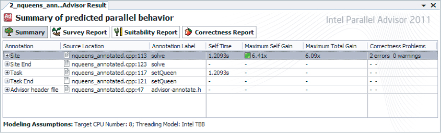
The Summary Report provides a high-level overview of the progress on sites, suitability, and correctness in the program. It shows the kind and location of every annotation in the program. For each site, the report displays the estimated speedup of the site and the entire program (if Suitability analysis has been run) and the number of correctness problems (if Correctness analysis has been run). Figure 10.13 shows the Summary Report for NQueens before the data-sharing problems have been fixed (there are still two errors). The bottom of the report shows the modeling assumptions used (for example, eight CPUs), which you compare against the speedups.

An ROI comparison can be performed from the Summary Report. For a program with numerous parallel sites, you can use the Summary Report to balance the amount of speedup against the amount of development work needed to fix the correctness problems for a site, and then compare the sites to each other to prioritize sites where you can expect the best ROI.

The Summary Report is also the natural place to start when you are moving to parallel constructs, because all the annotations in the program are listed here. Navigate to each annotation so that it can be replaced by a parallel construct, double-click a line for an annotation in the Summary Report to take you into the Visual Studio editor on the file at the line containing that annotation, and then insert the corresponding parallel construct.

Common Mappings

This section shows simple mappings from annotations representing loop parallelism and task parallelism to Intel Threading Building Blocks (Intel TBB) and Intel Cilk Plus. It also demonstrates how to replace lock annotations with the Intel TBB spin_mutex for both Intel TBB and Intel Cilk Plus.

• Loop parallelism

  ANNOTATE_SITE_BEGIN(big_loop);
      for (i = 0; i < n; i++) {
          ANNOTATE_TASK_BEGIN(loop);
              Statement;
          ANNOTATE_TASK_END(loop);
      }
  ANNOTATE_SITE_END(big_loop);
  

  • Intel TBB (using lambda expression)

    #include <tbb/tbb.h>
    …
    tbb::parallel_for(0, n,
        [&](int i) {statement;}
    );
    

  • Intel Cilk Plus

    #include <cilk/cilk.h>
    …
    cilk_for (i = 0; i < n; i++) {
        Statement;
    }
    

• Task parallelism

  ANNOTATE_SITE_BEGIN(qsort);
      ANNOTATE_TASK_BEGIN(qsort_low);
          Qsort(less_eq_array);
      ANNOTATE_TASK_END(qsort_low);
  
      ANNOTATE_TASK_BEGIN(qsort_high);
          Qsort(greater_array);
      ANNOTATE_TASK_END(qsort_high);
  ANNOTATE_SITE_END(qsort);
  

  • Intel TBB (using lambda expressions)

    #include <tbb/tbb.h>
    …
    tbb::parallel_invoke(
        [&] { Qsort(less_eq_array);},
        [&] { Qsort(greater_array);}
    );
    

  • Intel Cilk Plus

    #include <cilk/cilk.h>
    …
    // version 1 for function calls
    cilk_spawn Qsort(less_eq_array);
    Qsort(greater_array);
    cilk_sync;
    
    // version 2 for general statements wrapped in lambda expressions
    cilk_spawn [&] {statement-1}();
    statement-2
    cilk_sync;
    

  The first version is simple because the two statements are function calls. Note that cilk_spawn is not needed on the last task before the cilk_sync. The second version assumes arbitrary statements, so lambda expressions are used to create functions for all but the last statement.
• Locks for Intel TBB and Intel Cilk Plus

  static int my_lock;
  …
  ANNOTATE_LOCK_ACQUIRE(&my_lock);
  shared_variable ++;
  ANNOTATE_LOCK_RELEASE(&my_lock);
  

  The following Intel TBB spin_mutex has low overhead for a low-contention lock, and can be used for both Intel TBB and Intel Cilk Plus. Intel TBB's other mutex types would be used in the same manner.

  #include "tbb/spin_mutex.h"
  …
  static tbb::spin_mutex my_mutex;
  …
  { // Declare my_lock in its own scope; on scope exit
    // the destructor will unlock it.
    tbb::spin_mutex::scoped_lock my_lock(my_mutex);
  
  shared_variable ++;
  }
  

You could avoid using locks altogether by declaring shared_variable to be a Cilk Plus reducer. If you look at the 3_nqueens_cilk project, you will see how to do this.

Summary

Intel Parallel Advisor is a unique tool that helps you add parallelism to your programs. This chapter has demonstrated how to use Advisor effectively:

• The modeling provides information about your parallel experiments.
• Advisor's methodology takes you through the necessary steps, but you remain in control; Advisor does not automatically change your program.
• You progressively refactor your serial program into a parallel solution.

You should now understand the value of parallel modeling:

• The modeling maintains your original application's semantics and behavior.
• You can quickly experiment with parallelism in different regions and transform the predicted most promising regions to be parallel-ready.