
Chapter 4
Producing Optimized Code
What's in This Chapter?
A seven-step optimization process
Using different compiler options to optimize your code
Using auto-vectorization to tune your application to different CPUs
This chapter discusses how to use the Intel C/C++ compiler to produce optimized code. You start by building an application using the /O2 compiler option (optimized for speed) and then add additional compiler flags, resulting in a speedup of more than 300 percent.
The different compiler options you use are the course-grained general options, followed by auto-vectorization, interprocedural optimization (IPO), and profile-guided optimization (PGO). The chapter concludes with a brief look at how you can use the guided auto-parallelization (GAP) feature to get additional advice on tuning auto-vectorization.
The steps in this chapter will help you to maximize the performance you get from the Intel compiler.
![]()
map_opts -tl -lc -opts /Oy-
Intel(R) Compiler option mapping tool

mapping Windows options to Linux for C++

‘-Oy-’ Windows option maps to
  --> ‘-fomit-frame-pointer-’ option on Linux
  --> ‘-fno-omit-frame-pointer’ option on Linux
  --> ‘-fp’ option on Linux
Introduction
When buying a new product — a must-have kitchen gadget, a new PC, or the latest-and-greatest release of your favorite software — it's likely that you will not look at the user manual. Most of us just power up the new gizmo to see what it can do, referring to the manual only when the thing doesn't work.
Product manufacturers spend huge amounts of effort in making sure this first out-of-the-box experience is a good one. Software developers, and in particular compiler vendors, are no different; they, too, want their customers to have a good first experience.
When you first try out the Intel compiler, it should seamlessly integrate into your current development environment and produce code that has impressive performance. Many developers, however, simply use the compiler out of the box, without considering other compiler options. The following story illustrates the point.
A company that specializes in providing analysis software to the oil exploration industry is an enthusiastic user of the Intel compiler. Just before it was about to release a new version of its software, the developers decided to experiment with a new version of the Intel compiler. To their amazement, the new compiler gave a 40 percent speedup of its application. Normally, they would not consider swapping compilers so close to the software release dates, but with such a significant speedup, they thought the upgrade was worth doing. So, what was the reason for the speedup? The answer was the auto-vectorizer in the compiler.
In earlier versions of the Intel compiler, users had to turn on auto-vectorization explicitly; it was not enabled by default. As a result, many developers failed to reap the benefits of this great feature. A newer version of the compiler changed that behavior so that auto-vectorization was enabled out of the box. When the company built its code with the newer compiler, the code was auto-vectorized by default, resulting in the 40 percent speedup.
Once the developers realized that the performance improvements delivered by the new compiler were also available in the old compiler, they added the extra options to the current build environment and got the speedup. They also scheduled an upgrade of the compiler once the current software release had been completed.
The moral of the story is this: Don't rely on the compiler's default options, because you may inadvertently miss out on a performance benefit.
The Example Application
This chapter's example application reuses some of the code from Chapter 2, but it also includes an additional matrix multiplication. The full source code, which is divided into several smaller files, is in Listing 4.5 at the end of this chapter. Table 4.1 lists the files involved.
Table 4.1 The Example Application Files
| File | Description |
| chapter4.c | Dynamically creates three matrices, and then initializes two of them with a numeric series and multiplies them together. This is done six times, with the timing printed to screen each time. |
| work.c | Contains the work()function that is used to initialize one of the matrices. Called from main(), it contains a large loop that calls series1() and series2(). |
| series.c | Contains the functions series1() and series2(), which calculate two numeric series. |
| addy.c | Contains AddY(), which is called from Series2() and adds two values. |
| wtime.c | Contains code to measure how long the parts of the program run. |
| chapter4.h | Has the function prototypes and defines. |
| Makefile | This is the makefile used to build the application. |
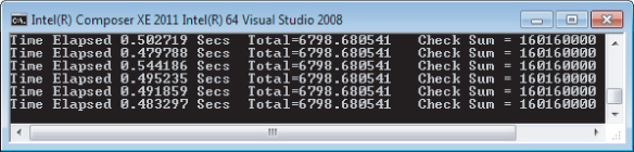
The example application is quite contrived and doesn't solve any particular problem. Its only purpose is to provide some code that you can optimize and see an improvement in performance as you perform each optimization step. Figure 4.1 shows the output of the program. As you can see, the output is very similar to the application used in Chapter 3 — the main difference being that the Total and Check sum displayed are different values from that chapter.
Figure 4.1 Output of the example application
In addition to using the code example in Listing 4.5, you might like to try applying the seven optimization steps to your own code or from code in one of the case studies (Chapters 13 through 18). You may find that some optimization steps deliver significant performance improvements, whereas other steps may actually slow down your application.
The results shown in this chapter were from three different machines:
- Core 2 laptop — Lenovo T66, Intel Core 2 Duo CPU, T7300 @ 2.00 GHz, 2GB RAM.
- Sandy Bridge laptop — Lenovo W520, Intel Core i7-2820QM @ 2.30 GHz, 8GB RAM. This machine is used to give two sets of results, one with Intel Turbo Boost Technology 2.0 enabled, and one without.
- Xeon workstation — OEM, Intel Xeon CPU, X5680 @ 3.33 GHz (2 processors, 12GB RAM).
![]()
Optimizing Code in Seven Steps
Figure 4.2 shows the steps followed in this chapter, which are based on the Quick-Reference Guide to Optimization (which you can find at http://software.intel.com/sites/products/collateral/hpc/compilers/compiler_qrg12.pdf).
Figure 4.2 The seven optimization steps
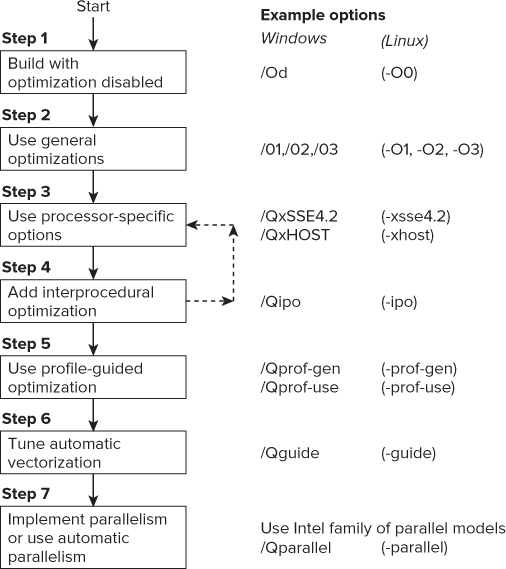
In the first step you build the application with no optimization. You do this to make sure that your program works as expected. Sometimes an optimization step can break the application, so it's prudent to start with an unoptimized application. Once you are confident that no errors exist in your program, it's okay to go to the next step.
Figure 4.2 shows the Windows and Linux versions of the options used in this chapter. In most of the text of this chapter the Windows version of the options is used, but they can be substituted with the Linux options.
![]()
Using the Compiler's Reporting Features
For each optimization step, the Intel compiler can generate a report that is useful for gleaning what optimizations the compiler has carried out:
- Optimization report — Use the /Qopt-report option, as described in the section “Step 2: Use General Optimizations.”
- Auto-Vectorization report — Use the /Qvec-report option, as described in the section “Step 3: Use Processor-Specific Optimizations.”
- Auto-Parallelism report — Use the /Qpar-report option, as described in Chapter 6, “Where to Parallelize.”
- Guided Auto-Parallelism report — Use the /Qguide option, as described in the section “Step 6: Tune Auto-Vectorization.”
Step 1: Build with Optimizations Disabled
Before doing any optimization you should ensure that the unoptimized version of your code works. On very rare occasions optimizing can change the intended behavior of your applications, so it is always best to start from a program you know builds and works correctly.
The /Od (-O0) option actively stops any optimizations from taking place. It generally is used while the application is being developed and inspected for errors. Single-stepping through code with a debugger is much easier with programs built at /Od. If you ever end up having to look at the assembler code the compiler generates, it is much easier to understand the output from /Od than from some of the other options.
Table 4.2 shows the results of building the application with optimizations disabled using the /Od option as well as the default build (/O2). The program has a loop that executes six times, printing the time each iteration took. The table records the lowest value.
Table 4.2 Results of Running the /Od and /O2 Builds
| Build Machine | /Od | /O2 |
| Core 2 laptop | 3.041 | 0.474 |
| Sandy Bridge | 2.164 | 0.293 |
| Sandy Bridge (with Turbo Boost) | 1.588 | 0.211 |
| Xeon workstation | 1.325 | 0.238 |
If you are benchmarking on a machine that supports Turbo Boost Technology, it is better that you disable it in the computer's BIOS before proceeding. When Turbo Boost Technology is turned on, the clock speed of the CPU can dynamically change, depending on how busy the CPU is, which can distort the results. Of course, you should turn it back on again at the end.
Another technology that can lead to an inconsistent set of benchmarks is Intel Hyper-Threading Technology. When hyper-threading is enabled, the processor looks as though it has twice as many cores as it really has. This is done by sharing the execution units and using extra electronics that save the state of the various CPU registers. One side effect of using hyper-threading is that the results of your benchmarks can be distorted as the different hyper-threads contend for resources from the execution units.
Many optimization practitioners choose to turn off both Turbo Boost Technology and Hyper-Threading Technology so that they get more consistent results in the different stages of tuning. You should be able to disable both technologies in the BIOS of your PC. See your PC's handbook for instructions.
The Intel compiler assumes that you are building code for a computer that can support SSE2 instructions. If you are building for a very old PC (for example, a Pentium 3), you will need to add the option /arch32 (Windows) or -mia32 (Linux) for your code to run successfully. Architecture-specific options are discussed more in the section “Step 3: Use Processor-Specific Optimizations.”
You can try out this first step for yourself in Activity 4-1.
Setting Up the Build Environment
- On Windows, open an Intel compiler command prompt. The path to the command prompt will be similar to the following. (The exact names and menu items will vary, depending on which version of Parallel Studio and Visual Studio you have installed.)
Start ⇒ All Programs ⇒ Intel Parallel Studio XE 2011 ⇒ Command Prompt ⇒ Intel64 Visual Studio Mode
- On Linux, make sure the compiler variables have been sourced:
$ source /opt/intel/bin/compilervars.sh intel64
If you are running a 32-bit operating system, the parameter passed to the compilervars.sh file should be ia32.
Building and Running the Program
- Linux
make clean
make TARGET=intel.noopt CFLAGS= -O0 (Note : this is a capital ‘O’
followed by zero)
- Windows
nmake clean
nmake TARGET=intel.noopt CFLAGS=/Od
Step 2: Use General Optimizations
Table 4.3 describes four course-grained optimization switches: /O1, /O2, /O3, and /Ox. These switches are a good starting point for optimizing your code. Each option is progressively more aggressive at the optimizations it applies. The option /O1 generates smaller code than the other options. When you call the compiler without any switches, the compiler defaults to using /O2.
![]()
Table 4.3 The General Optimization Switches
| Option | Description |
| /O1 (-O1) | Optimizes for speed and size. This option is very similar to /O2 except that it omits optimizations that tend to increase object code size, such as the inlining of functions. The option is generally useful where memory paging due to large code size is a problem, such as server and database applications.
Note that auto-vectorization is not turned on at /O1, even if it is invoked individually by its fine-grained switch /Qvec. However, at /O1 the vectorization associated with array notations is enabled. |
| /O2 (-O2) | Optimizes for maximum speed. This option creates faster code in most cases. Optimizations include scalar optimizations; inlining and some other interprocedural optimizations between functions/subroutines in the same source file; vectorization; and limited versions of a few other loop optimizations, such as loop versioning and unrolling that facilitate vectorization. |
| /O3 (-O3) | Optimizes for further speed increases. This includes all the /O2 optimizations, as well as other high-level optimizations, including more aggressive strategies such as scalar replacement, data pre-fetching, and loop optimization, among others. |
| /Ox (Windows only) | Full optimization. This option generates fast code without some of the fine-grained option strategies adopted by /O2. |
Using the General Options on the Example Application
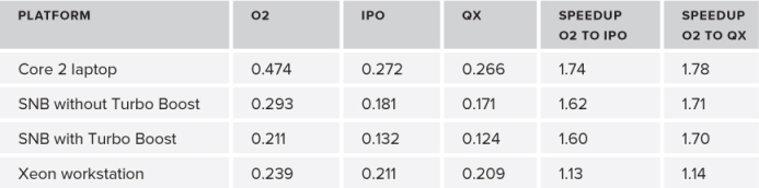
Figure 4.3 shows the results of running the example application on the four target platforms.
- The option /O1, an option designed to produce smaller code, runs slower than the other options.
- There is no difference between the performance of the /O2 option and the more aggressive /O3 or /Ox options.
Figure 4.3 The results of running the example application
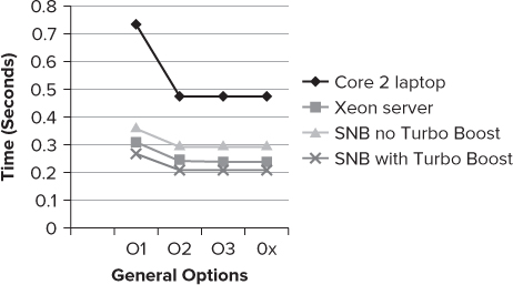
There is no guarantee that the more aggressive optimization options will result in your application running faster. In the case of the example application, /O2 seems the best choice.
Generating Optimization Reports Using /Qopt-report
The compiler can produce reports on what optimizations were carried out. By default, these reports are disabled. Enabling the reports can sometimes help you identify whether a piece of code has been optimized. Note that the coarse- and fine-grained options you use determine which optimizations are applied, including auto-vectorization. If auto-parallelization is also turned on by /Qparallel, messages about auto-parallelizing of loops are also included. You can read more about auto-parallelism and the /Qparallel option in Chapter 6, “Where to Parallelize.”
Reducing the Size of the Report
Using /Qopt-report on its own can result in a fairly large report. To reduce the size of the report, you can:
- Control the level of detail by using /Qopt-report: n, where n is a number between 0 and 3.
- 0 — No reports.
- 1 — Tells the compiler to generate reports with minimum level of detail.
- 2 — Tells the compiler to generate reports with medium level of detail. This is the default level of reporting when this option is not included on the command line.
- 3 — Tells the compiler to generate reports with maximum level of detail.
- Select which phases to have a report on by using the /Qopt-report-phase option.
- Limit the report to specific functions by using the /Qopt-report-routine:<string> option.
Table 4.4 shows the different phases used with the /Qopt-report-phase option.
Table 4.4 Phase Names Used in Report Generation
| Phase | Description |
| ipo_inl | Gives an inlining report from the interprocedural optimizer |
| hlo | Reports on high-level optimization (HLO), including loop and memory optimizations |
| hpo | Reports on high-performance optimization (HPO), including auto-vectorization and auto-parallelization optimizations |
| pgo | Reports on profile-guided optimizations |
Creating Focused Reports
Each phase in Table 4.4 is a collection of even smaller reports — too many to describe here. If you are interested in just one specific phase, you can generate one of these smaller reports using the option /Qopt-report-phase. Running the option /Qopt-report-help as follows brings up a list of all the phases available:
icl /Qopt-report-help
Intel(R) C++ Intel(R) 64 Compiler XE for applications running on Intel(R) 64,
Version 12.0.3.175 Build 20110309
Copyright (C) 1985-2011 Intel Corporation. All rights reserved.

Intel(R) Compiler Optimization Report Phases
usage:  -Qopt_report_phase <phase>

ipo, ipo_inl, ipo_cp, ipo_align, ipo_modref, ipo_lpt, ipo_subst, ipo_ratt, ipo_vaddr,
ipo_pdce, ipo_dp, ipo_gprel, ipo_pmerge, ipo_dstat, ipo_fps, ipo_ppi, ipo_unref, ipo_wp,
ipo_dl, ipo_psplit, ilo, ilo_arg_prefetching, ilo_lowering, ilo_strength_reduction,
ilo_reassociation, ilo_copy_propagation, ilo_convert_insertion, ilo_convert_removal,
ilo_tail_recursion, hlo, hlo_fusion, hlo_distribution, hlo_scalar_replacement,
hlo_unroll, hlo_prefetch, hlo_loadpair, hlo_linear_trans, hlo_opt_pred, hlo_data_trans,
hlo_string_shift_replace, hlo_ftae, hlo_reroll, hlo_array_contraction,
hlo_scalar_expansion, hlo_gen_matmul, hlo_loop_collapsing, hpo, hpo_analysis,
hpo_openmp, hpo_threadization, hpo_vectorization, pgo, tcollect, offload, all
After using the general optimizations, the next step is to experiment with processor-specific optimization. Before doing that, however, try out the general optimizations by completing Activity 4-2.
- Linux
make clean
make CFLAGS="-O1" TARGET="intel.O1"
- Windows
nmake clean
nmake CFLAGS="/O1" TARGET="intel.O1"
Step 3: Use Processor-Specific Optimizations
Auto-vectorization is one of the most significant contributions the Intel compiler makes to getting really fast code. Four points need to be made straight away:
- When you use the compiler out of the box (that is, the default behavior), auto-vectorization is enabled, supporting SSE2 instructions. This is safe to use on all but the very oldest Intel and non-Intel devices.
- You can enhance the optimization of auto-vectorization beyond the default behavior by explicitly using some additional options. In the following example, the example application is rebuilt to support AVX instructions, leading to a 10 percent improvement when the application is run on the Sandy Bridge laptop.
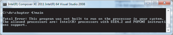
- If you run an application on a CPU that does not support the level of auto-vectorization you chose when it was built, the program will fail to start. The following error message will be displayed: This program was not built to run on the processor in your system.
- You can get the compiler to add multiple paths in your code so that your code can run on both lower- and higher-spec CPUs, thus avoiding the risk of getting an error message or program abort. This topic is covered later in this chapter in “Building Applications to Run on More Than One Type of CPU.”
What Is Auto-Vectorization?
Auto-vectorization makes use of the SIMD (Single Instruction Multiple Data) instructions within the processor to speed up execution times. The original SIMD instructions, MMX (MultiMedia eXtensions), were written for special 64-bit registers resident within the processor. This has been superseded by the SSE (Streaming SIMD Extension), which was first introduced in 1999 and operated on 128-bit floating-point registers. Figure 4.4 shows the innovations in SIMD from then until the present date.
Figure 4.4 The SIMD timeline

SIMD instructions operate on multiple data elements in one instruction using the extrawide SIMD registers. The Intel compiler uses these SIMD instructions to apply auto-vectorization to loopy code. Consider the following code snippet:
#define MAX 1024
float x[MAX];
float y[MAX];
float z[MAX];
for(i = 0; i <= MAX; i++)
  z[i] = x[i] + y[i];
Without auto-vectorization, the compiler produces a separate set of instructions that does the following for each iteration of the loop:
- Reads x[i] and y[i] for the current loop iteration
- Adds them together
- Writes the results in z[i] for the current loop iteration
Array z would be updated 1,024 times. The compiler might even use SSE scalar instructions — that is, instructions that operate on one data item at a time.
If auto-vectorization is enabled, the compiler will use SSE packed instructions rather than scalar instructions. Figure 4.5 shows a scalar and a packed instruction. The first instruction, addss, is a scalar instruction that adds x1 to y1. One calculation is performed on one data item.
Figure 4.5 An example of scalar and packed SSE instructions
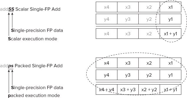
The second instruction, addps, is a packed (or vector) instruction that adds x1, x2, x3, and x4 to y1, y2, y3, and y4. One calculation is performed simultaneously on four data items.
By applying the auto-vectorizer to the preceding code snippet, the compiler can reduce the loop count MAX by a factor of four, so only 256 iterations of the loop need be performed, rather than the original 1,024.
Auto-Vectorization Guidelines
To be amenable to auto-vectorization, any loops must follow the following guidelines:
- The loop trip count must be known runtime at loop entry and remain the same for the duration of the loop.
- The loop counter may be a variable as long as that variable is set before the loop starts and remains unchanged during the loop run.
- The loop cannot be terminated within itself or by some data dependency within the loop, because this would imply an inconstant loop count. By the same considerations, the loop must be a single entry-and-exit loop.
- There must be no backward dependencies between iterations of the loop. If the compiler cannot determine that there are no dependencies, it will assume there are and subsequently not vectorize the loop.
- Loops involving overlapping arrays cannot be vectorized because loop dependencies may occur. Usually the compiler can easily determine if declared arrays overlap, because their addresses are constants. The compiler will assume overlapping arrays have loop dependencies unless told otherwise by the programmer. In simple cases, the compiler can test for overlapping arrays at run time.
- There must be no function calls in a loop. However, inlined functions and elemental functions (as used in array notation) will not cause a problem.
Turning On Auto-Vectorization
Auto-vectorization is included implicitly within some of the general optimization options, and implicitly switched off by others. It can be further controlled by the auto-vectorization option /Qvec. Normally, the only reason you would use the /Qvec option would be to disable auto-vectorization (that is, /Qvec-) for the purposes of testing.
Here's the default behavior of the general options:
- The general options /O2, /O3, and /Ox turn on auto-vectorization. You can override these options by placing the negative option /Qvec- directly on the compiler's command line.
- The general options /Od and /O1 turn off auto-vectorization, even if it is specifically set on the compiler's command line by using the /Qvec option.
Enhancing Auto-Vectorization
When auto-vectorization is enabled, the compiler uses the SSE2 instructions, which were introduced in 2000. If your target CPU is more recent, you can get better performance by using the /Qx<architecture> option, where <architecture> can be one of SSE2, SSE3, SSSE3, SSE4.1, SSE4.2, or AVX.
Table 4.5 shows the speed of the example application on the Sandy Bridge laptop with Turbo Boost Technology disabled. Turning on AVX gives a performance boost of a further 9 percent, compared to using the default auto-vectorization.
Table 4.5 Auto-Vectorization Speedup
| Setting | Time | Speedup |
| SSE2 | 0.293 | 1 |
| AVX | 0.270 | 1.09 |
Using the /Qx option to enhance auto-vectorization causes two potential problems. The moment you build an application using the /Qx option, it will not run on a non-Intel CPU. For example, any application built with /Qx will not run on an AMD device. To solve this, you should use the /arch options rather than the /Qx options, described in the following section.
If you run the optimized application on a generation of Intel CPU that does not support the option you used, the application will fail to run. For example, an application built with /QxAVX will not run on a first-generation Intel Core 2 CPU.
Figure 4.6 shows an example of a message you will get if you run an application on hardware that does not support the level of auto-vectorization you have chosen.
Figure 4.6 Running a mismatched application
Building for Non-Intel CPUs
If you intend to run code on Intel and non-Intel devices, you should use the /arch:<architecture> option, where architecture can be ia32, SSE2, SSE3, SSSE3, or SSE4.1.
For example, using the option /arch:SSE4.1 produces an application that will run on any CPU that supports SSE4.1, whether it is an Intel CPU or not.
![]()
Determining That Auto-Vectorization Has Happened
You can get a detailed report from the vectorizer by using the /Qvec-report option. The /Qvec-report n option reports on auto-vectorization, where n can be set from 0 to 5 to specify the level of detail required in the report, as follows:
- n = 0 — No diagnostic information (default if n omitted).
- n = 1 — Reports only loops successfully vectorized.
- n = 2 — Reports which loops were vectorized and which were not (and why not).
- n = 3 — Same as 2 but adds the dependency information that caused the failure to vectorize.
- n = 4 — Reports only loops not vectorized.
- n = 5 — Reports only loops not vectorized and adds dependency information.
When you build the example application with the /Qvec-report1 option, the compiler reports the following:
chapter4.c(64): (col. 5) remark: PERMUTED LOOP WAS VECTORIZED.
series.c(7): (col. 5) remark: LOOP WAS VECTORIZED.
Building with the /Qvec-report4 option gives a list of loops that are not vectorized. Here's a cut-down version of the output:
chapter4.c(54): (col. 5) remark: loop was not vectorized: not inner loop.
… lots more like this

chapter4.c(45): (col. 3) remark: loop was not vectorized: nonstandard loop is not a
vectorization candidate.

chapter4.c(11): (col. 7) remark: loop was not vectorized: existence of
vector dependence.
For a further discussion on these types of failures to vectorize, see the next section, “When Auto-Vectorization Fails.” There's a further development of the auto-vectorized code after IPO has been applied — see the section “The Impact of Interprocedural Optimization on Auto-Vectorization.”
When Auto-Vectorization Fails
The auto-vectorizer has a number of rules that must be fulfilled before vectorization can happen. When the compiler is unable to vectorize a piece of code, the vectorization report will tell you which rules were broken (provided you have turned on the right level of reporting detail — refer to the section “Determining That Auto-Vectorization Has Happened” earlier in this chapter).
Error Messages
Following are some of the main report messages associated with non-vectorization of a loop:
- Low trip count — The loop does not have sufficient iterations for vectorization to be worthwhile.
- Not an inner loop — Only the inner loop of a nested loop may be vectorized, unless some previous optimization has produced a reduced nest level. On some occasions the compiler can vectorize an outer loop, but obviously this message will not then be generated.
- Nonstandard loop is not a vectorization candidate — The loop has an incorrect structure. For example, it may have a trip count that is modified within the loop, or it may contain one or more breakouts.
- Vector dependency — The compiler discovers, or suspects, a dependency between successive iterations of the loop. You can invite the compiler to ignore its suspicions by using the #pragma ivdep directive, provided you know that any vectorization would be safe.
- Vectorization possible but seems inefficient — The compiler has concluded that vectorizing the loop would not improve performance. You can override this by placing #pragma vector always before the loop in question.
- Statement cannot be vectorized — Certain statements, such as those involving switch and printf, cannot be vectorized.
- Subscript too complex — An array subscript may be too complicated for the compiler to handle. You should always try to use simplified subscript expressions.
Organizing Data to Aid Auto-Vectorization
Sometimes auto-vectorization will fail because access to data is not performed consecutively within the vectorizable loop.
You can load four consecutive 32-bit data items directly from memory in a single 128-bit SSE instruction. If access is not consecutive, you need to reorder the code to achieve auto-vectorization.
When working on legacy code that has a lot of nonsequential data items, some programmers write wrapper functions and use intermediate data structures to make auto-vectorization possible.
Non-Unit Strides
Consider the following matrix multiplication example. The nested loop results in access to array c being nonconsecutive (that is, a non-unit stride):
double a[4][4], b[4][4], c[4][4];
for (int j = 0; j < 4; j++)
 for (int i = 0; i <= j; i++)
   c[i][j] = a[i][j]+b[i][j];
The example loops through the rows, which means that the data items in a vector instruction will not be adjacent. The compiler reports the following:
elem2.cpp(15): (col. 3) remark: loop was not vectorized: not inner loop.
elem2.cpp(16): (col. 4) remark: loop was not vectorized: vectorization possible but
seems inefficient.
However, the code can be made to be vectorizable by changing the order in which the data is stored and, therefore, changing the order of the loop:
double a[4][4], b[4][4], c[4][4];
for (int j = 0; j < 4; j++)
 for (int i = 0; i <= j; i++)
   c[j][i] = a[i][j]+b[i][j];
The compiler will now report success:
elem2.cpp(15): (col. 1) remark: loop was not vectorized: not inner loop.
elem2.cpp(16): (col. 2) remark: LOOP WAS VECTORIZED.
Notice that arrays a and b are still accessed by row, and hence non-unit strides.
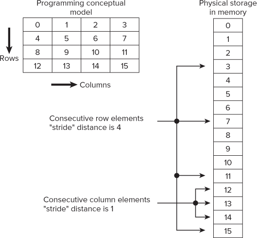
Figure 4.7 shows how a two-dimensional array has its columns stored consecutively in memory, but its row elements are stored in memory with a gap (or stride) between each. By iterating through such an array by columns, rather than by rows, vectorization becomes possible.
Figure 4.7 Stride values when accessing a two-dimensional array
Structure of Arrays vs. Arrays of Structures
The simplest data structure in use is the array, which contains a contiguous collection of data items that can be accessed by an ordinal index, making it ideal for vectorizing. Data organized as a structure of arrays (SOA) are also ideal candidates for vectorizing because it is still being done at the array level. However, data organized as an array of structures (AOS), although an excellent format for encapsulating data, is a poor candidate for vector programming.
Helping the Compiler to Vectorize
To ensure correct code generation, the compiler treats any assumed dependencies as though they were proven dependencies, which prevents vectorization. The compiler always assumes a dependency where it cannot prove that it is not a dependency. However, if you are certain that a loop can be safely vectorized and any dependencies ignored, the compiler can be informed in the following ways.
Using #pragma ivdep
One way of informing the compiler that there are no dependencies within a loop is to place #pragma ivdep just before the loop. The pragma applies only to the single following loop, not all the following loops. Note that the compiler will ignore only assumed dependencies; it won't ignore any that it can prove. Use #pragma ivdep only when you know that the assumed loop dependencies are safe to ignore.
The following example will not vectorize without the ivdep keyword if the value of k is unknown, because it may well be negative:
             #pragma ivdep
             for(int i = 0;i < m; i++)
                 a[i] = a[i + k] * c;
Using the restrict Keyword
Another way to override assumptions concerning overlapping arrays is to use the restrict keyword on pointers when declaring them. The use of the restrict keyword in pointer declarations informs the compiler that it can assume that during the lifetime of the pointer only this single pointer has access to the data addressed by it — that is, no other pointers or arrays will use the same data space. Normally, it is adequate to just restrict pointers associated with the left-hand side of any assignment statement, as in the following code example. Without the restrict keyword, the code will not vectorize.
void f(int n, float *x, float *y, float *restrict z, float *d1, float *d2)
{
  for (int i = 0; i < n; i++)
    z[i] = x[i] + y[i]-(d1[i]*d2[i]);
}
The restrict keyword is part of the C99 standard, so you will have to either enable C99 in the compiler (using /Qstd:c99) or use the /Qrestrict option to force the compiler to recognize the restrict keyword.
Using #pragma vector always
The compiler will not vectorize if it thinks there is no advantage in doing so, issuing the message:
C:Multiplicity.CPP(11): (col. 5) remark: loop was not vectorized: vectorization
possible but seems inefficient
If you want to force the compiler to vectorize a loop, place #pragma vector always immediately before the subsequent loop in the program, as in the following code:
void vec_always(int *a, int *b, int m)
{
  #pragma vector always
    for(int i = 0; i <= m; i++)
      a[32*i] = b[99*i];
}
Again, it applies only to the loop that follows; its use instructs the compiler to vectorize the following loop, provided it is safe to do so. You can use #pragma vector always to override any efficiency heuristics during the decision to vectorize or not, and to vectorize non-unit strides or unaligned memory accesses. The loop will be vectorized only if it is safe to do so. The outer loop of a nest of loops will not be vectorized, even if #pragma vector always is placed before it.
Using #pragma simd
You can use #pragma simd to tell the compiler to vectorize the single loop that follows. This option is more dangerous than the other vectorization pragmas because it forces the compiler to vectorize a loop, even when it is not safe to do so. This complements, but does not replace, the fully automatic approach. You can use #pragma simd with a selection of clauses, including:
- vectorlength (n1[,n2]… ), where n is a vector length, which must be an integer of value 2, 4, 8, or 16. If more than one integer is specified, the compiler will choose from them.
- private (var1[,var2]… ), where var must be a scalar variable. Private copies of each variable are used within each iteration of the loop. Each copy takes on any initial value the variable might have before entry to the loop. The value of the copy of the variable used in the last iteration of the loop gets copied back into the original variable. Multiple clauses get merged as a union.
- linear (var1:step1[,var2:step2] … ), where var is a scalar variable and step is a compile-time positive integer constant expression. For each iteration of a scalar loop, var1 is incremented by step1, var2 is incremented by step2, and so on. Multiple clauses get merged as a union.
- reduction (oper:var1[,var2] … ), where oper is a reduction operator, such as +, -, or *, and var is a scalar variable. The compiler applies the vector reduction indicated by oper to the variables listed in a similar manner to that of the OpenMP reduction clause.
- [no]assert, which directs the compiler to assert (or not to assert) when the vectorization fails. The default is noassert. Note that using assert turns failure to vectorize from being a warning to an error.
![]()
Following is an example using #pragma simd:
#pragma simd private(b)
for( i=0; i<MAXIMUS; i++ )
{
  if( a[i] > 0 )
  {
    b = a[i];
    a[i] = 1.0/a[i];
  }
  if( a[i] > 1 )a[i] += b;
}
The compiler will report success with the following message:
C:Multiplicity.cpp(42): (col. 4) remark: SIMD LOOP WAS VECTORIZED.
Placing the negative option /Qsimd- on the compiler command line disables any #pragma simd statements in the code.
Using #pragma vector [un]aligned
The compiler can also write more efficient code if aligned data is used, starting either on 32-bit boundaries in the case of IA-32 processors, or 64-bit boundaries for 64-bit processors. If the compiler cannot decide if a data object is aligned, it will always assume it is unaligned. Coding for unaligned data is less efficient than coding for aligned data. You can always override the failsafe tendencies of the compiler by using the following two pragmas:
- #pragma vector aligned — Instructs the compiler to use aligned data movement instructions for all array references when vectorizing.
- #pragma vector unaligned — Instructs the compiler to use unaligned data movement instructions for all array references when vectorizing.
All code following the use of #pragma vector aligned is assumed to be aligned; likewise, all code following the use of #pragma vector unaligned is assumed to be unaligned. By using these pragmas, you can tell the compiler that different parts of your code can be assumed to use aligned or unaligned data. If you use the aligned pragma on an unaligned SSE data access, it is likely to result in failure. This is not the case for AVX.
You can align data by using _declespec(align) or the _mm_malloc() SSE-intrinsic function, as follows:
// align data to 32-byte address
_declepec(align(32)) double data[15];

// Allocate 100 bytes of memory; the start address is aligned to 16 bytes
double *pData = (double *)_mm_malloc(100,16);

// free the memory
_mm_free(pdata);
The call to _mm_malloc() results in the allocation of 100 bytes of memory that is aligned to a 16-byte address, which is later deallocated using the function _mm_free().
Controlling the Default Auto-Vectorization Options
- Linux
make clean
make TARGET=default
.default.exe
- Windows
nmake clean
nmake TARGET=default
default.exe
- Linux
make clean
make CFLAGS="-vec-" TARGET=novec
.
ovec.exe
- Windows
nmake clean
nmake CFLAGS="/Qvec-""TARGET=novec
novec.exe
The two executables from steps 1 and 2 should run at different speeds.
Enhancing the Auto-Vectorization Options
- Linux
make clean
make CFLAGS="-xSSE2" TARGET=intel.SSE2
.intel.SSE2.exe
- Windows
nmake clean
nmake CFLAGS="-/QxSSE2" TARGET=intel.SSE2
intel.SSE2.exe
Creating a Portable Application
- Linux
make clean
make CFLAGS="-axAVX" TARGET=intel.axAVX
.intel.axAVX.exe
- Windows
nmake clean
nmake CFLAGS="-/QaxAVX" TARGET=intel.axAVX
intel.axAVX.exe
Step 4: Add Interprocedural Optimization
Interprocedural optimization (IPO) performs a static, topological analysis of an application. With the option /Qip the analysis is limited to occur within each source file. With the option /Qipo the analysis spans across all the source files listed on the command line. IPO analyzes the entire program and is particularly successful for programs that contain many frequently used functions of small and medium length. IPO reduces or eliminates duplicate calculations and inefficient use of memory, and simplifies loops.
Other optimizations carried out include alias analysis, dead function elimination, unreferenced variable removal, and function inlining to be carried out across source files. IPO can reorder the functions for better memory layout and locality. In some cases, using IPO can significantly increase compile time and code size.
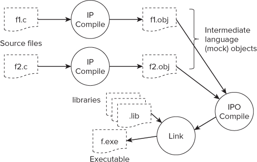
Figure 4.8 shows how the compiler performs IPO. First, each individual source file is compiled, and an object file is produced. The object files hold extra information that is used in a second compilation of the files. In this second compilation, all the objects are read together, and a cross-file optimization is performed. The output from this second pass is one or more regular objects. The linker is then used to combine the regular objects with any libraries that are needed, producing the final optimized application.
Figure 4.8 Interprocedural optimization
During build time you can control the number of object files created from the multiple source files by using the option /Qipo<n>, where n is the number of object files to be created. If n is zero or is omitted (the default), the compiler is left to decide how many objects are created. For large programs several object files may be created; otherwise, just one. The maximum number of object files that can be created is one for each source file.
Adding Interprocedural Optimization to the Example Application
The fourth column of Table 4.6 gives the results of using IPO on the example application. As you can see, there is more than a 60 percent speedup on three of the platforms when comparing an /O2 build with a /Qipo build.
Table 4.6 The Results of Using IPO with /O2 and /QhHost
If you are using Microsoft Visual Studio, rather than the command line, you will find that /Qipo is already enabled in the release build of your project.
The Impact of Interprocedural Optimization on Auto-Vectorization
The Quick-Reference Guide to Optimization recommends that you carry out IPO after using any processor-specific options. The truth is that in many cases auto-vectorization will bring better results after IPO has been applied. However, experience shows that using IPO is sometimes difficult to achieve, so for pragmatic reasons IPO has been placed later in the optimization cycle. In this book we have the luxury of being able to spend a few more words explaining the issues — hence, the extra feedback arrow that was introduced in Figure 4.2.
IPO introduces extra time and complexity into the build process. Occasionally the compiler can run out of memory or slow down to such a pedestrian pace that the developer gets impatient and abandons IPO. On some large projects, it is impossible to successfully complete an IPO session. Because of these potential difficulties, IPO has been placed after some of the easier-to-handle optimizations in the optimization steps. One downside of doing this is that code presented to the auto-vectorizer will not have had the benefit of IPO, especially the cross-file function inlining.
If it's not practical to use the /Qipo option in your build environment, try using /Qip, which does IPO just within the single files.
IPO Improves Auto-Vectorization Results of the Example Application
If you find that your project will run IPO successfully, it is worthwhile to apply the auto-vectorization options again, especially if you have already ruled out one of the higher specification options because you saw no difference in performance. The sixth column of Table 4.6 shows the impact of using IPO on the example application when enhanced auto-vectorization has been used. For each build, the highest SIMD instruction set that the CPU could support was used.
IPO Brings New Auto-Vectorization Opportunities
It is also worth getting a fresh vectorization report to see what new things turn up. In the previous step, when the vectorization reports were generated, they were generated for each individual file at compilation time. Once /Qipo is used, the report generation is delayed until the final cross-file compilation.
Building with the /Qvec-report3 option gives a list of loops that were not vectorized. What is interesting is that both new failures and new successes are reported for line 51:
chapter4.c(51): (col. 11) remark: LOOP WAS VECTORIZED.
. . .
chapter4.c(51): (col. 11) remark: loop was not vectorized: not inner loop.
chapter4.c(51): (col. 11) remark: loop was not vectorized: not inner loop.
chapter4.c(51): (col. 11) remark: loop was not vectorized: existence of vector
dependence.
The reason for more than one vectorization activity being reported on a single line is that the use of /Qipo has resulted in several of the functions being inlined. You effectively have a triple-nested loop at line 51. This line has a call to the work() function. The following code snippet shows the nested loop within the work() function that calls the Series1() and Series2() functions:
for (i=0;i<N;i++){
    for (j=0;j<N;j++) {
      sum += 1;
      // Calculate first Arithmetic series
      sumx= Series1(j);

      // Calculate second Arithmetic series
      sumy= Series2(j);

      // initialize the array
      if( sumx > 0.0 )*total = *total + 1.0 / sqrt( sumx );
      if( sumy > 0.0 )*total = *total + 1.0 / sqrt( sumy );
      a[N*i+j] = *total;
    }
  }
The effect of /Qipo inlining means that the most deeply nested loops associated with line 51 come from Series1()and Series2():
double Series1(int j)
{
  int k;
  double sumx = 0.0;
    for( k=0; k<j; k++ )
      sumx = sumx + (double)k;
  return sumx;
}

double Series2(int j)
{
  int k;
  double sumy = 0.0;
  for( k=j; k>0; k--,sumy++ )
    sumy = AddY(sumy, k);
  return sumy;
}
The two messages about the loop not being an inner loop refer to the two loops in work.c, which have become outer loops as a result of the inlining. The question is, what is the loop-dependency message referring to? One way to find out which message refers to which loop is to comment out the call to Series1() and Series2() in turn and see which messages disappear from the vectorization report. After experimenting, it is clear that the call to Series2() is the cause of the vector-dependency message. By commenting out the sumy++ in the loop and the sumy-- in the AddY()function, the dependency is removed, as shown in Listing 4.1.
 Listing 4.1: Modifications to the AddY function
series.c
double Series2(int j)
{
  int k;
  double sumy = 0.0;
  for( k=j; k>0; k--)
  {
    // sumy++;
    sumy = AddY(sumy, k);
  }
  return sumy;
}
addy.c
double AddY( double sumy, int k )
{
// sumy--;
sumy = sumy + (double)k;
  return sumy;
}
code snippet Chapter44-1series.c and addy.c
Making the preceding changes has a positive impact on performance, improving it by an additional 20 percent.
You can try out IPO for yourself in Activity 4-4.
- Linux
make clean
make CFLAGS="-ipo" TARGET="intel.ipo.exe"
.intel.ipo.exe
- Windows
nmake clean
nmake CFLAGS="/Qipo" TARGET="intel.ipo.exe"
intel.ipo.exe
- Linux
make clean
make CFLAGS="-ipo -xAXV" TARGET="intel.ipo.xavx.exe"
.intel.ipo.xavx.exe
- Windows
nmake clean
nmake CFLAGS="/Qipo /QxAVX" TARGET="intel.ipo.xavx.exe"
intel.ipo.xavx.exe
Step 5: Use Profile-Guided Optimization
So far, all the optimization methods described have been static — that is, they analyze the code without running it. Static analysis is good, but it leaves many questions open, including:
- How often is variable x greater than variable y?
- How many times does a loop iterate?
- Which part of the code is run, and how often?
Benefits of Profile-Guided Optimization
PGO uses a dynamic approach. One or more runs are made on unoptimized code with typical data, collecting profile information each time. This profile information is then used with optimizations set to create a final executable.
Some of the benefits of PGO include:
- More accurate branch prediction
- Basic code block movements to improve instruction cache behavior
- Better decision of functions to inline
- Can optimize function ordering
- Switch-statement optimizer
- Better vectorization decisions
The Profile-Guided Optimization Steps
Carrying out PGO involves three steps, as shown in Figure 4.9.
- Windows — icl /Qprof-gen prog.c
- Linux — icc -prof-gen prog.c
- Windows — icl /Qprof-use prog.c
- Linux — icc -prof-use prog.c
Figure 4.9 The three steps to using PGO
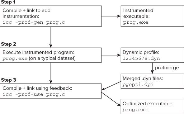
PGO uses the results of the test runs of the instrumented program to help apply the final optimizations when building the executable. For example, the compiler can decide whether a function is worth inlining by using the profile feedback information to establish how often the function is called.
The various .dyn files are averaged to produce a single version, which is then used. After step 3 has completed, the files are deleted.
Table 4.7 shows the different options that you can use in PGO.
Table 4.7 PGO Compiler Options
| Linux | Windows | Description |
| -prof-gen | /Qprof-gen | Adds PGO instrumentation, which creates a new .dyn file every time the instrumented application is run |
| -prof-use | /Qprof-use | Uses collected feedback from all the .dyn files to create the final optimized application |
| -prof-gen=srcpos | /Qprof-gen:srcpos | Creates extra information for use with the Intel code coverage tool |
| -opt-report-phase=pgo | /Qopt-report-phase:pgo | Creates a PGO report |
Table 4.8 shows the results of using PGO on four different platforms.
- Linux
make reallyclean
make CFLAGS="-prof-gen" TARGET="intel.pgo.gen.exe"
- Windows
nmake reallyclean
nmake CFLAGS="/Qprof-gen" TARGET="intel.pgo.gen.exe"
Notice the reallyclean target, which deletes any intermediate PGO files that might be lying around.
- Linux
make clean
make CFLAGS="-prof-use" TARGET="intel.pgo.exe"
- Windows
nmake clean
nmake CFLAGS="/Qprof-use" TARGET="intel.pgo.exe"
// initialize matrix b;
    for (i = 0; i < N; i++) {
      for (j=0; j<N; j++) {
        for (k=0;k<DENOM_LOOP;k++) {
                sum += m/denominator;
        }
        b[N*i + j] = sum;
      }
    }
Table 4.8 The Results of Using PGO

The Results
Figure 4.10 shows the results from the various steps applied to the example application in Listing 4.5. The application was run on the Sandy Bridge laptop. In each step, new optimizations were incrementally added using the compiler options. The result labeled “Fix” is where the code in Series2.c was modified.
Figure 4.10 Applying all the optimization steps results in a speedup of more than 300 percent
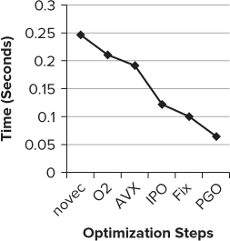
If the application had been built with just the default options, the application would have run at the /O2 setting, giving a run time of 0.211 seconds. At the PGO step, the final speed was 0.064 seconds, giving an impressive speedup of 3.3.
Step 6: Tune Auto-Vectorization
The auto-vectorizer in the Intel compiler expects a certain standard of code. You can use the compiler's reporting features to tell you when the compiler was unable to auto-vectorize. The section “When Auto-Vectorization Fails” covers many of the rules and error messages that can help you understand what the compiler is doing. In addition to the compiler's reporting features, you can also use the GAP option to give you additional advice. Table 4.9 lists some of the differences between the GAP and vectorizer reports.
Table 4.9 Differences Between GAP and Vectorizer Reports
| Feature | Vectorizer Reports | GAP |
| Executable or usable object produced | Y | N |
| Performs application-wide analysis | N | Y |
| Detects breaking of vectorization rules | Y | Y |
| Gives advice on what to do | N | Y |
It is best that you do not use both /Qguide and /Qvec-report at the same time, because this can lead to confusion; rather, use them sequentially after each other. Don't be tempted to skip one of these reports, because experience shows that there will be occasions when the vectorizer will emit a message but the GAP option will not give any specific advice.
GAP gives advice on auto-vectorization and auto-parallelization. This section considers only tuning auto-vectorization; Chapter 6, “Where to Parallelize,” discusses using GAP for auto-parallelism.
Activating Guided Auto-Parallelization
You can activate GAP by using the following option switch:
/Qguide=n
where n can be set from 1 to 4, as follows:
The higher the value of n, the deeper the analysis and the longer it takes.
While the GAP option is set, the compiler will not build an executable; it runs in advisor mode only, generating diagnostic messages telling you how you can improve the code. After making any changes you feel happy with, you need to recompile the application without the /Qguide option to produce an executable file.
![]()
An Example Session
Listing 4.2 is an example session that uses both /Qguide and /Qvec-report options.
Listing 4.2: Sample code suitable for vectorization
void f(int n, float *x, float *y, float *z, float *d1, float *d2)
{
  for (int i = 0; i < n; i++)
    z[i] = x[i] + y[i] – (d1[i]*d2[i]);
}
code snippet Chapter44-2.cpp
The following steps show what output the auto-vectorizer and GAP produces when you compile Listing 4.2:
icl /c test.cpp /Qvec-report2 /c

C:dvguide	est.cpp(3): (col. 3) remark: loop was not vectorized: existence of
vector dependence.
icl /c test.cpp /Qguide /c

test.cpp
GAP REPORT LOG OPENED ON Thu Aug 25 18:33:06 2011

remark #30761: Add -Qparallel option if you want the compiler to generate
recommendations for improving auto-parallelization.

C:dvguide	est.cpp(3): remark #30536: (LOOP) Add -Qno-alias-args option for better
type-based disambiguation analysis by the compiler, if appropriate (the option will
apply for the entire compilation). This will improve optimizations such as vectorization
for the loop at line 3. [VERIFY] Make sure that the semantics of this option is obeyed
for the entire compilation. [ALTERNATIVE] Another way to get the same effect is to add
the "restrict" keyword to each pointer-typed formal parameter of the routine "f".
This allows optimizations such as vectorization to be applied to the loop at line 3.
[VERIFY] Make sure that semantics of the "restrict" pointer qualifier is satisfied:
in the routine, all data accessed through the pointer must not be accessed through
any other pointer. Number of advice-messages emitted for this compilation session: 1.
END OF GAP REPORT LOG
icl /c test.cpp /Qguide /Qno-alias-args

test.cpp
GAP REPORT LOG OPENED ON Thu Aug 25 19:01:29 2011

remark #30761: Add -Qparallel option if you want the compiler to generate
recommendations for improving auto-parallelization.

Number of advice-messages emitted for this compilation session: 0.
END OF GAP REPORT LOG
icl /c test.cpp /Qvec-report2 /Qno-alias-args
test.cpp
C:dvguide	est.cpp(3): (col. 3) remark: LOOP WAS VECTORIZED.
Presto, you have a vectorized loop!
More on Auto-Vectorization
Two additional vectorization-related topics are worth examining:
- Building applications that will safely run on different CPUs
- Other ways of inserting vectorization into your code
Building Applications to Run on More Than One Type of CPU
First, a gentle reminder: If you build an application and use just the general options, or no options at all, then any vectorized code will run on all CPUs that support SSE2. Default builds are safe!
Once you start enhancing auto-vectorization, the compiler adds CPU-specific code into your application — that is, code that will not run on every CPU.
CPU dispatch (sometimes called multipath auto-vectorization) is a means whereby you can add several coexisting specialized paths to your code. Figure 4.11 illustrates the concept. The compiler generates the specialized paths when you use the /Qax option, rather than the /Qx option. (Notice the extra a.)
Figure 4.11 Multipath auto-vectorization
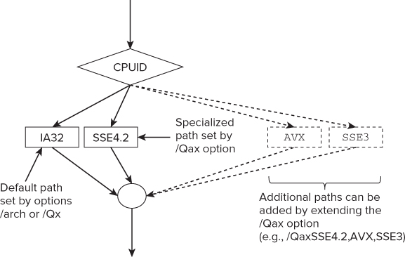
When the code is run, the CPU is first identified using the CPUID instruction. The most appropriate code path is then selected based on the instruction set your CPU can support. When you use the /Qax option, the compiler generates a default path and one or more specialized paths.
You can set the specification of the default path with either the /arch option or the /Qx option. If you think your code will ever be run on a non-Intel CPU, you must not use the /Qx option to create the default path, but rather use the /arch option. For non-Intel devices, the default path is always taken.
Table 4.10 gives some examples of how to use the /Qax option.
Table 4.10 Multipath Vectorization Example
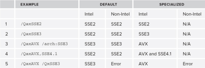
Examples 1 to 4 will run on Intel and non-Intel devices. Example 5 will run only on an Intel device, because the default path has been set up using the /Qx option.
Example 3 is a little more complicated. If the code runs on:
- An Intel device that supports AVX, it will use the AVX specialized path.
- An older Intel device that does not support AVX but still supports SSE3, it will use the default path.
- An older Intel device that supports only SSE2 (or lower), the program will fail to run.
- A non-Intel device that is capable of supporting SSE3 (or higher), it will run on the default path.
- An older non-Intel device that supports only SSE2 (or lower), the program will fail to run.
![]()
Additional Ways to Insert Vectorization
In addition to using auto-vectorization, you can insert vectorization in your code by other means. The ways mentioned in Figure 4.12 range from the fully automatic vectorization to low-level assembler writing. The lower in the diagram, the more difficult it is to do.
Figure 4.12 Other ways of inserting vectorized code
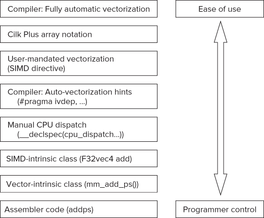
Note the following:
- The vector-intrinsic functions are supported by other compilers as well as the Intel compiler.
- The SIMD-intrinsic classes are C++ classes provided by the Intel compiler. You can see an example of SIMD-intrinsic classes in Chapter 13, “The World's First Sudoku ‘Thirty-Niner.’”
- User-mandated vectorization and auto-vectorization hints are discussed in the section “When Auto-Vectorization Fails.”
- Cilk Plus array notation and manual CPU dispatching are discussed in the following sections, respectively.
Using Cilk Plus Array Notation
Array extensions are a very convenient way of adding vectorized code to your application. When you build an application at optimization level /O1 or higher, the compiler replaces the array notation with vectorized code. If you build with no optimization (/Od), the compiler generates nonvectorized code.
The compiler uses exactly the same rules as for auto-vectorization with respect to which instruction set is used. By default, the compiler uses SSE2 instructions. You can override this behavior by using the /arch, /Qx, or /Qax options.
The Section Operator
Cilk Plus array notation is an extension to the normal C/C++ array notation and is supported by the Intel compiler. A section operator (:) is provided that enables you to express data-parallel operations over multiple elements in an array. The section operator has the format Array[lower bound : length : stride]. Here are some examples:
A[:] // All of array A
B[4:7] // Elements 4 to 10 of array B
C[:][3] // Column 3 of matrix C
D[0:3:2] // Elements 0,2,4 of array D
The first example accesses all the elements of array a[]. The other three examples access arrays B[], C[], and D[] portions as a range, a column, and a stride, respectively.
C/C++ Operators
Most C/C++ operators are available for use on array sections. Each operation is mapped implicitly to each element of the array. Here are two examples of using operators:
z[:] = x[:] * y[:] // element-wise multiplication
c[3:2][3:2] = a[3:2][3:2] + b[5:2][5:2] // 2x2 matrix addition
In the first example, each element of x[] is multiplied by its corresponding element in y[], and the results are written to the corresponding element in z[].
The second example shows that two submatrices are accessed and added and the results placed in another submatrix. The code is equivalent to the following:
c[3][3] = a[3][3] + b[5][5];
c[3][4] = a[3][4] + b[5][6];
c[4][3] = a[4][3] + b[6][5];
c[4][4] = a[4][4] + b[6][6];
The Assignment Operator
The assignment operator (=) applies in parallel every element of the right-hand side to every element of the left-hand side. For example:
a[:][:] = b[:][2][:] + c;
e[:] = d;
The equivalent code for the first example is as follows (assuming array declarations of a[3][3] and b[3][3][3]):
a[0][0] = b[0][2][0] + c;
a[0][1] = b[0][2][1] + c;
a[0][2] = b[0][2][2] + c;
a[1][0] = b[1][2][0] + c;
a[1][1] = b[1][2][1] + c;
a[1][2] = b[1][2][2] + c;
a[2][0] = b[2][2][0] + c;
a[2][1] = b[2][2][1] + c;
a[2][2] = b[2][2][2] + c;
In the second example, the value of d is assigned to every element of array e[].
Reducers
Reducers accumulate all the values in an array using one of nine reducer functions, or alternatively using your own user-defined function. The nine provided reducers are as follows:
- _sec_reduce_add — Adds values
- _sec_reduce_mul — Multiplies values
- _sec_reduce_all_zero — Tests that all elements are zero
- _sec_reduce_all_nonzero — Tests that all elements are nonzero
- _sec_reduce_any_nonzero — Tests that any element is nonzero
- _sec_reduce_max — Determines the maximum value
- _sec_reduce_min — Determines the minimum value
- _sec_reduce_max_ind — Determines index of element with maximum value
- _sec_reduce_min_ind — Determines index of element with minimum value
Here's an example of using the _sec_reduce_add reducer:
// add all elements using a reducer
int sum = _sec_reduce_add(c[:])

// add all elements using a loop
int sum = 0; for(int i = 0;i < sizeof(c);i++){sum += c[i]);
In the first line of code, every element of c[] is added together using the reducer _sec_reduce_add. In the second line, the same operation is performed using a loop.
Elemental Functions
Elemental functions are user-defined functions that can be used to operate on each element of an array. The three steps to writing a function are as follows:
In the following code snippet, the multwo function is applied to each element of array A. At optimization levels /O1 and above, the compiler generates vectorized code for the example.
int _declspec(vector) multwo(int i){return i * 2;}

int main()
{
  int A[100];
  A[:] = 1;
  for (int i = 0 ; i < 100; i++)
    multwo(A[i]);
}
Using Array Notations in the Example Application
The most obvious place to use the array notation is in the multiplication of the matrix in chapter4.c. Listing 4.3 first shows the original code and then the new version.
Listing 4.3: Using array notation in the matrix multiplication
ORIGINAL VERSION
void MatrixMul(double a[N][N], double b[N][N], double c[N][N])
{
  int i,j,k;
  for (i=0; i<N; i++) {
    for (j=0; j<N; j++) {
      for (k=0; k<N; k++) {
        c[i][j] += a[i][k] * b[k][j];
       }
    }
  }
}
VERSION USING ARRAY NOTATION
void MatrixMul(double a[N][N], double b[N][N], double c[N][N])
{
  int i,j;
  for (i=0; i<N; i++) {
    for (j=0; j<N; j++) {
      c[i][j] += a[j][:] * b[:][j];
    }
  }
}
code snippet Chapter44-3.c
By building the application with the /S option, you can examine the assembler code and confirm that the code has been vectorized. The highlighted lines in the following code snippet use a packed multiply double and a packed add double instruction (indicated by the p and d in the instruction's name). Remember that a packed instruction is performing a SIMD operation.
movsd     xmm1, QWORD PTR [r14+r13*8]                   ;14.31
movsd     xmm0, QWORD PTR [r8]                          ;14.10
movhpd    xmm0, QWORD PTR [8+r8]                        ;14.10
unpcklpd  xmm1, xmm1                                    ;14.31
mulpd     xmm1, xmm0                                    ;14.31
movsd     xmm2, QWORD PTR [rdi+r9*8]                    ;14.10
movhpd    xmm2, QWORD PTR [8+rdi+r9*8]                  ;14.10
addpd     xmm2, xmm1                                    ;14.10
Manual CPU Dispatch: Rolling Your Own CPU-Specific Code
Occasionally, developers want to write their own CPU-specific code that they can dispatch manually. The Intel compiler provides two functions to achieve this:
- _declspec(cpu_dispatch(cpuid,cpuid…))
- _declspec(cpu_specific(cpuid))
Listing 4.4 gives an example. First, you should declare an empty function (lines 3 and 4) that must list all the different CPUIDs to be used in the _declspec statement. Table 4.11 shows the valid CPUIDs.
Table 4.11 CPUID Parameters for Manual Dispatching
| Parameter | Architecture |
| core_2nd_gen_avx | Intel AVX |
| core_aes_pclmulqdq | AES |
| core_i7_sse4_2 | SSE4.2 |
| atom | Intel Atom processors |
| core_2_duo_sse4_1 | SSE4.1 |
| core_2_duo_ssse3 | SSSE3 |
| pentium_4_sse3 | SSE3 |
| pentium_4 | Pentium 4 |
| pentium_m | Pentium M |
| pentium_iii | Pentium III |
| generic | Other IA-32 or Intel 64 (Intel and non-Intel) |
Each CPUID declared in the empty function list then needs to have its own CPU-specific function, as shown at lines 7 and 10. The code will also work if the functions have return types rather than void functions. Note that all the CPUIDs, except the generic one, are Intel-specific.
Listing 4.4: Example of manual dispatching
1:  #include <stdio.h>
2:  // need to create specific function versions
3:  _declspec(cpu_dispatch(generic, future_cpu_16))
4:  void dispatch_func() {};
5:
6:  _declspec(cpu_specific(generic))
7:  void dispatch_func() {  printf("Generic
");}
8:
9:  _declspec(cpu_specific(future_cpu_16))
10: void dispatch_func(){ printf("AVX!
");}
11:
12: int main()
13: {
14:   dispatch_func();
15:   return 0;
16: }
code snippet Chapter44-4.c
Source Code
Listing 4.5 contains the source coded for the example application used in this chapter. The code is written in such a way that the different compiler optimizations used in the chapter “make a difference.” As mentioned previously, the code is not an example of writing good optimized code; in fact, some of the code is quite contrived and artificial.
Listing 4.5: The example application
chapter4.c
// Example Chapter 4 example program
#include <stdio.h>
#include <stdlib.h>
#include "chapter4.h"

void MatrixMul(double a[N][N], double b[N][N], double c[N][N])
{
  int i,j,k;
  for (i=0; i<N; i++) {
    for (j=0; j<N; j++) {
      for (k=0; k<N; k++) {
        c[i][j] += a[i][k] * b[k][j];
      }
    }
  }
}
// ***********************************************************************
int main( int argc, char * argv[] )
{
  int i,j,k,l,m;
  long int sum;
  double ret, total;
  int denominator = 2;
  double starttime, elapsedtime;
  double *a,*b,*c;
// -----------------------------------------------------------------------
  m = 2;

  if(argc == 2)
    denominator = atoi(argv[1]);

  // allocate memory for the matrices
  a = (double *)malloc(sizeof (double) * N * N);
  if(!a) {printf("malloc a failed!
");exit(999);}

  b = (double *)malloc(sizeof (double) * N * N);
  if(!b) {printf("malloc b failed!
");exit(999);}

  c = (double *)malloc(sizeof (double) * N * N);
  if(!c) {printf("malloc c failed!
");exit(999);}

  // repeat experiment six times
  for( l=0; l<6; l++ )
  {
    // get starting time
    starttime = wtime();

    // initialize matrix a
    sum = Work(&total,a);

    // initialize matrix b;
    for (i = 0; i < N; i++) {
      for (j=0; j<N; j++) {
        for (k=0;k<DENOM_LOOP;k++) {
          sum += m/denominator;
        }
        b[N*i + j] = sum;
      }
    }

    // do the matrix multiply
    MatrixMul( (double (*)[N])a, (double (*)[N])b, (double (*)[N])c);

     // get ending time and use it to determine elapsed time
    elapsedtime = wtime() - starttime;

    // report elapsed time
    printf("Time Elapsed %03f Secs  Total=%lf   Check Sum = %ld
",
                  elapsedtime, total, sum );
  }
  // return a value from matrix c
  // just here to make sure matrix calc doesn't get optimized away.
  return (int)c[100];
}
// **********************************************************************
work.c
#include "chapter4.h"
#include <math.h>

long int Work(double *total,double a[])
{
  long int i,j,sum;
  double sumx, sumy;
  sum = 0;
  *total = 0.0;

  for (i=0;i<N;i++){
    for (j=0;j<N;j++) {
      sum += 1;
      // Calculate first Arithmetic series
      sumx= Series1(j);

      // Calculate second Arithmetic series
      sumy= Series2(j);

      // initialize the array
      if( sumx > 0.0 )*total = *total + 1.0 / sqrt( sumx );
      if( sumy > 0.0 )*total = *total + 1.0 / sqrt( sumy );
      a[N*i+j] = *total;
    }
  }
  return sum;
}
series.c
extern double AddY( double sumy, int k );

double Series1(int j)
{
  int k;
  double sumx = 0.0;
    for( k=0; k<j; k++ )
      sumx = sumx + (double)k;
  return sumx;
}

double Series2(int j)
{
  int k;
  double sumy = 0.0;
  for( k=j; k>0; k--,sumy++ )
    sumy = AddY(sumy, k);
  return sumy;
}
addy.c
double AddY( double sumy, int k )
{
  sumy = sumy + (double)k -1;
  return sumy;
}
wtime.c
#ifdef _WIN32
#include <windows.h>
double wtime()
{
  LARGE_INTEGER ticks;
  LARGE_INTEGER frequency;
  QueryPerformanceCounter(&ticks);
  QueryPerformanceFrequency(&frequency);
  return (double)(ticks.QuadPart/(double)frequency.QuadPart);
}
#else
#include <sys/time.h>
#include <sys/resource.h>
double wtime()
{
  struct timeval time;
  struct timezone zone;
  gettimeofday(&time, &zone);
  return time.tv_sec + time.tv_usec*1e-6;
}
#endif
chapter4.h
#pragma once
#define N 400
#define DENOM_LOOP 1000
// prototypes
double wtime();
long int Work(double *total,double a[]);
double Series1(int j);
double Series2(int j);
double AddX( double sumx, int k );
double AddY( double sumy, int k );
code snippet Chapter44-5chapter4.c, work.c, series.c, addy.c, wtime.c, and chapter4.h
Listing 4.6 is the makefile used to build the application. If you are using Linux, then you will need to comment out the first three lines of the file (where CC, DEL and OBJ are set), and uncomment their equivalent lines that are just below.
Listing 4.6: The makefile
## TODO: EDIT next set of lines according to OS

## WINDOWS OS specific vars.
CC=icl
DEL=del
OBJ=obj

# LINUX SPECIFIC, uncomment these for LINUX
# CC=icc
# DEL=rm -Rf
# OBJ=o

## -------------- DO NOT EDIT BELOW THIS LINE -------------
LD=$(CC)
CFLAGS =
LFLAGS =

OBJS = addy.$(OBJ) chapter4.$(OBJ) series.$(OBJ) work.$(OBJ) wtime.$(OBJ)
TARGET = main
.c.$(OBJ):
    $(CC) -c $(CFLAGS) $<

$(TARGET).exe:$(OBJS) chapter4.h Makefile
    $(LD) $(LFLAGS) $(OBJS) $(LIBS) -o $@

clean:
    $(DEL) $(OBJS)
    $(DEL) $(TARGET).exe

reallyclean:
    $(DEL) $(OBJS)
    $(DEL) *.exe
    $(DEL) *.pdb
    $(DEL) *.dyn
    $(DEL) *.dpi
    $(DEL) *.lock
    $(DEL) *.asm
    $(DEL) *.s
code snippet Chapter44-6Makefile
Summary
You should use the seven optimization steps in this chapter as a starting point for all your optimization work. Most of the optimizations can be enabled by just adding an additional compiler option. Although the optimization switches seem to make no difference, you can use the reporting features of the compiler to help you understand what might be stopping the compiler from doing a better job.
Of all the optimization options available, auto-vectorization stands out as one of the great favorites among developers. When you combine this feature with some of the hand-tuning of the code that can be done, you can potentially get some astounding results.
Using the different optimization options of the Intel compiler can result in some great performance improvements. This chapter demonstrated that it is important not to just accept the out-of-the-box settings. The steps taken in this chapter are the foundation for further optimization work.
The next chapter looks at how to write safe code — code that is less vulnerable to hacking and malicious attacks.