CHAPTER 5

AXIOMATIC SET THEORY

5.1 AXIOMS

When we began studying set theory in Chapter 3, we made several assumptions regarding which things are sets. For example, we assumed that collections of numbers, like N, R, or (0, ∞) are sets. We supposed that operating with given sets to form new collections, as with union or intersection, resulted in sets. We also assumed that formulas could be used to describe certain sets. All of this seemed perfectly reasonable, but since all of these assumptions were made without a carefully thought-out system, we would be wise to pause and investigate if we have introduced any problems.

Consider the following question. Given a formula p(x), is there a set of the form {x : p(x)}? Consistent with the attitude of our previous work, we might quickly answer in the affirmative. Mathematicians, including Cantor, also initially thought that this was the case. However, it was shown independently by Bertrand Russell and Ernst Zermelo that not every formula can be used to define a set. For example, let p(x) := x ∉ x and A = {x : p(x)} and consider whether A is an element of itself. If A ∈ A, then due to the definition of p(x), A ∉ A, and if A ∉ A, then A ∈ A. Because of this built-in contradiction, it is impossible for A to be a set. This is known as Russell's paradox, and it was a serious challenge to set theory. One solution would have been to dismiss set theory altogether. The problem was that this new subject combined with advances in logic appeared to promise a framework in which to study foundational questions of mathematics. David Hilbert famously supported set theory by remarking that “no one will drive us out of this paradise that Cantor has created for us,” so dismissal was not an option. In order to prevent contradictions such as Russell's paradox from appearing, mathematicians settled on the method of Euclid as the solution, but instead of assuming geometric postulates, over a period of time, certain set-theoretic axioms were chosen. Their purpose was to define a system by which one could determine whether a given collection should be considered a set in such a manner that prevented any contradictions from arising. In this chapter we identify the axioms and then redefine N, R, and other collections so that we are confident in our previous assumptions regarding them being sets.

Equality Axioms

We begin with the basics. Although not officially among the set axioms, = is always assumed to satisfy the following rules. They are defined to replicate the standard reasoning of equality that we have been using in previous chapters.

AXIOMS 5.1.1 [Equality]

Let x, y, and z be variable symbols from theory symbols S.

Let x₀, x₁, ... , x_n−1 and y₀, y₁, ... , y_n−1 be variable symbols from S.

Axioms E1, E2, and E3 give = the behavior of an equivalence relation (Definition 4.2.4). For example, we can use E2 to prove that for any constant symbols c₀ and c₁,

The proof goes as follows:

Axiom E4 allows a function symbol to be used in a proof as a function, and E5 allows equal terms to be substituted into formulas with the result being equivalent formulas. For example, given the NT-term u + v, by E4,

and given the NT-formula u + v = v + u, by E5,

Formal proofs that require a deduction on an equality need to reference one of the equality axioms from Axioms 5.1.1.

Existence and Uniqueness Axioms

The axioms will be ST-formulas (Example 2.1.3), where all terms represent sets. We begin by assuming the existence of two sets.

AXIOM 5.1.2 [Empty Set]

In ST-formulas, a witness for the empty set axiom is denoted by { }, although it is usually written as ∅.

AXIOM 5.1.3 [Infinity]

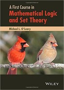
The standard interpretation of the infinity axiom is that there exists a set that contains ∅ and a ∪ {a} is an element of the set if a is an element of the set.

In Chapter 3, we noted that the elements of a set determine the set. For example, {1, 2} = {1, 2, 2}. This principle is codified by the next axiom.

AXIOM 5.1.4 [Extensionality]

Suppose A₁ and A₂ are witnesses to the empty set axiom (5.1.2). Since x ∉ A₁ and x ∉ A₂ for every x, we conclude that

Therefore, A₁ = A₂ by extensionality (Axiom 5.1.4), which means that ∅ is the witness to the empty set axiom. This uniqueness result does not appear to extend to the infinity axiom because both

and

are witnesses, provided that they are sets.

Construction Axioms

Now to build some sets. The next four axioms allow us to do this.

AXIOM 5.1.5 [Pairing]

Suppose that M and N are sets. Since {M, N} is a witness of

{M, N} is a set by the pairing axiom, and from this, we conclude that {M, {M, N}}, {N, {M, N}}, and {{M, N}} = {{M, N}, {M, N}} are sets. Because {M, M} equals {M}, pairing along with extensionality prove the existence of singletons. For example, if W is a witness to the Infinity Axiom, {∅, W}, {∅}, and {∅, {∅, W}} are sets.

AXIOM 5.1.6 [Union]

By the union axiom, M is a set, and since M ∪ N = {M, N}, we conclude that M ∪ N is a set. Furthermore, the empty set, union, and pairing axioms can be used to prove that for any n ∈ N, there exists a set of the form {a₀, a₁, ... , a_n} (Exercise 3).

AXIOM 5.1.7 [Power Set]

Because of Definition 3.3.1, the power set axiom can be written as

We conclude that for every set M, P(M) is a set by the power set axiom, and by extensionality, P(M) is the unique set of subsets of M.

The next axiom is actually what is called an axiom scheme, infinitely many axioms, one for every formula. They are sometimes called the separation axioms.

AXIOMS 5.1.8 [Subset]

For every ST-formula p(u) not containing the symbol y, the following is an axiom:

The formula p(u) in the subset axioms cannot contain the symbol y because the axioms yield the existence of this set. If y was among its symbols, the existence of y would depend on y.

The subset axioms yield many familiar sets.

• Let be a set. By a subset axiom, there exists a set C such that

  

  Observe that the symbol C does not appear in the formula

  

  Also, observe that the set C is the intersection of . Hence, is a set, and since M ∩ N = {M, N}, we conclude that M ∩ N is a set.

• By a subset axiom, there exists a set D such that

  

  so M N is a set.

Replacement Axioms

Given sets A and B, the function φ : A → B is a set because φ ⊆ A × B and A × B is a set. Suppose, instead, that the function is defined using a formula p(x, y) and that its domain is given by a set A. It cannot be concluded from Axioms 5.1.4–5.1.10 that the range {y : x ∈ A ∧ p(x, y)} is a set. However, it appears reasonable that it is. For example, define

An examination of the formula shows p(3.4, 4) and p(−7.1, −8). Since

the formula p(x, y) defines a function (Definition 4.4.10). If the domain is given to be [0, ∞), its range is the set [0, ∞) ∩ Z. Generalizing to an arbitrary p(x, y), it is expected that the range would be a set if the domain is a set. The next axiom scheme guarantees this. It was first found in correspondence between Cantor and Richard Dedekind (Cantor 1932) and Dmitry Mirimanoff (1917) with formal versions by Abraham Fraenkel (1922) and Thoralf Skolem (1922).

AXIOMS 5.1.9 [Replacement]

For every ST-formula p(t, w) not containing the symbol y, the following is an axiom:

As an example, every indexed family of sets is a set. To prove this, let I be a set and A_i be a set for all i ∈ I. Define

Observe that by E2 and E3 (Axioms 5.1.1),

Therefore, by a replacement axiom (5.1.9), there exists a set such that

so = {A_i : i ∈ I} is a set, which implies that the union and intersection of families of sets are sets.

Suppose a ∈ M and b ∈ N. By the subset and pairing axioms, we conclude that {a, b}, (a, b) = {{a}, {a, b}} (Definition 3.2.8), and {(a, b)} are sets. Therefore, fixing b,

is a family of sets, which implies that it is a set. Likewise,

is a set. Hence, by the union axiom (5.1.6),

is a set. This implies, using a subset axiom (5.1.8), that any binary relation R such that dom(R) ⊆ M and ran(R) ⊆ N is a set.

Axiom of Choice

Suppose that we are given the pairwise disjoint family of sets

It is easy to find a set S such that

Simply run through the elements of and choose an element from each set and put it in S. Since is pairwise disjoint, each choice will differ from the others. For example, it might be that

However, what happens if is an infinite set? If there was not a systematic way where elements could be chosen from the sets of , we would be left with making infinitely many choices, which is something that we cannot do. Nonetheless, it appears reasonable that there is a set S that intersects each member of exactly once. Such a set cannot be proved to exist from Axioms 5.1.2 to 5.1.9, so we need another axiom. It is called the axiom of choice. We will have to use it every time that an infinite number of arbitrary choices need to be made.

AXIOM 5.1.10 [Choice]

If is a family of pairwise disjoint, nonempty sets, there exists S ⊆ such that S ∩ A is a singleton for all A ∈ .

The statement of the axiom of choice can be written as an ST-formula (Exercise 12). Also, notice that S in Axiom 5.1.10 is a function (Exercise 13). It is called a selector.

The next follows quickly from the axiom of choice. In fact, the proposition is equivalent to the axiom (Exercise 15), so this corollary is often used as a replacement for it.

COROLLARY 5.1.11

For every binary relation R, there exists a function φ such that φ ⊆ R and dom(φ) = dom(R).

PROOF

Let R ⊆ A×B. Define = {{a}×[a]_R : a ∈ A}, which is a set by a replacement axiom (Exercise 14). Since is pairwise disjoint and the set {a} × [a]_R ≠ ∅ for all a ∈ dom(R), the axiom of choice (5.1.10) implies that there exists a selector S such that S ⊆ and S ∩ ({a} × [a]_R) is a singleton for all a ∈ dom(R). Thus, S ⊆ R, and for all a ∈ dom(R), there exists a unique b ∈ B such that a R b. This implies that S is the desired function.

Given a family of sets , define a relation R ⊆ × by

By Corollary 5.1.11, there exists a function ξ : → such that ξ(A) ∈ A for all A ∈ . The function ξ is called a choice function.

EXAMPLE 5.1.12

Let = {A_i : i ∈ I} be a family of nonempty sets. We want to define a family of singletons such that for all i ∈ I,

By Corollary 5.1.11, there exists a choice function ξ : → . The family = {{ξ(A_i)} : i ∈ I} is the desired set because ξ(A_i) ∈ A_i for all i ∈ I.

There are many theorems equivalent to the axiom of choice (5.1.10). One such result involves families of sets. Take n ∈ N and define

Observe that _n is a chain with respect to ⊆ and contains a maximal element (Definition 4.3.16), which is {0, 1, ... , n}. However, the chain

has no maximal element. There are many sets that can be added to to give it a maximal element, but the natural choice is to add the union of to the family giving

′ has a maximal element, namely, N. The generalization of this result to any family of sets was first proved by Kuratowski (1922) and then independently by Zorn (1935) for whom the theorem is named despite Kuratowski's priority. The proof given is essentially due to Zermelo (Halmos 1960).

THEOREM 5.1.13 [Zorn's Lemma]

Let be a family of sets. If ∈ for every chain of with respect to ⊆, there exists M ∈ such that M ⊄ A for all A ∈ .

PROOF

Let ξ : P() {∅} → be a choice function (Corollary 5.1.11). For every chain of , define

Notice that is the set of elements of that when added to yields a chain. Let Ch() be defined as the set of all chains of . That both and Ch() are sets is left to Exercise 17(a). Define

by

Next, suppose that ₀ is a chain of such that X(₀) = ₀. By the assumption on , we have that ₀ ∈ . To prove that ₀ is a maximal element of , take A ∈ such that ₀ ⊂ A. Since A has an element that is not in any of the elements of ₀, the union ₀ ∪ {A} is a chain properly containing ₀, which is impossible. We conclude that the theorem is proved if ₀ is shown to exist. To accomplish this, we begin with a definition. A subset of Ch() is called a tower when

Define To() to be the set of all towers of . Observe that Ch() and To() are both towers [Exercise 17(b)].

Take C ∈ To() such that C is comparable with respect to inclusion to every element of To(). Such a set C exists since ∅ is an element of To() and comparable to every element of To(). Suppose A ∈ To() such that A ⊂ C. Because To() is a tower, X(A) ∈ To(). If C ⊂ X(A), then X(A) A has at least two elements, which is impossible. Therefore,

Define

If A ⊆ C, then A ⊆ X(C) since C ⊆ X(C). Hence, every element of T is comparable to X(C). Also, T is a tower because of the following:

Hence, T = To() because T ⊆ To(). Therefore, To() is a chain because C is arbitrary [Exercise 17(c)]. Since To() is a tower,

and then

Hence, since To() is an upper bound of To(),

which yields

There are many equivalents to the axiom of choice (Rubin and Rubin 1985, Jech 1973). One of them is Zorn's lemma.

THEOREM 5.1.14

The axiom of choice is equivalent to Zorn's lemma.

PROOF

Since we have already proved that the axiom of choice (5.1.10) implies Zorn's lemma (Theorem 5.1.13), we only need to prove the converse. We must be careful to only use Axioms 5.1.2–5.1.9 and not Axiom 5.1.10.

Assume Zorn's lemma and let R be a relation. Define

Let be a chain of elements of .

We conclude that ∈ . Thus, by Zorn's lemma, there exists a maximal element Φ ∈ . This means that Φ ⊆ R and dom(Φ) ⊆ dom(R). To prove that dom(R) ⊆ dom(Φ), let (x, y) ∈ R and suppose that x ∉ dom(Φ). This implies that Φ ∪ {(x, y)} ⊆ R is a function. Hence, Φ ∪ {(x, y)} ∈ , contradicting the maximality of Φ. We conclude that Φ is the desired function, and the axiom of choice follows (Exercise 15).

There was a controversy regarding the axiom of choice when Zermelo first proposed it. Despite mathematicians having previously used it implicitly, some objected to its nonconstructive nature. The other axioms yield distinct results, but the axiom of choice results in a set with elements that are not clearly identified. Over time, however, most objections have faded. This is because the majority of mathematicians regard it as reasonable and generally those who question the axiom of choice realize that eliminating it would lead to serious problems because many proofs in various fields of mathematics rely on the axiom.

Axiom of Regularity

The ideas that led to the next axiom (also known as the axiom of foundation) can be found in Mirimanoff (1917), while the statement of the axiom is credited to Skolem (1922) and John von Neumann (1923).

AXIOM 5.1.15 [Regularity]

The main result of the regularity axiom is that it prevents sets from being elements of themselves. Suppose there exists a set A such that A ∈ A. Then, A ∩ {A} ≠ ∅, but the regularity axiom implies that A ∩ {A} should be empty.

THEOREM 5.1.16

No set is an element of itself.

If V = {x : x is a set} is a set, V ∈ V, contradicting Theorem 5.1.16. Thus, the theorem's corollary quickly follows.

COROLLARY 5.1.17

There is no set of all sets.

Because of the regularity axiom (5.1.15), A ∉ A for all sets A. Therefore, {x : x ∉ x} is not a set by, which prevents Russell's paradox from being deduced from the axioms, provided that they are consistent (Theorem 1.5.2).

The axiom of regularity is the final axiom of our chosen collection of axioms. It is believed that they do not prove any contradictions, which implies that the axioms prevent the construction of {x : x ∉ x} as a set. Therefore, we write the following definition. The collections of axioms are named after the mathematician who was primarily responsible for their selection (Zermelo 1908).

DEFINITION 5.1.18

• Axioms 5.1.2–5.1.8 are the Zermelo axioms. This collection of sentences is denoted by Z.
• Axioms 5.1.2–5.1.8 combined with replacement and regularity (Axioms 5.1.9 and 5.1.15) are the Zermelo–Fraenkel axioms, denoted by ZF.
• The Zermelo–Fraenkel axioms with the axiom of choice is denoted by ZFC.

The nonempty sets that follow from ZFC have the property that all of their elements are sets. Sets with this property are called hereditary or pure. Assuming ZFC does not prevent us from working with different types of sets, such as sets of symbols or formulas, but we must remember that such nonhereditary sets are not products of ZFC, so they must be handled with care because we do not want to fall into a paradox.

Exercises

1. Let S be a set of theory symbols. Let c₁, c₂, c₃, c₄ ∈ S be constant symbols and f ∈ S be a binary function symbol. Suppose that p(x, y) is an S-formula. Use the Equality Axioms (5.1.1) to prove the following.

(a) c₁ = c₁

(b) c₁ = c₂ ∧ c₂ = c₃ → c₁ = c₃

(c) c₁ = c₂ ∧ c₃ = c₄ → f(c₁, c₃) = f(c₂, c₄)

(d) c₁ = c₂ ∧ c₃ = c₄ → [p(f(c₁), c₃) ↔ p(f(c₂), c₄)]

2. Prove ∀x∀y(x = y → ∀u[u ∈ x ↔ u ∈ y]).

3. For any n ∈ N with n > 0, prove that there exists a set of the form {a₀, a₁, ... , a_n−1}.

4. Let be a family of sets. Prove that P( ) is a set.

5. Use a subset axiom (5.1.8) to prove that there is no set of all sets. This proves that Russell's paradox does not follow from the axiom of Z.

6. Prove that there is no set that has every singleton as an element.

7. Let A and B be sets. Define the symmetric difference of A and B by

Prove that A Δ B is a set.

8. Prove the given equations for all sets A, B, and C.

(a) A Δ ∅ = A

(b) A Δ U = Ā

(c) A Δ B = B Δ A

(d) A Δ (B Δ C) = (A Δ B) Δ C

(e) A Δ B = (A ∪ B) (B ∪ A)

(f) (A Δ B) ∩ C = (A ∩ C) Δ (B ∩ C)

9. Given sets I and A_i for all i ∈ I, show that A_i and A_i are sets.

10. Prove that A₀ × A₁ × · · · × A_n−1 is a set if A₀, A₁, ... , A_n−1 are sets.

11. Show that the Cartesian product of a nonempty family of nonempty sets is not empty.

12. Write the Axiom of Choice (5.1.10) as an ST-formula.

13. Demonstrate that a selector is a function.

14. In the proof of Corollary 5.1.11, prove that {{a} × [a]_R : a ∈ A} is a set.

15. Prove that Corollary 5.1.11 implies Axiom 5.1.10.

16. Let R = R × {0, 1}. Find a function F : R → {0, 1} such that F(a) = 0 for all a ∈ R.

17. Prove the following parts of the proof of Zorn's lemma (5.1.13).

(a) and Ch() are sets.

(b) Ch() and ∩To() are towers.

(c) To() is a chain.

18. Prove that ZF and Zorn's lemma imply the axiom of choice.

19. Use Zorn's lemma to prove that for every function φ : A → B, there exists a maximal C ⊆ A such that φ C is one-to-one.

20. Prove that if is a collection of sets such that ∈ for every chain ⊆ , then contains a maximal element.

21. Let (A, R) be a partial order. Prove that there exists an order S on A such that R ⊆ S and S is linear.

22. Use the regularity axiom (5.1.15) to prove that if {a, {a, b}} = {c, {c, d}, then a = c and b = d. This gives an alternative to Kuratowski's definition of an ordered pair (Definition 3.2.8).

23. Prove that there does not exist an infinite sequence of sets A₀, A₁, A₂, ... such that A_i+1 ∈ A_i for all i = 0, 1, 2, ... .

24. Prove that the empty set axiom (5.1.2) can be proved from the other axioms of ZFC.

25. Use Axiom 5.1.9 to prove that the subset axioms (5.1.8) can be proved from the other axioms of ZFC.

26. Let (A, R) be a poset. Prove that every chain of A is contained in a maximal chain with respect to ⊆. This is called the Hausdorff maximal princple.

27. Prove that the Hausdorff maximal principle implies Zorn's lemma, so is equivalent to the axiom of choice.

5.2 NATURAL NUMBERS

In order to study mathematics itself, as opposed to studying the contents of mathematics as when we study calculus or Euclidean geometry, we need to first develop a system in which all of mathematics can be interpreted. In such a system, we should be able to precisely define mathematical concepts, like functions and relations; construct examples of them; and write statements about them using a very precise language. ZFC with first-order logic seems like a natural choice for such an endeavor. However, in order to be a success, this system must have the ability to represent the most basic objects of mathematical study. Namely, it must be able to model numbers. Therefore, within ZFC families of sets that copy the properties of N, Z, Q, R, and C will be constructed. Since we can do this, we conclude that N, Z, Q, R, and C are themselves sets, and we also conclude that what we discover about their analogs are true about them. We begin with the natural numbers.

DEFINITION 5.2.1

For every set a, the successor of a is the set a⁺ = a ∪ {a}. If a is the successor of b, then b is the predecessor of a and we write b = a⁻.

For example, we have that {3, 5, 7}⁺ = {3, 5, 7, {3, 5, 7}} and ∅⁺ = {∅}. For convenience, write a⁺⁺ for (a⁺)⁺, so ∅⁺⁺ = {∅, {∅}}. Also, the predecessor of the set {∅, {∅}, {∅, {∅}}} is {∅, {∅}}, so write {∅, {∅}, {∅, {∅}}}⁻ = {∅, {∅}}. Furthermore, since ∅ contains no elements, we have the following.

THEOREM 5.2.2

∅ does not have a predecessor.

Although every set has a successor, we are primarily concerned with certain sets that have a particular property.

DEFINITION 5.2.3

The set A is inductive if ∅ ∈ A and a⁺ ∈ A for all a ∈ A.

Definition 5.2.3 implies that if A is inductive, A contains the sets

because

Of course, Definition 5.2.3 does not guarantee the existence of an inductive set. The infinity axiom (5.1.3) does that. Then, by a subset axiom (5.1.8),

where w is inductive can be written as

Therefore, the collection that contains the elements that are common to all inductive sets is a set, and we can make the next definition (von Neumann 1923).

DEFINITION 5.2.4

An element that is a member of every inductive set is called a natural number. Let ω denote the set of natural numbers. That is,

Definition 5.2.4 suggests that the elements of ω will be interpreted to represent the elements of N, so represent each natural number with the appropriate element of N:

Although the choice of which sets should represent the numbers of N is arbitrary, our choice does have some fortunate properties. For example, the number of elements in each natural number and the number of N that it represents are the same. Moreover, notice that each natural number can be written as

and also note that

The empty set is an element of ω by definition, so suppose n ∈ ω and take A to be an inductive set. Since n is a natural number, n ∈ A, and since A is inductive, n⁺ ∈ A. Because A is arbitrary, we conclude that n⁺ is an element of every inductive set, so n⁺ ∈ ω (Definition 5.2.4). This proves the next theorem.

THEOREM 5.2.5

ω is inductive.

The proof of the next theorem is left to Exercise 5.

THEOREM 5.2.6

If A is an inductive set and A ⊆ ω, then A = ω.

Order

Because we want to interpret ω so that it represents N, we should be able to order ω as N is ordered by ≤. That is, we need to find a partial order on ω that is also a well-order. To do this, we start with a definition.

DEFINITION 5.2.7

A set A is transitive means for all a and b, if b ∈ a and a ∈ A, then b ∈ A.

Observe that ∅ is transitive because a ∈ ∅ is always false. More transitive sets are found in the next theorem.

THEOREM 5.2.8

• Every natural number is transitive.
• ω is transitive.

PROOF

The proof of the second part is left to Exercise 4. We prove the first by defining

We have already noted that 0 ∈ A, so assume that n ∈ A and let b ∈ a and a ∈ n ∪ {n}. If a ∈ {n}, then b ∈ n. If a ∈ n, then by hypothesis, b ∈ n. In either case, b ∈ n⁺ since n ⊆ n⁺, so n⁺ ∈ A. Hence, A is inductive, so A = ω by Theorem 5.2.6.

In addition to being transitive, each element of ω has another useful property that provides another reason why their choice was a wise one.

LEMMA 5.2.9

If m, n ∈ ω, then m ⊂ n if and only if m ∈ n.

PROOF

Take m, n ∈ ω. If m ∈ n, then m ⊂ n since n is transitive (Exercise 3). To prove the converse, define

We show that A is inductive. Trivially, 0 ∈ A. Now take n ∈ A and let m ∈ ω such that m ⊂ n⁺. We have two cases to consider.

For example, we see that 2 ∈ 3 and 2 ⊂ 3 because

and

Now use Lemma 5.2.9 to define an order on ω. Instead of using , we use ≤ to copy the order on N.

DEFINITION 5.2.10

For all m, n ∈ ω, let

Define m < n to mean m ≤ n but m ≠ n.

Lemma 5.2.9 in conjunction with Definition 5.2.10 implies that for all m, n ∈ ω we have that

The order of Definition 5.2.10 makes ω a chain with ∅ as its least element.

THEOREM 5.2.11

(ω, ≤) is a linear order.

PROOF

That (ω, ≤) is a poset follows as in Example 4.3.9. To show that ω is a chain under ≤, define

We prove that A is inductive.

We can now quickly prove the following.

COROLLARY 5.2.12

For all m, n ∈ ω, if m⁺ = n⁺, then m = n.

PROOF

Let m and n be natural numbers and assume that

Take x ∈ m. Then, x ∈ n or x = n. If x ∈ n, then m ⊆ n, so suppose that x = n. This implies that n ∈ m, so m ≠ n by Theorem 5.1.16. However, we then have m ∈ n by (5.3), which contradicts the trichotomy law (Theorem 4.3.21). Similarly, we can prove that n ⊆ m.

Since the successor defines a function S : ω → ω where S(n) = n⁺, Corollary 5.2.12 implies that S is one-to-one.

Thereom 5.2.11 shows that (ω, ≤) is a linear order as (N, ≤) is a linear order. The next theorem shows that the similarity goes further.

THEOREM 5.2.13

(ω, ≤) is a well-ordered set.

PROOF

By Theorem 5.2.11, (ω, ≤) is a linear order. To prove that it is well-ordered, suppose that A ⊆ ω such that A does not have a least element. Define

We prove that B is inductive.

Therefore, B = ω, which implies that A is empty.

Recursion

The familiar factorial is defined recursively as

A recursive definition is one that is given in terms of itself. This is illustrated in (5.5) where the factorial is defined using the factorial. It appears that the factorial is a function N → N, but a function is a set, so why do (5.4) and (5.5) define a set? Such a definition is not found among the axioms of Section 5.1 or the methods of Section 3.1. That they do define a function requires an important theorem.

THEOREM 5.2.14 [Recursion]

Let A be a set and a ∈ A. If g is a function A → A, there exists a unique function f : ω → A such that

PROOF

Let g : A → A be a function. Define

Note that is a set by a subset axiom (5.1.8) and is nonempty because ω×A ∈ . Let

Observe that f ∈ (Exercise 8). Define

We prove that D is inductive.

Hence, f is a function ω → A (Theorem 5.2.6). We confirm that f has the desired properties.

To prove that f is unique, let f′ : ω → A be a function such that f′(0) = a and f′(n⁺) = g(f′(n)) for all n ∈ ω. Let

The set E is inductive because f(0) = a = f′(0) and assuming n ∈ ω we have that f(n⁺) = g(f(n)) = g(f′(n)) = f′(n⁺).

The factorial function has domain N but the recursion theorem (5.2.14) gives a function with domain ω and uses the successor of Definition 5.2.1. We need a connection between N and ω. We do this by defining two operations on ω that we designate by + and · and then showing that the basic properties of ω under these two operations are the same as the basic properties of N under standard addition and multiplication.

Arithmetic

We begin with addition. Let g : ω → ω be defined by g(n) = n⁺. For every m ∈ ω, by Theorem 5.2.14, there exists a unique function f_m : ω → ω such that

and for all n ∈ ω,

Define

Since f_m is a function for every n ∈ ω, the set a is a binary operation (Definition 4.4.26). Observe that for all m, n ∈ ω,

• a(m, 0) = m,
• a(m, n⁺) = a(m, n)⁺.

We know that for every k, l ∈ N, we have that k + 0 = k and to add k + l, one simply adds 1 a total of l times to k. This is essentially what a does to the natural numbers. For example, for 1, 3, 4 ∈ N,

and for 1, 2, 3, 4 ∈ ω (page 238),

Therefore, we choose a to be addition on ω. To define the addition, we only need to cite the two properties given in Theorem 5.2.14. Since each f_m is unique, there is no other function to which the definition could be referring. Therefore, we can define addition recursively.

DEFINITION 5.2.15

For all m, n ∈ ω,

Notice that m⁺ = (m + 0)⁺ = m + 0⁺ = m + 1. Furthermore, using the notation from page 238, we conclude that 1 + 3 = 4 because a(1, 3) = 4.

The following lemma shows that the addition given in Definition 5.2.15 has a property similar to that of commutativity.

LEMMA 5.2.16

For all m, n ∈ ω,

PROOF

Let m, n ∈ ω. To prove that 0 + n = n, we show that

is inductive.

To prove that m⁺ + n = (m + n)⁺, we show that

is inductive.

Now to see that + behaves on ω as + behaves on N, we use Definition 4.4.31.

THEOREM 5.2.17

• The binary operation + on ω is associative and commutative.
• 0 is the additive identity for ω.

PROOF

0 is the additive identity by Definition 5.2.15 and Lemma 5.2.16, and that + is associative on ω is Exercise 14. To show that + is commutative, let m ∈ ω and define

As has been our strategy, we show that A is inductive.

Multiplication on N can be viewed as iterated addition. For example,

so we define multiplication recursively along these lines. As with addition, the result is a binary operation by Theorem 5.2.14.

DEFINITION 5.2.18

For all m, n ∈ ω,

For example, 3 · 4 = 12 because

where ([3 + 3] + 3) + 3 = 12 is left to Exercise 13.

The next result is analogous to Lemma 5.2.16. Its proof is left to Exercise 9.

LEMMA 5.2.19

For all m, n ∈ m,

We now prove that · on ω behaves as · on N and that + and · on ω interact with each other via the distributive law as the two operations on N. For the proof, we introduce two common conventions for these two operations.

• So that we lessen the use of parentheses, define · to have precedence over +, and read from left to right. That is,

  

  and

  

• Define mn = m · n.

THEOREM 5.2.20

• The binary operation · on ω is associative and commutative.
• 1 is the multiplicative identity for ω.
• The distributive law holds for ω. This means that for all m, n, o ∈ ω,

  

PROOF

That the associative and commutative properties hold is Exercise 12. To prove the other parts of the theorem, let m, n, o ∈ ω. Since 0⁺ = 1, by Definition 5.2.18 and Lemma 5.2.16,

and by Lemma 5.2.19 and Definition 5.2.15, we have that 1m = m. To show that the distributive law holds, define

Since 0(n + o) = 0 and 0n + 0o = 0 + 0 = 0, we have that 0 ∈ A. Now suppose that m ∈ A. That is,

Therefore, m⁺ ∈ A because

EXAMPLE 5.2.21

We revisit the factorial function. Since addition and multiplication are now defined on ω, let g : ω × ω → ω × ω be the function

Theorem 5.2.14 implies that there exists a unique function f : ω → ω × ω such that

and

Let π be the projection map π(k, l) = l. By Theorem 5.2.6 and Exercise 10, we conclude that for all n ∈ ω,

Therefore, the factorial function n!, which is defined recursively by

is π f by the uniqueness of f.

To solve an equation like 6 + 2x = 14 where the coefficients are from N, we can use the cancellation law and write

For equations with coefficients in ω, we need a similar law.

THEOREM 5.2.22 [Cancellation]

Let a, b, c ∈ ω.

PROOF

The proof for multiplication is Exercise 15. For addition, define

Clearly, 0 ∈ A, so assume n ∈ A. To prove that n⁺ ∈ A, let b, c ∈ ω and suppose that n⁺ + b = n⁺ + c. Then, (n + b)⁺ = (n + c)⁺ by Lemma 5.2.16, so n + b = n + c by Corollary 5.2.12. Hence, b = c because n ∈ A.

Exercises

1. For every set A, show that A⁺ is a set.

2. For every n ∈ ω, show that n⁺⁺⁺⁺⁺ = n + 5.

3. Show that the following are equivalent.

• A is transitive.
• If a ∈ A, then a ⊂ A.
• A ⊆ P(A).
• A ⊆ A.
• (A⁺) = A.

4. Prove that ω is transitive.

5. Prove Theorem 5.2.6.

6. Let A ⊆ ω. Show that if A = A, then A = ω.

7. Take u, v, x, y ∈ ω and assume that u + x = v + y. Prove that u ∈ v if and only if y ∈ x.

8. Prove that f ∈ in the proof of Theorem 5.2.14.

9. Prove Lemma 5.2.19.

10. Prove (5.7) from Example 5.2.21.

11. Let A be a set and φ : A → A be a one-to-one function. Take a ∈ A ran(φ). Recursively define f : ω → A such that

Prove that f is one-to-one.

12. Let m, n, o ∈ m. Prove the given equations.

(a) mn = nm.

(b) m(n + o) = mn + mo.

13. Show that ([3 + 3] + 3) + 3 = 12.

14. Prove that addition on ω is associative.

15. For all a, b, c ∈ ω with a ≠ 0, prove that if ab = ac, then b = c.

16. Show that for all m, n ∈ ω, if mn = 0, then m = 0 or n = 0.

17. We define exponentiation on ω. For all n ∈ ω,

(a) Use the recursion (Theorem 5.2.14) to prove that this defines a function ω × ω → ω.

(b) Show that exponentiation on ω is one-to-one.

18. Let x, y, x ∈ ω. Use the definition of Exercise 17 to prove the given equations.

(a) x^y+z = x^yx^z.

(b) (xy)^z = x^zy^z.

(c) (x^y)^z = x^yz.

19. Let m, n, k ∈ ω. Assume that m ≤ n and 0 ≤ k. Demonstrate the following.

(a) m + k ≤ n + k.

(b) mk ≤ nk.

(c) m^k ≤ n^k.

5.3 INTEGERS AND RATIONAL NUMBERS

Now that we have defined within set theory the set of natural numbers and confirmed its basic properties, we wish to continue this with other sets of numbers. We begin with the integers.

Integers

We build the integers using the natural numbers. The problem is how to define the negative integers. We need to decide how to represent the adjoining of the negative sign to a natural number. One option that might work is to use ordered pairs. These are always good options when extra information needs to be included with each element of a set. For example, (4, 0) could represent 4 because 4 − 0 = 4, and (0, 4) could represent −4 because 0 − 4 = −4. However, this is a problem because we did not define subtraction on ω, so we need another solution. Our decision is to generalize this idea of subtracting coordinates to the set ω × ω, but use addition to do it. Since there are infinitely many pairs (m, n) such that m − n = 4, we equate them by using the equivalence relation of Exercise 4.2.2.

DEFINITION 5.3.1

Let R be the equivalence relation on ω × ω defined by

Define = (ω × ω)/R to be the set of integers.

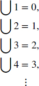
Using Definition 5.3.1 we associate elements of Z with elements of :

Notice that because 0 and 2 are elements of ω, the equivalence class [(0, 2)] is the name for [(∅, {∅, {∅}})]. Also,

The ordering of is defined in terms of the ordering on ω. Be careful to note that the symbol ≤ will represent two different orders, one on and one on ω (Definition 5.2.10). This overuse of the symbol will not lead to confusion because the order will be clear from context. For example, in the next definition, the first ≤ is the order on , and the second ≤ is the order on ω.

DEFINITION 5.3.2

For all [(m, n)], [(m′, n′)] ∈ , define

and

Since −4 = [(0, 4)] and 3 = [(5, 2)], we have that −4 < 3 because 0 + 2 < 5 + 4.

Since (, ≤) has no least element (Exercise 3), it is not well-ordered. However, it is a chain. Note that in the proof the symbol ≤ is again overused.

THEOREM 5.3.3

(, ≤) is a linear order.

PROOF

We use the fact that the order on ω is a linear order (Theorem 5.2.11). Let a, b ∈ , so a = (m, n) and b = (m′, n′) for some m, n, m′, n′ ∈ ω.

Although ω is not a subset of like N is a subset of Z, the set ω can be embedded in (Definition 4.5.29). This is shown by the function φ : ω → defined by

We see that φ is one-to-one because [(m, 0)] = [(n, 0)] implies that m = n. The function φ is then an order isomorphism using the relation from Definition 5.3.2 (Exercise 1).

As with ω, we define what it means to add and multiply two integers.

DEFINITION 5.3.4

Let [(m, n)], [(u, v)] ∈ .

For example, the equation in ,

corresponds to the equation in Z,

and the equation

corresponds to the equation

Before we check the properties of + and · on , we should confirm that these are well-defined. Exercise 5 is for addition. To prove that multiplication is well-defined, let [(m, n)] = [(m′, n′)] and [(u, v)] = [(u′, v′)]. Then, m + n′ = m′ + n and u + v′ = u′ + v. Hence, by Theorem 5.2.20 in ω we have that

Therefore,

equals

so by Cancellation (Theorem 5.2.22),

This implies by Definition 5.3.1 that

and this by Definition 5.3.4 implies that

We follow the same order of operations with + and · on as on ω and also write mn for m · n.

THEOREM 5.3.5

• The binary operations + and · on are associative and commutative.
• [(0, 0)] is the additive identity for , and [(1, 0)] is its multiplicative identity.
• For every a ∈ , there exists an additive inverse of a.
• For all a, b, c ∈ , the distributive law holds.

PROOF

We will prove parts of the first and third properties and leave the remaining properties to Exercise 6. Let a, b, c ∈ . This means that there exist natural numbers m, n, r, s, u, and v such that a = [(m, n)], b = [(r, s)], and c = [(u, v)]. Then,

and

To prove that every element of has an additive inverse, notice that

Therefore, if a = [(m, n)], the additive inverse of a is [(n, m)].

For all n ∈ , denote the additive inverse of n by −n, and for all m, n, r, s ∈ ω, define

Rational Numbers

As the integers were built using ω, so the set of rational numbers will be built using . Its definition is motivated by the behavior of fractions in Q. For instance,

because 2 · 12 = 3 · 8. Imagining that the ordered pair (m, n) represents the fraction m/n, we define an equivalence relation. Notice that this is essentially the relation from Example 4.2.5. Notice that is defined using addition (Definition 5.3.1) while the rational numbers are defined using multiplication.

DEFINITION 5.3.6

Let S be the equivalence relation on × ( {0}) defined by

Define = [ × ( {0})]/S to be the set of rational numbers.

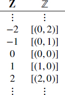
Using Definition 5.3.6, we associate elements of Q with elements of :

Notice that since 1, 2 ∈ , the equivalence class [(1, 2)] is the name for

where R is the relation of Definition 5.3.1. Also,

We next define a partial order on .

DEFINITION 5.3.7

For all [(m, n)], [(m′, n′)] ∈ , define

and

When working with , we often denote [(m, n)] by m/n or and [(m, 1)] by m. Thus, since 2/3 = [(2, 3)] and 7/8 = [(7, 8)], we conclude that 2/3 < 7/8 because 2·8 < 3·7.

As ω can be embedded in , so can be embedded in . The function that can be used is

defined by

(See Exercise 2) Using the function φ (5.8), we see that ω can be embedded in via the order isomorphism ψ φ.

Since (, ≤) has no least element (Exercise 3), it is not well-ordered. However, it is a chain (Exercise 11).

THEOREM 5.3.8

(, ≤) is a linear order.

Lastly, we define two operations on that represent the standard operations of + and · on Q.

DEFINITION 5.3.9

Let [(m, n)], [(m′, n′)] ∈ .

That + and · as given in Definition 5.3.9 are binary operations is left to Exercise 13.

As examples of these two operations, the equation in

corresponds to the equation in Q

and the equation in

corresponds to the equation in Q

We follow the same order of operations with + and · on as on and also write mn for m · n.

THEOREM 5.3.10

• The binary operations + and · on are associative and commutative.
• [(0, 1)] is the additive identity, and [(1, 1)] is the multiplicative identity.
• Every rational number has an additive inverse, and every element of {[(0, 1)]} has a multiplicative inverse.
• The distributive law holds.

PROOF

Since [(m, n)] · [(1, 1)] = [(m · 1, n · 1)] = [(m, n)] for all [(m, n)] ∈ and multiplication is commutative, the multiplicative identity of is [(1, 1)]. Also, because m ≠ 0 and n ≠ 0 implies that

every element of [(0, 1)] has a multiplicative inverse. The other properties are left to Exercise 14.

For all a, b ∈ with b ≠ 0, denote the additive inverse of a by −a and the multiplicative inverse of b by b⁻¹.

Actual Numbers

We now use the elements of ω, , and as if they were the actual elements of N, Z, and Q. For example, we understand the formula n ∈ to mean that n is an integer of Definition 5.3.1 with all of the properties of n ∈ Z. Also, when we write that the formula p(n) is satisfied by some rational number a, we interpret this to mean that p(a) with a ∈ where a has all of the properties of a ∈ Q. This allows us to use the set properties of a natural number, integer, or rational number when needed yet also use the results we know concerning the actual numbers. That the partial orders and binary operations defined on ω, , and have essentially the same properties as those on N, Z, and Q allows for this association of properties to be legitimate.

Exercises

1. Prove that the function φ (5.8) is an order isomorphism using the order of Definition 5.3.2.

2. Prove that the function ψ (5.9) is an order isomorphism using the order of Definition 5.3.7.

3. Show that (, ≤) and (, ≤) do not have least elements.

4. Prove that ≤ is transitive on .

5. Prove that + is well-defined on .

6. Complete the remaining proofs of the properties of Theorem 5.3.5.

7. Show that every nonempty subset of ⁻ = {n : n ∈ ∧ n < 0} has a greatest element.

8. Let m, n ∈ and k ∈ ⁻ (Exercise 7) Prove that if m ≤ n, then nk ≤ mk.

9. Prove that for every m, n ∈ , if mn = 0, then m = 0 or n = 0. Show that this same result also holds for .

10. The cancellation law for the integers states that for all m, n, k ∈ ,

• if m + k = n + k, then m = n,
• if mk = nk and k ≠ 0, then m = n.

Prove that the cancellation law holds for . Prove that a similar law holds for .

11. Prove that (, ≤) is a chain.

12. Demonstrate that every nonempty set of integers with a lower bound with respect to ≤ has a least element.

13. Show that + and · as given in Definition 5.3.9 are binary operations on .

14. Prove the remaining parts of Theorem 5.3.10.

15. Let a, b, c, d ∈ . Prove.

(a) If 0 ≤ a ≤ c and 0 ≤ b ≤ d, then ab ≤ cd.

(b) If 0 ≤ a < c and 0 ≤ b < d, then ab < cd.

16. Let a, b ∈ . Prove that if b < 0, then a + b < a.

17. Let a, b ∈ . Prove that if a ≥ 0 and b < 1, then ab ≤ a.

18. Prove that between any two rational numbers is a rational number. This means that is dense. Show that this is not the case for .

19. Generalize the definition of exponentiation given in Exercise 5.2.17 to . Prove that this defines a one-to-one function × (⁺ ∪ {0}) → . Does the proof require recursion (Theorem 5.2.14)?

20. Let m, n, k ∈ . Assume that m ≤ n. Demonstrate the following.

(a) m + k ≤ n + k.

(b) mk ≤ nk if 0 ≤ k.

(c) nk ≤ mk if k < 0.

(d) m^k ≤ n^k if k ≥ 0.

21. Let φ : ω → be the embedding defined by (5.8). Define f : ω × ω → ω by f(m, n) = mⁿ and g : × (⁺ ∪ {0}) → by g(u, v) = u^v. Prove that for all m, n ∈ ω, we have that g(φ(m), φ(n)) = φ(f(m, n)). Explain the significance of this result.

5.4 MATHEMATICAL INDUCTION

Suppose that we want to prove p(n) for all integers n greater than or equal to some n₀. Our previous method (Section 2.4) is to take an arbitrary n ≥ n₀ and try to prove p(n). If this is not possible, we might be tempted to try proving p(n) for each n individually. This is impossible because it would take infinitely many steps. Instead, we combine the results of Sections 5.2 and 5.3 and use the next theorem.

THEOREM 5.4.1 [Mathematical Induction 1]

Let p(k) be a formula. For any n₀ ∈ , if

then

PROOF

Assume p(n₀) and that p(k) implies p(k + 1) for all integers k ≥ n₀. Define

Notice that 0 ∈ A ⇔ p(n₀), 1 ∈ A ⇔ p(n₀ + 1), and so on. To prove p(k) for all integers k ≥ n₀, we show that A is inductive.

Theorem 5.4.1 gives rise to a standard proof technique known as mathematical induction. First, prove p(n₀). Then, show that p(n) implies p(n + 1) for every integer n ≥ n₀. Often an analogy of dominoes is used to explain this. Proving p(n₀) is like tipping over the first domino, and then proving the implication shows that the dominoes have been set properly. This means that by modus ponens, if p(n₀ + 1) is true, then p(n₀ + 2) is true, and so forth, each falling like dominoes:

This two-step process is characteristic of proofs by mathematical induction. So much so, the two stages have their own terminology.

• Proving p(n₀) is called the basis case. It is typically the easiest part of the proof but should, nonetheless, be explicitly shown.
• Proving that p(n) implies p(n + 1) is the induction step. For this, we typically use direct proof, assuming p(n) to show p(n + 1). The assumption is called the induction hypothesis.

Often induction is performed to prove a formula for all positive integers, so to represent this set, define

EXAMPLE 5.4.2

Prove p(k) for all k ∈ ⁺, where

Proceed by mathematical induction.

EXAMPLE 5.4.3

Let x be a positive rational number. To prove that for any k ∈ ⁺,

we proceed by mathematical induction.

EXAMPLE 5.4.4

Recursively define a sequence of numbers,

The sequence is

and we conjecture that a_k = 3 · 2^k–1 for all positive integers k. We prove this by mathematical induction.

• For the basis case, a₁ = 3 · 2⁰ = 3.
• Let n > 1 and assume a_n = 3 · 2ⁿ⁻¹. Then,

  

EXAMPLE 5.4.5

Use mathematical induction to prove that k³ < k! for all integers, k ≥ 6.

Combinatorics

We now use mathematical induction to prove some basic results from two areas of mathematics. The first is combinatorics, the study of the properties that sets have based purely on their size.

A permutation of a given set is an arrangement of the elements of the set. For example, the number of permutations of {a, b, c, d, e, f} is 720. If we were to write all of the permutations in a list, it would look like the following:

We observe that 6! = 720 and hypothesize that the number of permutations of a set with k elements is k!. To prove it, we use mathematical induction.

• There is only one way to write the elements of a singleton. Since 1! = 1, we have proved the basis case.
• Assume that the number of permutations of a set with n ≥ 1 elements is n!. Let A = {a₁, a₂, ... , a_n+1} be a set with n + 1 elements. By induction, there are n! permutations of the set {a₁, a₂, ... , a_n}. After writing the permutations in a list, notice that there are n + 1 columns before, between, and after each element of the permutations:

  

  To form the permutations of A, place a_n+1 into the positions of each empty column. For example, if a_n+1 is put into the first column, the following permutations are obtained:

  

  Since there are n! rows with n + 1 ways to add a_n+1 to each row, we conclude that there are (n + 1)n! = (n + 1)! permutations of A.

This argument proves the first theorem.

THEOREM 5.4.6

Let n ∈ ⁺. The number of permutations of a set with n elements is n!.

Suppose that we do not want to rearrange the entire set but only subsets of it. For example, let A = {a, b, c, d, e}. To see all three-element permutations of A, look at the following list:

There are 60 arrangements because there are 5 choices for the first entry. Once that is chosen, there are only 4 left for the second, and then 3 for the last. We calculate that as

Generalizing, we define for all n, r ∈ ω,

and we conclude the following theorem.

THEOREM 5.4.7

Let r, n ∈ ⁺. The number of permutations of r elements from a set with n elements is _nP_r.

Now suppose that we only want to count subsets. For example, A = {a, b, c, d, e} has 10 subsets of three elements. They are the following:

The number of subsets can be calculated by considering the next grid.

There are ₅P₃ permutations with three elements from A. They are found as the entries in the grid. However, since we are looking at subsets, we do not want to count abc as different from acb because {a, b, c} = {a, c, b}. For this reason, all elements in any given row of the grid are considered as one subset. Each row has 6 = 3! entries because that is the number of permutations of a set with three elements. Hence, multiplying the number of rows by the number of columns gives

Therefore,

A generalization of this calculation leads to the formula for the arbitrary binomial coefficient,

where n, r ∈ ω. Read as “n choose r.” A generalization of the argument leads to the next theorem.

THEOREM 5.4.8

Let n, r ∈ ⁺. The number of subsets of r elements from a set with n elements is .

When we expand (x + 1)³, we find that

To prove this for any binomial (x + y)ⁿ, we need the following equation. It was proved by Blaise Pascal (1653). The proof is Exercise 7.

LEMMA 5.4.9 [Pascal's Identity]

If n, r ∈ ω so that n ≥ r,

THEOREM 5.4.10 [Binomial Theorem]

Let n ∈ ⁺. Then,

PROOF

• Since ,

  

• Assume for k ∈ ⁺,

  

  Then,

  

  Multiplying the (x + y) term through the summation yields

  

  Taking out the (k + 1)-degree terms and shifting the index on the second summation gives

  

  which using Pascal's identity (Lemma 5.4.9) equals

  

  and this is

  

Euclid's Lemma

Our second application of mathematical induction comes from number theory. It is the study of the greatest common divisor (Definition 3.3.11). We begin with a lemma.

LEMMA 5.4.11

Let a, b, c ∈ such that a ≠ 0 or b ≠ 0. If a | bc and gcd(a, b) = 1, then a | c.

PROOF

Assume a | bc and gcd(a, b) = 1. Then, bc = ak for some k ∈ . By Theorem 4.3.32, there exist m, n ∈ such that

Therefore, a | c because

Suppose that p ∈ is a prime (Example 2.4.18) that does not divide a. We show that gcd(a, p) = 1. Take d > 0 and assume d | a and d | p. Since p is prime, d = 1 or d = p. Since p a, we conclude that d must equal 1, which means gcd(a, p) = 1. Use this to prove the next result attributed to Euclid (Elements VII.30).

THEOREM 5.4.12 [Euclid's Lemma]

An integer p > 1 is prime if and only if p | ab implies p | a or p | b for all a, b ∈ .

PROOF

• Let p be prime. Suppose p | ab but p a. Then, gcd(a, p) = 1. Therefore, p | b by Theorem 5.4.11.
• Let p > 1. Suppose p satisfies the condition,

  

  Assume p is not prime. This means that there are integers c and d so that p = cd with 1 < c ≤ d < p. Hence, p | cd. By hypothesis, p | c or p | d. However, since c, d < p, p can divide neither c nor d. This is a contradiction. Hence, p must be prime.

Since 6 divides 3 · 4 but 6 3 and 6 4, the lemma tells us that 6 is not prime. On the other hand, if p is a prime that divides 12, then p divides 4 or 3. This means that p = 2 or p = 3.

The next theorem is a generalization of Euclid's lemma. Its proof uses mathematical induction.

THEOREM 5.4.13

Let p be prime and a_i ∈ for i = 0, 1, ... , n − 1. If p | a₀a₁ · · · a_n−1, then p | a_j for some j = 0, 1, ... , n − 1.

PROOF

• The case when n = 1 is trivial because p divides a₀ by definition of the product.
• Assume if p | a₀a₁ · · · a_n−1, then p | a_j for some j = 0, 1, ... , n − 1. Suppose p | a₀a₁ · · · a_n. Then, by Lemma 5.4.12,

  

  If p | a_n, we are done. Otherwise, p divides a₀a₁ · · · a_n−1. Hence, p divides one of the a_i by induction.

Exercises

1. Let n ∈ ⁺. Prove.

2. Prove for all positive integers n.

3. Let n ∈ ⁺. Prove.

4. Let n ∈ . Prove.

(a) n² < 2ⁿ for all n ≥ 5.

(b) ²n < n! for all n ≥ 4.

(c) n² < n! for all n ≥ 4.

5. For n ∈ ⁺, prove that if A has n elements, P(A) has 2ⁿ elements.

6. Prove that the number of lines in a truth table with n propositional variables is 2ⁿ.

7. Demonstrate Pascal's identity (Lemma 5.4.9).

8. For all integers n ≥ r ≥ 0, prove the given equations.

9. Let n, r ∈ ⁺ with n ≥ r. Prove.

10. Let n ≥ 2 be an integer and prove the given equations.

11. Let n and r be positive integers and n ≥ r. Use induction to show the given equations.

12. Prove the following for all n ∈ ω.

(a) 5 | n⁵ − n

(b) 9 | n³ + (n + 1)³ + (n + 2)³

(c) 8 | 5²ⁿ + 7

(d) 5 | 3³ⁿ⁺¹ + 2ⁿ⁺¹

13. If p is prime and a and b are positive integers such that a + b = p, prove that gcd(a, b) = 1.

14. Prove for all n ∈ ⁺, there exist n consecutive composite integers (Example 2.4.18) by showing that (n +1)! +2, (n + 1)! + 3, ... , (n + 1)! + n + 1 are composite.

15. Prove.

(a) If a ≠ 0, then a · gcd(b, c) = gcd(ab, ac).

(b) Prove if gcd(a_i, b) = 1 for i = 1, . . ., n, then gcd(a₁ · a₂ · · · a_n, b) = 1).

16. For k ∈ ⁺, let a₀, a₁, . . ., a_k−1 ∈ ω, not all equal to zero. Define

to mean that g is the greatest integer such that g | a_i for all i = 0, 1, ... , k − 1. Assuming k ≥ 3, prove the given equations.

(a) gcd(a₀, a₁, ... , a_k−1) = gcd(a₀, a₁, ... , a_k−3, gcd(a_k−2, a_k−1))

(b) gcd(ca₀, ca₁, ... , ca_k−1) = c gcd(a₀, a₁, ... , a_k−1) for all integers c ≠ 0

5.5 STRONG INDUCTION

Suppose we want to find an equation for the terms of a sequence defined recursively in which each term is based on two or more previous terms. To prove that such an equation is correct, we modify mathematical induction. Remember the domino picture that we used to explain how mathematical induction works (page 258). The first domino is tipped causing the second to fall, which in turn causes the third to fall. By the time the sequence of falls reaches the n + 1 domino, n dominoes have fallen. This means that sentences p(1) through p(n) have been proved true. It is at this point that p(n + 1) is proved. This is the intuition behind the next theorem. It is sometimes called strong induction.

THEOREM 5.5.1 [Mathematical Induction 2]

Let p(k) be a formula. For any n₀ ∈ , if

then

PROOF

Assume p(n₀) and

for k ∈ ω. Define

We proceed with the induction.

Therefore, q(n) is true for all n ∈ ω (Theorem 5.4.1). Hence, p(n) for all integers n ≥ n₀.

Fibonacci Sequence

Leonardo of Pisa (known as Fibonacci) in his 1202 work Liber abaci posed a problem about how a certain population of rabbits increases with time (Fibonacci and Sigler 2002). Each rabbit that is at least 2 months old is considered an adult. It is a young rabbit if it is a month old. Otherwise, it is a baby. The rules that govern the population are as follows:

• No rabbits die.
• The population starts with a pair of adult rabbits.
• Each pair of adult rabbits will bear a new pair each month.

The population then grows according to the following table:

It appears that the number of adult (or baby) pairs at month n is given by the sequence,

This is known as the Fibonacci sequence, and each term of the sequence is called a Fibonacci number. Let F_n denote the nth term of the sequence. So

Each term of the sequence can be calculated recursively by

Since we have only checked a few terms, we have not proved that F_n is equal to the number of adult pairs in the nth month. To show this, we use strong induction. Since the recursive definition starts by explicitly defining F₁ and F₂, the basis case for the induction will prove that the formula holds for n = 1 and n = 2.

• From the table, in each of the first 2 months, there is exactly one adult pair of rabbits. This coincides with F₁ = 1 and F₂ = 1 in (5.12).
• Let n > 2, and assume that F_k equals the number of adult pairs in the kth month for all k ≤ n. Because of the third rule, the number of pairs of adults in any month is the same as the number of adult pairs in the previous month plus the number of baby pairs 2 months prior. Therefore,

  

It turns out that the Fibonacci sequence is closely related to another famous object of study in the history of mathematics. Letting n ≥ 1, define

The first seven terms of this sequence are

This sequence has a limit that we call τ. To find this limit, notice that

Because a_n−1 = F_n/F_n−1 when n > 1,

and therefore,

Because

we conclude that

Therefore, are the solutions to (5.13), but since F_n+1/F_n > 0, we take the positive value and find that

The number τ is called the golden ratio. It was considered by the ancient Greeks to represent the ratio of the sides of the most beautiful rectangle.

EXAMPLE 5.5.2

Prove F_n ≤ τⁿ⁻¹ when n ≥ 2 using strong induction.

Unique Factorization

Theorem 5.4.13 states that if a prime divides an integer, it divides one of the factors of the integer. It appears reasonable that any integer can then be written as a product that includes all of its prime divisors. For example, we can write 126 = 2 · 3 · 3 · 7, and this is essentially the only way in which we can write 126 as a product of primes. All of this is summarized in the next theorem. It is also known as the fundamental theorem of arithmetic. It is the reason the primes are important. They are the building blocks of the integers.

THEOREM 5.5.3 [Unique Factorization]

If n > 1, there exists a unique sequence of primes p₀ ≤ p₁ ≤ · · · ≤ p_k (k ∈ ω) such that n = p₀p₁ · · · p_k.

PROOF

Prove existence with strong induction on n.

For uniqueness, suppose that there are two sets of primes

so that

By canceling, if necessary, we can assume the sides have no common primes. If the cancellation yields 1 = 1, the sets of primes are the same. In order to obtain a contradiction, assume that there is at least one prime remaining on the left-hand side. Suppose it is p₀. If the product on the right equals 1, then p₀ | 1, which is impossible. If there are primes remaining on the right, p₀ divides one of them by Lemma 5.4.12. This is also a contradiction, since the sides have no common prime factors because of the cancellation. Hence, the two sequences must be the same.

Unique Factorization allows us to make the following definition.

DEFINITION 5.5.4

Let n ∈ ⁺. If p₀, p₁, ... , p_k−1 are distinct primes and r₀, r₁, ... , r_k−1 are natural numbers such that

then is called a prime power decomposition of n.

EXAMPLE 5.5.5

Consider the integer 360. It has 2³ · 3² · 5¹ as a prime power decomposition. If the exponents are limited to positive integers, the expression is unique. In this sense, we can say that 2³ · 3² · 5¹ is the prime power decomposition of 360. However, there are times when primes need to be included in the product that are not factors of the integer. By setting the exponent to zero, these primes can be included. For example, we can also write 360 as 2³ · 3² · 5¹ · 7⁰.

EXAMPLE 5.5.6

Suppose n ∈ such that n > 1. Use unique factorization (Theorem 5.5.3) to prove that n is a perfect square if and only if all powers in a prime power decomposition of n are even.

Exercises

1. Given each recursive definition, prove the formula for a_n holds for all positive integers n.

(a) If a₁ = −1 and a_n = −a_n−1, then a_n = (−1)ⁿ.

(b) If a₁ = 1 and a_n = 1/3a_n−1, then a_n = (1/3)ⁿ⁻¹.

(c) If a₁ = 0, a₂ = −6, and a_n = 5a_n−1 − 6a_n−2, then

(d) If a₁ = 4, a₂ = 12, and a_n = 4a_n−1 − 2a_n−2, then

(e) If a₁ = 1, a₂ = 5, and a_n1 = a_n + 2_an−1 for all n > 2, then

(f) If a₁ = 3, a₂ = −3, a₃ = 9, and a_n = a_n−1 + 4a_n−2 − 4a_n−3, then

(g) If a₁ = 3, a₂ = 10, a₃ = 21, and a_n = 3a_n−1 − 3a_n−2 + a_n−3, then

2. Let g₁ = a, g₂ = b, and g_n = g_n−1 + g_n−2 for all n > 2. This sequence is called the generalized Fibonacci sequence. Show that g_n = af_n−2 + bf_n−1 for all n > 2.

3. Let n > 0 be an integer. Prove.

4. Prove that Theorem 5.5.1 implies Theorem 5.4.1.

5. Let σ = (1 − )/2 and demonstrate that F_n = .

6. Let n ≥ 1 and a ∈ . Prove.

(a) aⁿ⁺¹ − 1 = (a + 1)(aⁿ − 1) − a(aⁿ⁻¹ − 1).

(b) aⁿ − 1 = (a − 1)(aⁿ⁻¹ + aⁿ⁻² + · · · + a + 1).

7. For all n ∈ ω, prove that 12 divides n⁴ − n² (Definition 2.4.2).

8. Assume e | a and e | b. Write prime power decompositions for a and b:

and

Prove that there exist t₀, t₁, ... t_k−1 ∈ ω such that

t_i ≤ r_i, and t_i ≤ s_i for all i = 0, 1, ... , k − 1.

9. Prove that a³ | b² implies a | b for all a, b ∈ .

10. Let a ∈ ⁺. Let a have the property that for all primes p, if p | a, then p² | a. Prove that a is the product of a perfect square and a perfect cube.

11. Prove that gcd(F_n, F_n+2) = 1 for all n ∈ ⁺.

5.6 REAL NUMBERS

As is defined using ω and is defined using , the set analog to R is defined using . We start with a definition.

DEFINITION 5.6.1

Let (A, ) be a poset. The set B is an initial segment of A when B ⊆ A and

An initial segment B of A is proper if B ≠ A.

The condition (5.14) is called downward closed. Notice that for all a ∈ R, both (−∞, a) and (−∞, a] are initial segments of (R, ≤). A poset is an initial segment of itself, but it is not proper.

DEFINITION 5.6.2

Let (A, ) be a poset with b ∈ A. Define

For example,

in (R, ≤), and

in (, ≤). Both of these are proper initial segments. Notice that every initial segment of is of the form seg_≤(, n) for some n ∈ .

Neither nor are well-ordered by ≤. If a poset is well-ordered, its initial segments have a particular form.

LEMMA 5.6.3

If (A, ) is a well-ordered set and B is a proper initial segment of A, there exists a unique m ∈ A such that B = (A, m).

PROOF

Suppose that (A, ) is well-ordered and B ⊆ A is a proper initial segment. First, note that A B is not empty since B is proper. Thus, A B contains a least element m because well-orders A.

• Let a ∈ B, which implies that a m. Otherwise, m would be an element of B because B is downward closed. Hence, a ∈ (A, m), which implies that B ⊆ (A, m).
• Conversely, take a ∈ (A, m), which means a m. If a ∈ A B, then m a because m is the least element of A B, so a must be an element of B by the trichotomy law (Theorem 4.3.21). Thus, (A, B) ⊆ B.

To prove uniqueness, let m′ ∈ A such that m ≠ m′ and B = (A, m′). If m m′, then m ∈ (A, m′), and if m′ m, then m′ ∈ B = (A, m). Both cases are impossible.

Dedekind Cuts

A basic property of R is that it is complete. This means that

(Definition 4.3.12). For example, the set

is bounded from above, and its least upper bound is 1. Also,

is bounded from above, and its least upper bound is π. Observe that both A and B are sets of rational numbers. The set A has a rational least upper bound, but B does not. This shows that the rational numbers are not complete. Intuitively, the picture is that of a number line. If R is graphed, there are no holes because of completeness, but if Q is graphed, there are holes. These holes represent the irrational numbers that when filled, complete the rational numbers resulting in the set of reals. We use this idea to construct a model of the real numbers from (Dedekind 1901).

DEFINITION 5.6.4

A set x of rational numbers is a Dedekind cut (or a real number) if x is a subset of (, ≤) such that

Denote the set of Dedekind cuts by .

By Lemma 5.6.3, some Dedekind cuts are of the form seg_≤(, a) for some a ∈ . In this case, write a = seg_≤(, a). Therefore, can be embedded in using the function f : → defined by f(a) = a (Exercise 14). The elements of ran(f) are the irrational numbers.

EXAMPLE 5.6.5

• The Dedekind cut that corresponds to the integer 7 is

  

  Note that there is no gap between 7 and 7 = {a ∈ : a ≥ 7}.

• The Dedekind cut x that corresponds to π includes

  

  as a subset. Notice that π ∉ x and π ∉ x because π is not rational. This means that we imagine a gap between x and x. This gap is where π is located.

Imagine that only the rational numbers have been placed on the number line (Section 5.3). For every Dedekind cut x, call the point on the number line where x and x meet a cut. Following our intuition, if the least upper bound of x is an element of x, there is a point at the cut [Figure 5.1(a)]. This means that x represents a rational number, a point already on the number line. However, if the least upper bound of x is not an element of x, there is no point at the cut [Figure 5.1(b)]. This means that x represents an irrational number. To obtain all real numbers, a point must be placed at each cut without a point, filling the entire number line. Therefore, the first step in showing that is a suitable model for R is to prove that every set of Dedekind cuts with an upper bound must must have a least upper bound that is a Dedekind cut. That is, must be shown to be complete. To accomplish this, we first define on order on .

Figure 5.1 The cuts of two types of numbers.

DEFINITION 5.6.6

Let x, y ∈ . Define x ≤ y if and only if x ⊆ y, and define x < y to mean x ≤ y and x ≠ y.

For example, 3 ≤ 4 in because 3 = seg_≤(, 3) and 4 = seg_≤(, 4). Because the order on is linear (Theorem 5.3.8), it is left to Exercise 5 to prove that we have defined a linear order on .

THEOREM 5.6.7

(, ≤) is a linear order but it is not a well-order.

Now to prove that is complete using the order of Definition 5.6.6.

THEOREM 5.6.8

Every nonempty subset of with an upper bound has a real least upper bound.

PROOF

Let ≠ ∅ and ⊆ . Let m ∈ be an upper bound of . By Example 4.3.14, is the least upper bound of . We show that ∈ .

Since every nonempty bounded subset of real numbers has a least upper bound in , the set of Dedekind cuts does not have the same issue with gaps as does. For example, the least upper bound of the set of real numbers

is the Dedekind cut that corresponds to e ∈ R.

Arithmetic

As with the other sets of numbers that have been constructed using the axioms of ZFC, we now define addition and multiplication on . First, define the following Dedekind cuts:

• 0 = seg_≤(, 0)
• 1 = seg_≤(, 1).

Let x, y ∈ . That

is a Dedekind cut is Exercise 3. Assume that 0 ≤ x and 0 ≤ y. We claim that the set

is a Dedekind cut.

• P₁ ≠ ∅ because 0 ≠ ∅.
• Let u ∈ x and v ∈ y. Let

  

  Then, m² ∉ P₁, so P₁ ≠ .

• Let 0 ≤ a ∈ x and 0 ≤ b ∈ y, and suppose that w ∈ such that w < ab. Hence, wb⁻¹ < a, which implies that wb⁻¹ ∈ x since x is downward closed. Therefore, w ∈ P₁ because

  

• Again, let 0 ≤ a ∈ x and 0 ≤ b ∈ y. Since x and y do not have greatest elements, there exists u ∈ x and v ∈ y such that a < u and b < v. Then, by Exercise 5.3.15(b)

  

Furthermore, if x < 0 and y < 0, define

if x < 0 and 0 ≤ y, define

or 0 ≤ x and y < 0, define

Since P₁, P₂, P₃, P₄, and S are Dedekind cuts (Exercise 4), we can use them to define the two standard operations on .

DEFINITION 5.6.9

Let x, y ∈ . Define

and

Since addition and multiplication on are associative and commutative, addition and multiplication are associative and commutative on .

THEOREM 5.6.10

Addition and multiplication of real numbers are associative and commutative.

PROOF

Let x, y, z ∈ . We prove that addition is associative, leaving the rest to Exercise 7.

The Dedekind cuts 0 and 1 behave as expected. For example,

and

These equations suggest the following.

THEOREM 5.6.11

has additive and multiplicative identities.

PROOF

Let x ∈ . We first show that

Take u ∈ x. Since x has no greatest element, there exists v ∈ x such that u < v. Write u = v + (u − v). Since u − v < 0, we have that u ∈ x + 0. Conversely, let b ∈ 0. Since b ∈ 0 implies that b < 0, we have that u + b < u (Exercise 5.3.16), and because x is downward closed, u + b ∈ x.

We next show that

We have two cases to consider.

We leave the proof of the last result to Exercise 10.

THEOREM 5.6.12

• Every element of has an additive inverse.
• Every nonzero element of has a multiplicative inverse.
• The distributive law holds for .

Complex Numbers

The last set of numbers that we define are the complex numbers.

DEFINITION 5.6.13

Define = × to be the set of complex numbers. Denote (a, b) ∈ by a + bi.

Observe that the standard embedding f : → defined by f(x) = (x, 0) allows us to consider as a subset of . We will not define an order on but will define the standard two operations.

DEFINITION 5.6.14

Let a + bi, c + di ∈ .

We leave the proof of the following to Exercise 11.

THEOREM 5.6.15

• i² = −1 + 0i.
• Addition and multiplication are associative and commutative.
• has additive and multiplicative identities.
• Every element of has an additive inverse.
• Every nonzero element of has a multiplicative inverse.
• The distributive law holds in .

Exercises

1. Find the given initial segments in the indicate posets.

(a) seg_|(, 50) from Example 4.3.6

(b) ({0, 1}*, 101010) from Example 4.3.7

(c) seg_⊆(P(), {1, 2, 3, 4}) from Example 4.3.9

2. Let (A, ) be a poset. Assume that B and C are initial segments of A. Prove that B ∩ C is an initial segment of A. Is B ∪ C also an initial segment of A?

3. Let x, y ∈ . Prove that S = {a + b : a ∈ x ∧ b ∈ y} is a Dedekind cut.

4. Prove that P₂ (5.15), P₃ (5.16), and P₄ (5.17) are Dedekind cuts.

5. Prove Theorem 5.6.7.

6. Show that every Dedekind cut has an upper bound in .

7. Finish the proof of Theorem 5.6.10.

8. Prove that 0 and 1 are Dedekind cuts.

9. Let a, b ∈ and ab = 0. Prove that a = 0 or b = 0.

10. Prove Theorem 5.6.12.

11. Prove Theorem 5.6.15.

12. Prove that between any two real numbers is another real number.

13. Prove that between any two real numbers is a rational number.

14. Show that can be embedded in by proving that f : → defined by

is an order isomorphism preserving ≤ with ≤. Furthermore, show that both ω and can be embedded into .

15. Let f be the function defined in Exercise 14. Show that f(a + 1) is an upper bound of f(a) for all a ∈ .

16. The absolute value function (Exercise 2.4.23) can be defined so that for all x ∈ , |x| = x ∪ −x, where −x refers to the additive inverse of x (Theorem 5.6.12). Let a be a positive real number. Prove the following for every x, y ∈ .

(a) |− x| = |x|.

(b) |x²| = |x|².

(c) x ≤ |x|.

(d) |xy| = |x| |y|.

(e) |x| < a if and only if −a < x < a.

(f) a < |x| if and only if a < x or x < −a.