sin x = 2: Imaginary Trigonometry
De Moivre’s theorem was the key to a whole new world of imaginary or complex trigonometry.
—Herbert Mc Kay, The World of Numbers (1946), p. 157
Imagine you have just bought a brand new hand-held calculator and find to your dismay that when you try to subtract 5 from 4, you get an error sign. Yet this is precisely the situation in which first-grade pupils would find themselves if their teacher asked them to take away five apples from four: “It cannot be done!” would be the class’s predictable response.
The history of mathematics is full of attempts to break the barrier of the “impossible.” Many of these attempts have ended in failure: for more than two thousand years mathematicians tried to find a construction, using straightedge and compass alone, that would trisect an arbitrary angle—until it was proved, around the middle of the nineteenth century, that such a construction is impossible. The countless attempts to “square the circle”—to construct, again with straightedge and compass alone, a square whose area equals that of a given circle—have likewise proved futile (which does not prevent amateurs from submitting hundreds of proposed “solutions” for publication, to the dismay of editors of mathematics journals).
But there have also been brilliant successes: the acceptance of negative numbers into mathematics has freed arithmetic from the interpretation of subtraction as an act of “taking away,” with the consequence that a whole new range of problems could be considered—from financial problems (credit and debit) to solving general linear equations. And breaking the taboo—so deeply rooted in our mathematical instincts—against dealing with the square root of a negative number paved the way to the algebra of imaginary and complex numbers, culminating in the powerful theory of functions of a complex variable. The story of these extensions of our number system, with their many false turns and ultimate triumph, has been told elsewhere;1 here we are mainly concerned with its implications to trigonometry.
One of the first things we learn in trigonometry is that the domain of the function y = sin x is the set of all real numbers, and its range the interval −1 ≤ y ≤ 1; accordingly, if you try to find an angle whose sine is, say, 2, your calculator, after pressing ARCSIN (or SIN-1, or INV SIN), will show an error sign—just as most calculators would do when trying to find √−1. Yet at the beginning of the eighteenth century, attempts were made to extend the function concept to imaginary and even complex values of the independent variable; these attempts would prove enormously successful; among other things, they enable us to solve the equation sin x = y when y has any given value—real, imaginary, or complex.
One of the earliest pioneers in this direction was Roger Cotes (1682–1716). In 1714 he published the formula
iϕ = log (cos ϕ + i sin ϕ),
where i = √− 1 and “log” means natural logarithm; it was reprinted in his only major work, Harmonia mensurarum, a compilation of his papers published posthumously in 1722. Cotes worked on a wide range of problems in mathematics and astronomy (see p. 82) and served as editor of the second edition of Newton’s Principia, but his sudden death at the age of thirty-four prematurely ended his promising career; Newton said of him: “Had Cotes lived we might have known something.”2
No doubt because of his early death, Cotes never got the credit due to him for discovering this ground-breaking formula; it is instead named after Euler and written in reverse,
![]()
In this form it appeared in Euler’s great work, Analysin infinitorum (1748), together with the companion formula,
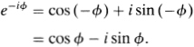
By adding and subtracting these formulas Euler obtained the following expressions for cos ϕ and sin ϕ:
![]()
These two formulas are the basis of modern analytic trigonometry.
The credit given to Euler for rediscovering Cotes’s formula is not entirely undeserved: whereas Cotes (as also his contemporary De Moivre) was still treating complex numbers merely as a convenient, if mysterious, way of shortening algebraic computations, it was Euler who fully incorporated these numbers into the algebra of functions. His idea was that a complex number can be used as an input to a function, provided the output is also a complex number.
Take, for example, the function w = sin z, where both z and w are complex variables. Writing z = x + iy, w = u + iv and proceeding as if the laws of ordinary trigonometry still hold, we get
![]()
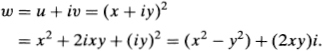
But what are cos iy and sin iy? Again proceeding in a purely formal way, let us substitute iy for ϕ in equations (2):
It so happens that the expressions (ey + e−y)/2 and (ey − e−y)/2 exhibit many formal similarities with the functions cos y and sin y, respectively, and are consequently denoted by cosh y and sinh y (read “hyperbolic cosine” and “hyperbolic sine” of y):
![]()
For example, if we square the two expressions and subtract the results, we get the identity
![]()
in analogy with the trigonometric identity cos2 y + sin2 y = 1 (note, however, the minus sign of the second term). We also have cosh 0 = 1, sinh 0 = 0, cosh (−y) = cosh y, sinh (−y) = −sinh y, cosh (x ± y) = cosh x cosh y ± sinh x sinh y, sinh (x ± y) = sinh x cosh y ± cosh x sinh y, and d (cosh y)/dy = sinh y, d (sinh y)/dy = cosh y. It turns out that most of the familiar trigonometric formulas have their hyperbolic counterparts, with a possible change of sign in one of the terms.3
We can now write equation (3) as
![]()
where again z = x + iy. In exactly the same way we can find an expression for cos z:
![]()
As an example, let us find the sine of the complex number z = 3 + 4i. Taking all units in radians, we have sin 3 = 0.141, cosh 4 = 27.308, cos 3 = −0.990 and sinh 4 = 27.290 (all rounded to three places), so sin z = sin 3 cosh 4 + i cos 3 sinh 4 = 3.854 − 27.017i.
There is, of course, one serious flaw in what we have just done: the very assumption that the familiar rules of algebra and trigonometry of real numbers still hold when applied to complex numbers. There is really no a priori guarantee that this should be the case; indeed, occasionally these rules break down when extended beyond their original domain: we may not, for example, use the rule √a · √b = √ab when a and b are negative, for otherwise we would have i2 = (√−1) · (√−l) = √[(−l) · (−1)] = √l = 1, instead of −1. But these subtleties did not prevent Euler from playing with his new idea: he lived in an era when a care-free manipulation of symbols was still accepted, and he made the most of it. He simply had faith in his formulas, and usually he was right. His daring and imaginative explorations resulted in numerous new relations whose rigorous proof had to await future generations.
Of course, an act of faith is not always a reliable guide in science, least of all in mathematics. The theory of functions of a complex variable, or theory of functions, as it is known for short, was created in part to put Euler’s ideas on a firm ground. It does this by essentially turning the tables around: we define a function w = f(z) in such a way that all the properties of the real-valued function y = f(x) will be preserved when x and y are replaced by the complex variables z and w. Moreover, we should always be able to get back the “old” function f(x) as a special case of the “new” function when z is a real variable x (that is, when z = x + 0i).
Let us illustrate these ideas with the sine and cosine functions. Using equations (6) and (7) as the definitions of sin z and cos z, we can show that sin2 z + cos2 z = 1, that each has a period 2π (that is, sin(z + 2π) = sin z for all z, and similarly for cos z), and that the familiar addition formulas still hold. Under certain conditions we can even differentiate a complex-valued function f(z), giving us (formally) the same derivative as we would get when differentiating the real-valued function y = f(x);4 in our case we have d(sinz)/dz = cos z and d(cosz)/dz = − sin z, exactly as in the real case.
But, you may ask, if the extension of a real-valued function to the complex domain merely reproduces its old properties, why go through the trouble? It would certainly not be worth the effort, were it not for the fact that this extension endows the function with some new properties unique to the complex domain. Foremost among these is the concept of a mapping from one plane to another.
To see this, we must first reexamine the function concept when applied to a complex variable. A real-valued function y = f(x) assigns to every real number x (the “input” or “independent variable”) in its domain one, and only one real number y (the “output” or “dependent variable”) in the range; it is thus a “mapping” from the x-axis to the y-axis. A convenient way to depict this mapping is to graph the function in the xy coordinate plane—in essence producing a pictorial representation that lets us see, quite literally, the manner in which the two variables depend on each other.
However, when we try to extend this idea to complex variables—that is, replace the real-valued function y = f(x) with the complex-valued function w = f(z)—we immediately encounter a difficulty. To plot a single complex number x + iy requires a two-dimensional coordinate system—one coordinate for the real part x and another for the imaginary part y. But now we are dealing with two complex variables, z and w, each of which requires its own two-dimensional coordinate system. We cannot therefore “graph” the function w = f(z) in the same sense as we graph the function y = f(x); to describe it geometrically, we need to think of it as a mapping from one plane to another.
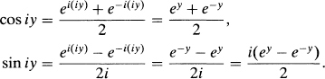
Let us illustrate this with the function w = z2, where z = x + iy and w = u + iv. We have
Equating real and imaginary parts, we get
![]()
Equations (8) tell us that both u and v are functions of the two independent variables x and y. Let us call the xy-plane the “z-plane” and the uv-plane the “w-plane.” Then the function w = z2 maps every point P(x, y) of the z-plane onto a corresponding point P′(u, v), the image of P in the w-plane; for example, the point P(3, 4) goes over to the point P′(−7, 24), as follows from the equation (3 + 4i)2 = −7 + 24i.
Imagine now that P describes some curve in the z-plane; then P′ will describe an “image curve” in the w-plane. For example, if P moves along the equilateral hyperbola x2 − y2 = constant, P′ will move along the curve u = constant, which is a vertical line in the w-plane. Similarly, if P traces the equilateral hyperbola 2xy = constant, its image will trace the horizontal line v = constant. By assigning different values to the constants, we get two families of hyperbolas in the z-plane; their images form a rectangular grid in the w-plane (fig. 88).
One of the most elegant results in the theory of functions says that the mapping effected by a function w = f(z) is conformal (direction-preserving) at all points z where it has a non-zero derivative.5 This means that if two curves in the z-plane intersect at a certain angle (the angle between their tangent lines at the point of intersection), their image curves in the w-plane will intersect at the same angle, provided df(z)/dz exists and is not zero at the point of intersection. This is clearly seen in the case of w = z2: the two families of hyperbolas, x2 − y2 = constant and 2xy = constant, are orthogonal—each hyperbola of one family intersects every hyperbola of the other at a right angle—as are their image curves, the horizontal and veritcal lines in the w-plane.
The mapping effected by the function w = sin z can be explored in a similar way. We start with horizontal lines y = c = constant in the z-plane. Equations (6) then tell us that
![]()
Equations (9) can be regarded as a pair of parametric equations describing a curve in the w-plane, the parameter being x. To get the rectangular equation of this curve, we must eliminate x between the two equations. We can do this by dividing the first equation by cosh c and the second by sinh c, squaring the results and adding; in view of the identity sin2x + cos2 x = 1 we get
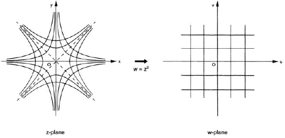
FIG. 88. Mapping by the function w = z2.
Equation (10) is of the form u2/a2 + v2/b2 = 1, which represents an ellipse with center at the origin of the w-plane, semimajor axis a = cosh c and semiminor axis b = |sinh c| (since cosh y is always greater than sinh y—as follows from equations 4—the major axis is always along the u-axis). Note that the ellipse will be traversed in a clockwise or counterclockwise sense, depending on whether c is positive or negative (this can best be seen from the parametric equations (9)). From analytic geometry we know that the two foci of the ellipse are located at the points (±f, 0), where f2 = a2 – b2. But a2 – b2 = cosh2 c − sinh2 c = 1, so we have f = ±1; for different values of c we therefore get a family of ellipses with a common pair of foci at (±1, 0), regardless of c. As c → 0, cosh c → 1 and sinh c → 0, so that the ellipses gradually narrow until they degenerate into the line segment − 1 ≤ u ≤ 1 along the u-axis. These features are shown in figure 89.
Next consider vertical lines x = k = constant in the z-plane. Equations (9) give us
![]()
This time we can eliminate the parameter y by dividing the first equation by sin k and the second by cos k, squaring the results and subtracting; in view of the identity cosh2 y − sinh2 y = 1 we get
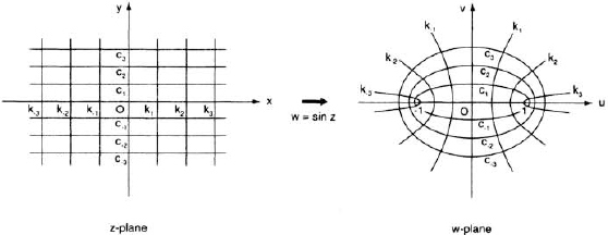
FIG. 89. Mapping by the function w = sin z.
Equation (12) is of the form u2/a2 − v2/b2 = 1, whose graph is a hyperbola with center at the origin, semi-transverse axis a = |sin K| and semi-conjugate axis b = |cos k| its asymptotes are the pair of lines y = ±[(cos k)/(sin k)]x = ±(cot k)x. As with the ellipses, it takes the pair of lines x = ±k to produce the entire hyperbola, the right branch corresponding to x = k (where k > 0), the left branch to x = −k. The two foci of the hyperbola are located at (±f, 0), where now f2 = a2 + b2 = sin2 k + cos2 k = 1; changing the value of k therefore produces a family of hyperbolas with a common pair of foci at (±1,0) (see fig. 89). As k → 0 the hyperbolas open up, and for k = 0 (corresponding to the x-axis in the z-plane) they degenerate into the line u = 0 (the v-axis in the w-plane). On the other hand, as |k| increases the hyperbolas narrow, degenerating into the pair of rays u ≥ 1 and u ≤ −1 when k = ±π/2. We also note that any increase of k by π does not change the values of sin2 k or cos2 k and so produces the same hyperbola; this, of course, merely shows that the mapping is not one-to-one, as we already know from the periodicity of sin z. Finally, the ellipses and hyperbolas form orthogonal families, as follows from the conformal property of complex-valued functions.6
![]()
As one more example we consider the function w = ez. First, of course, we must define what we mean by ez, so let us proceed formally by writing z = x + iy and acting as if the rules of algebra of real numbers are still valid:
ez = ex+iy = exeiy
But eiy = cos y + i sin y, so we have
![]()
We now regard equation (13) as the definition of ez. We note, first of all, that this is not a one-to-one function: increasing y by 2π does not change the value of ez, so we have ez + 2πi = ez. Consequently, the complex-valued exponential function has an imaginary period 2πi. This, of course, is in marked contrast to the real-valued function ex.
Writing w = ez = u + iv, equation (13) implies that
![]()
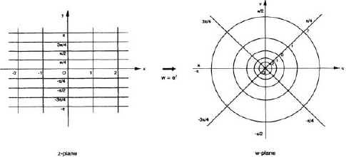
FIG. 90. Mapping by the function w = ez.
Putting y = c = constant in these equations and eliminating the parameter x, we get v = (tan c) u, the equation of a ray of slope tan c emanating from the origin of the w-plane; putting x = k = constant and eliminating y, we get u2 + v2 = e2k, representing a circle with center at the origin and radius ek. Thus the rectangular coordinate grid of the z-plane is mapped on a polar grid in the w-plane, with the circles spaced exponentially (fig. 90). Again the two grid systems are everywhere orthogonal.
We may discover here an unexpected connection with the map projections discussed in the previous chapter. To produce a polar grid in the w-plane with circles spaced linearly (rather than exponentially), we must increase k logarithmically; that is, vertical lines in the z-plane must be spaced as In k. The complex-valued function that accomplishes this is the inverse of w = ez, that is, w = In z. This mapping, when applied to the polar grid of a stereographic projection, gives us none other than Mercator’s grid—except that the roles of horizontal and vertical lines are reversed. But this reversal can be corrected by a 90° rotation of the coordinate system, that is, by a multiplication by i. We can therefore start with the globe, project it stereographically onto the z-plane, and then map this plane onto the w-plane by means of the function w = i ln z: the final product is Mercator’s projection. And since each of the component maps is conformal, so will be their product. As we recall, it was precisely this goal—to produce a conformal (direction-preserving) world map based on a rectangular grid—that led Mercator to his famous projection.
![]()
We began this chapter with the observation that no real angle exists whose sine is 2. But now that we have extended the functions sin x and cos x to the complex domain, let us try again. We wish to find an “angle” z = x + iy such that sin z = 2. From equations (6) it follows that
sin x cosh y = 2, cos x sinh y = 0.
The second of these equations implies that sinh y = 0 or cos x = 0; that is, y = 0 or x = (n + l/2)π, n = 0, ±1, ±2,…. Putting y = 0 in the first equation gives us (sin x)(cosh 0) = sin x = 2, which has no solution because x is a real number. Putting x = (n + l/2)π in the first equation gives us [sin (n + l/2)π](cosh y) = (−l)n cosh y = 2, so that cosh y = ±2. But the range of cosh y is [1, ∞), as follows from the defining equation cosh y = (ey + e−y)/2; hence we only need to consider cosh y = 2. Since cosh y is an even function, this equation has two equal but opposite solutions; these can be found from a table or a calculator that has hyperbolic-function capabilities: we find y = ±1.317, rounded to three places. Thus the equation sin z = 2 has infinitely many solutions z = (n + 1/2)π ± 1.317i, where n = 0, ±1, ±2,…. None of these solutions is a real number.
All of this may seem quite abstract and removed from ordinary trigonometry; it is certainly strange to talk of imaginary angles and their sines. Yet strangeness is a relative concept; with sufficient familiarity, the “strange” of yesterday becomes the commonplace of today. When negative numbers began to appear on the mathematical scene, they were at first regarded as strange, artificial creations (“how can one subtract five objects from four?”). A similar reaction awaited imaginary numbers, as attested by the very name “imaginary.” When Euler pioneered the extension of ordinary functions to the complex domain, his bold conclusions were strange and controversial; he was the first, for example, to define the logarithm of a negative number in terms of imaginary numbers—this at a time when even the existence of imaginary numbers was not yet entirely accepted.
It took the authority of Gauss to fully incorporate complex numbers into algebra; this he did in 1799 in his doctoral dissertation at the age of twenty-one, in which he gave the first rigorous demonstration of the fundamental theorem of algebra: a polynomial of degree n has exactly n (not necessarily different) roots in the complex number system.7 And any lingering doubts as to the “existence” of these numbers were put to rest when Sir William Rowan Hamilton (1805–1865) in 1835 presented his elegant definition of complex numbers as pairs of real numbers subject to a formal set of rules.8 The door was now open to a vast expansion of the methods of analysis to complex variables, culminating in the theory of functions with its numerous applications in nearly every branch of mathematics, pure or applied. The “strange” of yesterday indeed became the commonplace of today.
NOTES AND SOURCES
1. On the history of negative numbers, see David Eugene Smith, History of Mathematics (1925; rpt. New York: Dover, 1958), vol. 2, pp. 257-260; on the history of imaginary and complex numbers, see ibid., pp. 261–268.
2. More on Cotes’s life and work can be found in Stuart Hollingdale, Makers of Mathematics (Harmondsworth, U.K.: Penguin Books, 1989), pp. 245-252.
3. Note, however, that the hyperbolic functions are not periodic and that their ranges are 1 ≤ cosh y ≤ ∞ and −∞ ≤ sinn y ≤ ∞. The name “hyperbolic” comes from the fact that if we write x = cosh t, y = sinh t (where t is a real parameter), then the identity cosh2 t − sinh2 t = 1 implies that a point with coordinates (x, y) lies on the equilateral hyperbola x2 − y2 = 1, just as a point with coordinates x = cos t, y = sin t lies on the unit circle x2 + y2 = 1. For a history of the hyperbolic functions, see my book, e: The Story of a Number (Princeton, N.J.: Princeton University Press, 1994), pp. 140-150 and 208-210.
4. However, the concept of a derivative of a complex-valued function involves some subtleties that are not present in the real domain. An alternative approach, due to the German mathematician Karl Weierstrass (1815–1897), is to define a function by means of a power series, in the case of sin z the series z − z3/3! + z5/5 + – ···. For details, see any book on the theory of functions.
5. This is a far-reaching result which we have stated here only in brief form; for the complete theorem, see any book on the theory of functions.
6. For a more detailed discussion of the mapping w = sin z, see Erwing Kreiszig, Advanced Engineering Mathematics (New York: John Wiley, 1979), pp. 619-620.
7. For example, the polynomial f(z) = z3 − 1 has the three roots 1, (−1 − i√3)/2, and (−1 + √3)/2, as can be seen by factoring f(z) into (z − l)(z2 + z + 1), setting each factor equal to zero and solving the resulting equations. These “cubic roots of unity” can be written in trigonometric form as cis 0, cis 2π/3, and cis 4π/3, where “cis” stands for cos + i sin. It always surprises students to learn that the number 1 has three cubic roots, two of which are complex.
8. See Maor, e: The Story of a Number, pp. 166-168.